Research Article Analyzing Big Data with the Hybrid Interval Regression Methods

(1)

Research Article

Analyzing Big Data with the Hybrid Interval

Regression Methods

Chia-Hui Huang,

1

Keng-Chieh Yang,

2

and Han-Ying Kao

3

1_{Department of Business Administration, National Taipei University of Business, No. 321, Section 1, Jinan Road,} Zhongzheng District, Taipei City 100, Taiwan

2_{Department of Information Management, Hwa Hsia Institute of Technology, No. 111, Gongzhuan Road,} Zhonghe District, New Taipei City 235, Taiwan

3_{Department of Computer Science and Information Engineering, National Dong Hwa University,} No. 123, Hua-Shi Road, Hualien 97063, Taiwan

Correspondence should be addressed to Chia-Hui Huang; [email protected] Received 19 May 2014; Accepted 7 July 2014; Published 20 July 2014

Academic Editor: Jung-Fa Tsai

Copyright © 2014 Chia-Hui Huang et al. This is an open access article distributed under the Creative Commons Attribution License, which permits unrestricted use, distribution, and reproduction in any medium, provided the original work is properly cited.

Big data is a new trend at present, forcing the significant impacts on information technologies. In big data applications, one of the most concerned issues is dealing with large-scale data sets that often require computation resources provided by public cloud services. How to analyze big data efficiently becomes a big challenge. In this paper, we collaborate interval regression with the smooth support vector machine (SSVM) to analyze big data. Recently, the smooth support vector machine (SSVM) was proposed as an alternative of the standard SVM that has been proved more efficient than the traditional SVM in processing large-scale data. In addition the soft margin method is proposed to modify the excursion of separation margin and to be effective in the gray zone that the distribution of data becomes hard to be described and the separation margin between classes.

1. Introduction

Big data has become one of new research frontiers. Generally speaking, big data is a collection of large-scale and complex data sets that it becomes more difficult to process using current database management systems and traditional data processing applications. In 2012, Gartner Inc. gave a defini-tion of big data as “Big data is high volume, high velocity, and/or high variety information assets that require new forms of processing to enable enhanced decision making, insight

discovery and process optimization” [1]. The trend of big

data sets is due to the additional information derivable from analysis of a single large set of related data, as compared to separate smaller sets with the same total amount of data.

One of the major applications of the future parallel,

distributed, and cloud systems is in big data analytic [2–5].

Most concerned issues are dealing with large-scale sets which often require computation resources provided by public cloud

services. How to analyze big data efficiently becomes a big challenge.

The support vector machine (SVM) has shown to be an efficient approach for a variety of data mining, classification, analysis, pattern recognition, and distribution estimation

[6–14]. Recently, using SVM to solve the interval

regres-sion model [15] has become an alternative approach. Hong

and Hwang [16] evaluated interval regression models with

quadratic loss SVM. Bisserier et al. [17] proposed a revisited

fuzzy regression method where a linear model is identified from Crisp-Inputs Fuzzy-Outputs (CISO) data. D’Urso et al.

[18] presented fuzzy clusterwise regression analysis with LR

fuzzy response variable and numeric explanatory variables. The suggested model is to allow for linear and nonlinear relationship between the output and input variables. Jeng

et al. [19] developed a support vector interval regression

networks (SVIRNs) based on both SVM and neural networks.

Huang and Kao [20] proposed a soft-margin SVM for interval

Volume 2014, Article ID 243921, 8 pages http://dx.doi.org/10.1155/2014/243921

(2)

regression analysis. Huang [21] solved interval regression model with reduced support vector machine.

However, there are several main problems while using SVM model.

(1) Big data: when dealing with big data sets, the solution by using SVM with a nonlinear kernel may be difficult to be found.

(2) Noises and interaction: the distribution of data becomes hard to be described and the separation margin between classes becomes a “gray” zone. (3) Unbalance: the number of samples from one class is

much larger than the number of samples from other classes. It causes the excursion of separation margin. Under this circumstance, developing an efficient method to analyze big data becomes important. The smooth support vector machine (SSVM) has been proved more efficient than

the traditional SVM in processing large-scale data [22–24].

The main idea of SSVM is solved by a fast Newton-Armijo

algorithm [25] and has been extended to nonlinear separation

surfaces by using a nonlinear kernel technology [24].

In this study, we collaborate interval regression [15] with

SSVM to analyze big data. The main idea of SSVM is solved by a fast Newton-Armijo algorithm and has been extended to nonlinear separation surfaces by using a nonlinear kernel technology. Additionally, to modify the excursion of sepa-ration margin and to be effective in the gray zone, the soft margin method is proposed. The experiment results show that the proposed methods are more efficient than existing methods.

This study is organized as follows.Section 2reviews the

current methods for interval regression analysis.Section 3

proposes the soft margin method and the formulation of

interval regression with SSVM to analyze big data.Section 4

gives a numerical example by the proposed methods dealing with big data which is extracted from Taiwan Stock Exchange

Capitalization Weighted Stock Index (TAIEX) [26]. Finally,

Section 5gives the concluding remarks.

2. Literature Review

Since Tanaka et al. [27] introduced the fuzzy regression model

with symmetric fuzzy parameters, the properties of fuzzy regression have been studied extensively by many researchers. Fuzzy regression model can be simplified to interval regres-sion analysis which is considered as the simplest verregres-sion of possibilistic regression analysis with interval coefficients. An interval linear regression model is described as

𝑌 (x_𝑗) = 𝐴₀+ 𝐴₁𝑥_1𝑗+ ⋅ ⋅ ⋅ + 𝐴_𝑛𝑥_𝑛𝑗, (1)

where 𝑌(x_𝑗), 𝑗 = 1, 2, . . . , 𝑞, is the estimated interval

cor-responding to the real input vectorx_𝑗 = (𝑥_1𝑗, 𝑥_2𝑗, . . . , 𝑥_𝑛𝑗)𝑡.

An interval coefficient𝐴_𝑖is defined as(𝑎_𝑖, 𝑐_𝑖), where𝑎_𝑖is the

center and𝑐_𝑖is the radius. Hence,𝐴_𝑖can also be represented

as

𝐴_𝑖= [𝑎_𝑖− 𝑐_𝑖, 𝑎_𝑖+ 𝑐_𝑖] = {𝑎_𝑖− 𝑐_𝑖≤ 𝑎 ≤ 𝑎_𝑖+ 𝑐_𝑖} . (2)

The interval linear regression model (1) can also be

expressed as 𝑌 (x_𝑗) = 𝐴₀+ 𝐴₁𝑥_1𝑗+ ⋅ ⋅ ⋅ + 𝐴_𝑛𝑥_𝑛𝑗 = (𝑎₀, 𝑐₀) + (𝑎₁, 𝑐₁) 𝑥_1𝑗+ ⋅ ⋅ ⋅ + (𝑎_𝑛, 𝑐_𝑛) 𝑥_𝑛𝑗 = (𝑎₀+∑𝑛 𝑖=1 𝑎_𝑖𝑥_𝑖𝑗, 𝑐₀+∑𝑛 𝑖=1 𝑐_𝑖󵄨󵄨󵄨󵄨_󵄨𝑥𝑖𝑗󵄨󵄨󵄨󵄨_{󵄨) .} (3)

For a data set with crisp inputs and interval outputs, two interval regression models, the possibility and necessity mod-els, are considered. By assumption, the center coefficients of the possibility regression model and the necessity regression

model are the same [15]. For this data set, the possibility and

necessity estimation models are defined as

𝑌∗(x_𝑗) = 𝐴∗₀+ 𝐴∗₁𝑥_1𝑗+ ⋅ ⋅ ⋅ + 𝐴∗_𝑛𝑥_𝑛𝑗

𝑌_∗(x_𝑗) = 𝐴_0∗+ 𝐴_1∗𝑥_1𝑗+ ⋅ ⋅ ⋅ + 𝐴_𝑛∗𝑥_𝑛𝑗, (4)

where the interval coefficients𝐴∗_𝑖and𝐴_𝑖∗are defined as𝐴∗_𝑖 =

(𝑎∗

𝑖, 𝑐𝑖∗)and𝐴𝑖∗= (𝑎𝑖∗, 𝑐𝑖∗), respectively. The interval𝑌∗(x𝑗)

estimated by the possibility model must include the observed

interval𝑌_𝑗and the interval𝑌_∗(x_𝑗)estimated by the necessity

model must be included in the observed interval𝑌_𝑗.

In this section, we review the current methods which are ordinarily used for interval regression analysis.

2.1. Tanaka and Lee’s Approach. Tanaka and Lee [15] posed an interval regression analysis with a quadratic pro-gramming (QP) approach which gives more diverse spread coefficients than a linear programming (LP) one.

The interval regression analysis by QP approach unifying the possibility and necessity models subject to the inclusion

relations,𝑌_∗(x_𝑗) ⊆ 𝑌_𝑗 ⊆ 𝑌∗(x_𝑗), can be represented as

min 𝑞 ∑ 𝑗=1 (𝑑₀+∑𝑛 𝑖=1 𝑑_𝑖󵄨󵄨󵄨󵄨_󵄨𝑥𝑖𝑗󵄨󵄨󵄨󵄨_󵄨) 2 + 𝜑∑𝑛 𝑖=0 (𝑎_𝑖2+ 𝑐_𝑖2) s.t. 𝑌_∗(x_𝑗) ⊆ 𝑌_𝑗 ⊆ 𝑌∗(x_𝑗) , 𝑗 = 1, 2, . . . , 𝑞 𝑐_𝑖, 𝑑_𝑖≥ 0, 𝑖 = 0, 1, . . . , 𝑛, (5)

where𝜑is an extremely small positive number and makes

(3)

function negligible. The constraints of the inclusion relations are equivalent to 𝑌_∗(x_𝑗) ⊆ 𝑌_𝑗⇐⇒ { { { { { { { { { { { 𝑦_𝑗− 𝑒_𝑗 ≤ (𝑎₀+∑𝑛 𝑖=1 𝑎_𝑖𝑥_𝑖𝑗) − (𝑐₀+∑𝑛 𝑖=1 𝑐_𝑖󵄨󵄨󵄨󵄨_󵄨𝑥𝑖𝑗󵄨󵄨󵄨󵄨_󵄨) (𝑎₀+∑𝑛 𝑖=1 𝑎_𝑖𝑥_𝑖𝑗) + (𝑐₀+∑𝑛 𝑖=1 𝑐_𝑖󵄨󵄨󵄨󵄨_󵄨𝑥𝑖𝑗󵄨󵄨󵄨󵄨_{󵄨) ≤ 𝑦}_𝑗+ 𝑒_𝑗, (6) 𝑌_𝑗⊆ 𝑌∗(x_𝑗) ⇐⇒ { { { { { { { { { { { { { { { { { { { { { { { { { { { { { (𝑎₀+∑𝑛 𝑖=1 𝑎_𝑖𝑥_𝑖𝑗) − (𝑐₀+∑𝑛 𝑖=1 𝑐_𝑖󵄨󵄨󵄨󵄨_󵄨𝑥𝑖𝑗󵄨󵄨󵄨󵄨_󵄨) − (𝑑₀+∑𝑛 𝑖=1 𝑑_𝑖󵄨󵄨󵄨󵄨_󵄨𝑥𝑖𝑗󵄨󵄨󵄨󵄨_{󵄨) ≤ 𝑦}_𝑗− 𝑒_𝑗 𝑦_𝑗+ 𝑒_𝑗 ≤ (𝑎₀+∑𝑛 𝑖=1 𝑎_𝑖𝑥_𝑖𝑗) + (𝑐₀+∑𝑛 𝑖=1 𝑐_𝑖󵄨󵄨󵄨󵄨_󵄨𝑥𝑖𝑗󵄨󵄨󵄨󵄨_󵄨) + (𝑑0+ 𝑛 ∑ 𝑖=1𝑑𝑖󵄨󵄨󵄨󵄨󵄨𝑥𝑖𝑗󵄨󵄨󵄨󵄨󵄨) , (7)

wherex_𝑗 is the𝑗th input vector and𝑌_𝑗 is the corresponding

interval output that consists of a center𝑦_𝑗 and a radius𝑒_𝑗

denoted by𝑌_𝑗= (𝑦_𝑗, 𝑒_𝑗).

2.2. Hong and Hwang’s Approach. Hong and Hwang [16] evaluated interval regression model combining the possibility and necessity estimation formulation with the principle of quadratic loss support vector machine (QLSVM). This version of SVM utilizes the quadratic loss function. The QLSVM performs interval nonlinear regression analysis by constructing an interval linear regression function in high-dimensional feature space.

With the principle of QLSVM, the interval nonlinear regression model is given as follows:

max −1 2( 𝑛 ∑ 𝑖,𝑗=1 (𝜆_2𝑖− 𝜆∗_2𝑖) (𝜆_2𝑗− 𝜆∗_2𝑗) 𝐾 (x_𝑖,x_𝑗) + ∑𝑛 𝑖,𝑗=1 (𝜆3𝑖− 𝜆∗3𝑖) (𝜆3𝑗− 𝜆∗3𝑗) 𝐾 (x𝑖,x𝑗) + ∑𝑛 𝑖,𝑗=1 (𝜆_4𝑖− 𝜆∗_4𝑖) (𝜆_4𝑗− 𝜆∗_4𝑗) 𝐾 (x_𝑖,x_𝑗) + 2∑𝑛 𝑖,𝑗=1 (𝜆_2𝑖− 𝜆∗_2𝑖) (𝜆_3𝑗− 𝜆∗_3𝑗) 𝐾 (x_𝑖,x_𝑗) − 2∑𝑛 𝑖,𝑗=1 (𝜆_2𝑖− 𝜆∗_2𝑖) (𝜆_4𝑗− 𝜆∗_4𝑗) 𝐾 (x_𝑖,x_𝑗) − 2∑𝑛 𝑖,𝑗=1(𝜆3𝑖− 𝜆 ∗ 3𝑖) (𝜆4𝑗− 𝜆∗4𝑗) 𝐾 (x𝑖,x𝑗) + ∑𝑛 𝑖,𝑗=1 (𝜆_3𝑖+ 𝜆∗_3𝑖) (𝜆_3𝑗+ 𝜆_3𝑗∗_{) 𝐾 (󵄨󵄨󵄨󵄨}x_𝑖󵄨󵄨󵄨󵄨,󵄨󵄨󵄨󵄨󵄨x_𝑗󵄨󵄨󵄨󵄨_󵄨) + ∑𝑛 𝑖,𝑗=1 (𝜆_4𝑖+ 𝜆∗_4𝑖) (𝜆_4𝑗+ 𝜆∗_{4𝑗) 𝐾 (󵄨󵄨󵄨󵄨}x_𝑖󵄨󵄨󵄨󵄨,󵄨󵄨󵄨󵄨󵄨x_𝑗󵄨󵄨󵄨󵄨_󵄨) − 2∑𝑛 𝑖,𝑗=1 (𝜆_3𝑖+ 𝜆∗_3𝑖) (𝜆_4𝑗+ 𝜆∗_{4𝑗) 𝐾 (󵄨󵄨󵄨󵄨}x_𝑖󵄨󵄨󵄨󵄨,󵄨󵄨󵄨󵄨󵄨x𝑗󵄨󵄨󵄨󵄨_󵄨) + ∑𝑛 𝑖,𝑗=1 𝜆_1𝑖𝜆_1𝑗_{𝐾 (󵄨󵄨󵄨󵄨}x_𝑖󵄨󵄨󵄨󵄨,󵄨󵄨󵄨󵄨󵄨x_𝑗󵄨󵄨󵄨󵄨_󵄨) − 2∑𝑛 𝑖,𝑗=1𝜆1𝑖(𝜆3𝑗+ 𝜆 ∗ 3𝑗) 𝐾 (󵄨󵄨󵄨󵄨x𝑖󵄨󵄨󵄨󵄨,󵄨󵄨󵄨󵄨󵄨x𝑗󵄨󵄨󵄨󵄨_󵄨)) − 1 2𝐶 𝑛 ∑ 𝑖=1 𝜆2_1𝑖− 1 2𝐶 𝑛 ∑ 𝑖=1 (𝜆2_2𝑖+ 𝜆∗2_2𝑖) +∑𝑛 𝑖=1 (𝜆_2𝑖− 𝜆∗ 2𝑖) 𝑦𝑖+ 𝑛 ∑ 𝑖=1 (𝜆_3𝑖− 𝜆∗ 3𝑖) 𝑦𝑖 −∑𝑛 𝑖=1(𝜆4𝑖− 𝜆 ∗ 4𝑖) 𝑦𝑖 +∑𝑛 𝑖=1 (𝜆_3𝑖+ 𝜆∗_3𝑖) 𝜖_𝑖−∑𝑛 𝑖=1 (𝜆_4𝑖+ 𝜆∗_4𝑖) 𝜖_𝑖 s.t. 𝜆_1𝑖, 𝜆_2𝑖, 𝜆∗_2𝑖, 𝜆_3𝑖, 𝜆∗_3𝑖, 𝜆_4𝑖, 𝜆∗_4𝑖≥ 0, (8)

where 𝜆_1𝑖, 𝜆_2𝑖, 𝜆∗_2𝑖, 𝜆_3𝑖, 𝜆∗_3𝑖, 𝜆_4𝑖, and 𝜆∗_4𝑖 are Lagrange

multipliers. 𝐾(∗) is a nonlinear kernel. The followings are

well-known nonlinear kernels, where𝜎, 𝛾, 𝑟, ℎ, and𝜃 are

kernel parameters:

(1) Gaussian (radial basis) kernel:𝑒−‖𝑥𝑖−𝑥𝑗‖2/2𝜎2_, 𝜎 > 0

[10],

(2) hyperbolic tangent kernel: tanh(𝛾𝑥_𝑖𝑥𝑡_𝑗+𝜃),𝛾 > 0[12],

(3) polynomial kernel:(𝛾𝑥_𝑖𝑥𝑡_𝑗+ 𝑟)ℎ,ℎ ∈ N,𝛾 > 0, and

𝑟 ≥ 0[14].

The advantage of Hong and Hwang’s approach is a model-free method in the sense that there is no need to assume the underlying model function for interval nonlinear regression model with crisp inputs and interval output.

2.3. Huang’s Approach. There are two problems while using the traditional SVM model. (1) Large scale: when dealing with large-scale data sets, the solution may be difficult to be found when using SVM with nonlinear kernels; (2) Unbalance: the number of samples from one class is much larger than the number of samples from the other classes. It causes the excursion of separation margin.

To resolve these problems, Huang [21] proposed a

reduced support vector machine (RSVM) approach in eval-uating interval regression models. RSVM has been proven

(4)

more efficient than the traditional SVM in processing large-scale data.

With the principle of RSVM, the interval nonlinear regression model is listed as follows:

max −1 2 𝑛 ∑ 𝑖,𝑗=1 𝜆_1𝑖𝜆_1𝑗𝑄𝑡_⋅,𝐾𝑄_⋅,𝐾 −1₂∑𝑛 𝑖,𝑗=1 (𝜆_2𝑖− 𝜆∗_2𝑖) (𝜆_2𝑗− 𝜆∗_2𝑗) 𝐾 (x_𝑖,x_𝑗) −1 2 𝑛 ∑ 𝑖,𝑗=1 (𝜆_3𝑖− 𝜆∗_3𝑖) (𝜆_3𝑗− 𝜆∗_3𝑗) 𝐾 (x_𝑖,x_𝑗) − ∑𝑛 𝑖,𝑗=1 𝜆_1𝑖𝑄_⋅,𝐾(𝜆_2𝑗− 𝜆∗_2𝑗)x_𝑗 + ∑𝑛 𝑖,𝑗=1 𝜆_1𝑖𝑄_⋅,𝐾(𝜆_3𝑗− 𝜆∗_3𝑗)x_𝑗 + ∑𝑛 𝑖,𝑗=1(𝜆2𝑖− 𝜆 ∗ 2𝑖) (𝜆3𝑗− 𝜆∗3𝑗) 𝐾 (x𝑖,x𝑗) −1 2 𝑛 ∑ 𝑖,𝑗=1 (𝜆_2𝑖+ 𝜆∗_2𝑖) (𝜆_2𝑗+ 𝜆∗_{2𝑗) 𝐾 (󵄨󵄨󵄨󵄨}x_𝑖󵄨󵄨󵄨󵄨,󵄨󵄨󵄨󵄨󵄨x𝑗󵄨󵄨󵄨󵄨_󵄨) + ∑𝑛 𝑖,𝑗=1 (𝜆_2𝑖+ 𝜆∗_2𝑖) (𝜆_3𝑗+ 𝜆∗_{3𝑗) 𝐾 (󵄨󵄨󵄨󵄨}x_𝑖󵄨󵄨󵄨󵄨,󵄨󵄨󵄨󵄨󵄨x_𝑗󵄨󵄨󵄨󵄨_󵄨) − ∑𝑛 𝑖,𝑗=1 (𝜆_3𝑖+ 𝜆∗_3𝑖) (𝜆_3𝑗+ 𝜆∗_3𝑗_{) 𝐾 (󵄨󵄨󵄨󵄨}x_𝑖󵄨󵄨󵄨󵄨,󵄨󵄨󵄨󵄨󵄨x_𝑗󵄨󵄨󵄨󵄨_󵄨) − 1 4𝐶 𝑛 ∑ 𝑖=1 𝜆2 1𝑖+ 𝑛 ∑ 𝑖=1 (𝜆_2𝑖− 𝜆∗ 2𝑖) 𝑦𝑖 −∑𝑛 𝑖=1 (𝜆3𝑖− 𝜆∗3𝑖) 𝑦𝑖 −∑𝑛 𝑖=1 (𝜆_2𝑖+ 𝜆∗_2𝑖) 𝜖_𝑖+∑𝑛 𝑖=1 (𝜆_3𝑖+ 𝜆∗_3𝑖) 𝜖_𝑖 s.t. 𝜆_1𝑖, 𝜆_2𝑖, 𝜆∗_2𝑖, 𝜆_3𝑖, 𝜆∗_3𝑖≥ 0, (9)

where𝜆_1𝑖,𝜆_2𝑖,𝜆∗_2𝑖,𝜆_3𝑖, and𝜆∗_3𝑖are Lagrange multipliers.𝑄is

a positive semidefinite matrix in RSVM.𝐾(∗)is a nonlinear

kernel.

The advantage of Huang’s approach is to reduce the number of support vectors by randomly selecting a subset of samples. While processing with large-scale data sets, the solution can be found easily by the proposed method with nonlinear kernels.

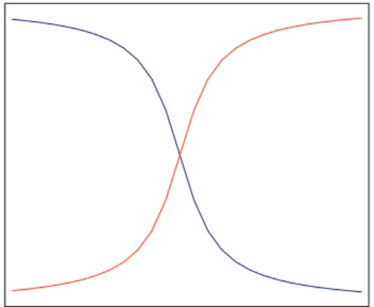
Figure 1: Soft margin.

3. Proposed Methods

In this section we first propose the soft margin method to modify the excursion of separation margin and to be effective in the gray zone. Then the formulation of interval regression with SSVM to analyze big data is introduced.

3.1. Soft Margin. In a conventional SVM, the sign function is used as the decision-making function. The separation thresh-old of the sign function is 0, which results in an excursion of separation margin for unbalanced data sets. The aim of the hard-margin separation margin is to find a hyperplane with the largest distance to the nearest training data. However, the limitations of the hard-margin formulation are as follows:

(1) there is no separating hyperplane for certain training data;

(2) complete separation with zero training error will lead to suboptimal prediction error;

(3) it is difficult to deal with the gray zone between classes.

Thus, the soft margin method is proposed to modify the excursion of separation margin and to be effective in the gray zone. The soft margin is defined as

𝑓−(𝛿) = arctan(−𝛿 ⋅ 𝑠 + 𝜗 ⋅ 𝑠)

𝜋 + 0.5,

𝑓+(𝛿) = arctan(𝛿 ⋅ 𝑠 − 𝜗 ⋅ 𝑠)_𝜋 + 0.5,

(10)

where𝛿is the decision value.𝜗and𝑠are offset parameter and

scale parameter which need to be estimated using statistical method.

With the soft margin as shown inFigure 1, the predication

of the class labels can be determined as follows:

𝑦 (𝑥)

= {−1,_+1, if (]𝑟 < 𝑓−(𝛿) , 𝛿 < 𝜗) or (]𝑟 > 𝑓+(𝛿) , 𝛿 > 𝜗)

if (]_𝑟 > 𝑓−(𝛿) , 𝛿 < 𝜗) or (]_𝑟 < 𝑓+(𝛿) , 𝛿 > 𝜗) , (11)

(5)

3.2. Interval Regression with SSVM. The main idea of smooth support vector machine (SSVM) is solved by a fast

Newton-Armijo algorithm [25] and has been extended to nonlinear

separation surfaces by using a nonlinear kernel technology

[24].

Suppose that𝑚training data{𝑥_𝑖, 𝑦_𝑖},𝑖 = 1, 2, . . . , 𝑚, are

given, where𝑥_𝑖∈R𝑛are the input patterns and𝑦_𝑖 ∈ {−1, 1}

are the related target values of two-class pattern classification case. Then the standard support vector machine with a linear

kernel [14] is min 𝑤,𝑏,𝜉 1 2‖𝑤‖2+ 𝐶 𝑚 ∑ 𝑖=1 𝜉_𝑖2 s.t. 𝑦_𝑖(𝑤𝑡𝑥_𝑖+ 𝑏) ≥ 1 − 𝜉_𝑖 𝜉_𝑖≥ 0, 𝑖 = 1, 2, . . . , 𝑚, (12)

where𝑏is the location of hyperplane relative to the origin.

The regularization constant 𝐶 is a positive parameter to

control the tradeoff between the training error and the part of

maximizing the margin that is achieved by minimizing‖𝑤‖2.

𝜉_𝑖is the slack variable with weight𝐶/2.‖𝑤‖is the Euclidean

norm of𝑤which is the normal to the following hyperplanes:

𝑤𝑡𝑥_𝑖+ 𝑏 = +1, for𝑦_𝑖= +1, (13)

𝑤𝑡𝑥_𝑖+ 𝑏 = −1, for𝑦_𝑖= −1. (14)

The first hyperplane (13) bounds the class{+1}and the

second hyperplane (14) bounds the class {−1}. The linear

separating hyperplane is

𝑤𝑡𝑥_𝑖+ 𝑏 = 0. (15)

In Lee and Mangasarian’s approach [24],𝑏2/2is added to

the objective function of (12). This is equivalent to adding a

constant feature to the training data and finding a separating hyperplane through the origin. Consider

min 𝑤,𝑏,𝜉 1 2(‖𝑤‖2+ 𝑏2) + 𝐶 2 𝑚 ∑ 𝑖=1 𝜉2 𝑖 s.t. 𝑦_𝑖(𝑤𝑡𝑥_𝑖+ 𝑏) ≥ 1 − 𝜉_𝑖 𝜉𝑖≥ 0, 𝑖 = 1, 2, . . . , 𝑚, (16)

where𝜉_𝑖 = {1 − 𝑦_𝑖(𝑤𝑡𝑥_𝑖+ 𝑏)}₊ for all𝑖and the “+” function

is defined as𝑥₊ =max{0, 𝑥}. Then (12) can be reformulated

as the following minimization problem by replacing𝜉_𝑖with

{1 − 𝑦_𝑖(𝑤𝑡𝑥_𝑖+ 𝑏)}₊: min 𝑤,𝑏 1 2(‖𝑤‖2+ 𝑏2) + 𝐶 2 𝑚 ∑ 𝑖=1 {1 − 𝑦_𝑖(𝑤𝑡𝑥_𝑖+ 𝑏)}2₊. (17)

The objective function in (17) is not twice differentiable

and can be solved by using a fast Newton-Armijo method

[25]. Thus the “+” function in SSVM is approximated by a

smooth function,𝑝(𝑥, 𝛼), as follows:

𝑝 (𝑥, 𝛼) = 𝑥 +_𝛼1log(1 + 𝑒−𝛼𝑥) , 𝛼 > 0, (18)

where𝛼 > 0 is the smooth parameter.1/(1 + 𝑒−𝛼𝑥) is the

integral of the sigmoid function of neural networks [28].

The𝑝(𝑥, 𝛼)with a smoothing parameter𝛼 is to replace the

“+” function of (17) to obtain the following smooth support

vector machine (SSVM) with a linear kernel:

min 𝑤,𝑏 1 2(‖𝑤‖2+ 𝑏2) + 𝐶 2 𝑚 ∑ 𝑖=1 𝑝({1 − 𝑦_𝑖(𝑤𝑡_𝑥 𝑖+ 𝑏)} , 𝛼)2. (19)

For specific data sets, an appropriate nonlinear mapping

𝑥 󳨃→ 𝜙(𝑥)can be used to embed the originalR𝑛features into

a Hilbert feature spaceF,𝜙 : R𝑛 󳨃→ F, with a nonlinear

kernel𝐾(𝑥_𝑖, 𝑥_𝑗) ≡ 𝜙(𝑥_𝑖)𝑡𝜙(𝑥_𝑗). Thus, (19) can be extended to

the SSVM with a nonlinear kernel:

min 𝑤,𝑏 1 2(‖𝑤‖2+ 𝑏2) +𝐶 2 𝑚 ∑ 𝑖=1 𝑝({_{ { 1 − 𝑦_𝑖(∑𝑚 𝑗=1 V_𝑗𝐾 (𝑥_𝑖, 𝑥_𝑗) + 𝑏)}_} } , 𝛼) 2 , (20)

where∑𝑚_𝑗=1V_𝑗𝐾(𝑥_𝑖, 𝑥_𝑗) + 𝑏is the nonlinear SSVM classifier.

The coefficient V_𝑗 is determined by solving an

optimiza-tion problem (20) and the data points with corresponding

nonzero coefficients.

With the principle of SSVM, we can formulate the interval linear regression model as follows:

min 𝑎,𝑐,𝑑 1 2(𝑎𝑡𝑎 + 𝑐𝑡𝑐 + 𝑑 𝑡 𝑑 + 𝑏2) +𝐶₂∑𝑚 𝑖=1 𝑝({1 − 𝑦𝑖(𝑤𝑡𝑥𝑖+ 𝑏)} , 𝛼)2 s.t. 𝑎x_𝑖+ 𝑐 󵄨󵄨󵄨󵄨x_𝑖󵄨󵄨󵄨󵄨 ≤ 𝑦_𝑖+ 𝑒_𝑖 𝑎x_𝑖_{− 𝑐 󵄨󵄨󵄨󵄨}x_𝑖󵄨󵄨󵄨󵄨 ≥ 𝑦_𝑖− 𝑒_𝑖 𝑎x_𝑖_{+ 𝑐 󵄨󵄨󵄨󵄨}x_𝑖󵄨󵄨󵄨󵄨 + 𝑑󵄨󵄨󵄨󵄨x_𝑖󵄨󵄨󵄨󵄨 ≥ 𝑦_𝑖+ 𝑒_𝑖 𝑎x_𝑖_{− 𝑐 󵄨󵄨󵄨󵄨}x_𝑖󵄨󵄨󵄨󵄨 − 𝑑󵄨󵄨󵄨󵄨x_𝑖󵄨󵄨󵄨󵄨 ≤ 𝑦_𝑖− 𝑒_𝑖 𝑖 = 1, 2, . . . , 𝑚, (21)

where𝑎,𝑐, and𝑑are the collections of all𝑎_𝑖,𝑐_𝑖, and𝑑_𝑖,𝑖 =

(6)

Given (21), the corresponding Lagrangian objective func-tion is 𝐿 := 1 2(𝑎𝑡𝑎 + 𝑐𝑡𝑐 + 𝑑 𝑡 𝑑 + 𝑏2) +𝐶 2 𝑚 ∑ 𝑖=1 𝑝({1 − 𝑦_𝑖(𝑤𝑡𝑥_𝑖+ 𝑏)} , 𝛼)2 −∑𝑚 𝑖=1 𝜆_1𝑖(𝑦_𝑖+ 𝑒_𝑖− 𝑎x_𝑖_{− 𝑐 󵄨󵄨󵄨󵄨}x_𝑖󵄨󵄨󵄨󵄨) −∑𝑚 𝑖=1 𝜆2𝑖(𝑎x𝑖− 𝑐 󵄨󵄨󵄨󵄨x𝑖󵄨󵄨󵄨󵄨 − 𝑦𝑖+ 𝑒𝑖) −∑𝑚 𝑖=1 𝜆_3𝑖(𝑎x_𝑖_{+ 𝑐 󵄨󵄨󵄨󵄨}x_𝑖󵄨󵄨󵄨󵄨 + 𝑑󵄨󵄨󵄨󵄨x_𝑖󵄨󵄨󵄨󵄨 − 𝑦_𝑖− 𝑒_𝑖) −∑𝑚 𝑖=1 𝜆_4𝑖(𝑦_𝑖− 𝑒_𝑖− 𝑎x_𝑖_{+ 𝑐 󵄨󵄨󵄨󵄨}x_𝑖󵄨󵄨󵄨󵄨 + 𝑑󵄨󵄨󵄨󵄨x_𝑖󵄨󵄨󵄨󵄨), (22)

where𝐿is Lagrangian and𝜆_1𝑖,𝜆_2𝑖,𝜆_3𝑖, and𝜆_4𝑖are Lagrange

multipliers. The idea to construct a Lagrange function from the objective function and the corresponding constraints is to introduce a dual set of variables. It can be shown that the Lagrangian function has a saddle point with respect to the

primal and dual variables in the solution [29].

The Karush-Kuhn-Tucker (KKT) conditions that the

partial derivatives of𝐿with respect to the primal variables

(𝑎, 𝑐, 𝑑)for optimality 𝜕𝐿 𝜕𝑎 = 0 󳨐⇒ 𝑎 = − 𝑚 ∑ 𝑖=1 (𝜆_1𝑖− 𝜆_2𝑖− 𝜆_3𝑖+ 𝜆_4𝑖)x_𝑖, 𝜕𝐿 𝜕𝑐 = 0 󳨐⇒ 𝑐 = − 𝑚 ∑ 𝑖=1 (𝜆_1𝑖+ 𝜆_2𝑖− 𝜆_3𝑖− 𝜆_4𝑖_{) 󵄨󵄨󵄨󵄨}x_𝑖󵄨󵄨󵄨󵄨, 𝜕𝐿 𝜕𝑑 = 0 󳨐⇒ 𝑑 = 𝑚 ∑ 𝑖=1 (𝜆3𝑖+ 𝜆4𝑖) 󵄨󵄨󵄨󵄨x𝑖󵄨󵄨󵄨󵄨. (23)

Substituting (23) in (22) yields the following optimization

problem: max 1 2( 𝑚 ∑ 𝑖,𝑗=1 (𝜆_1𝑖− 𝜆_2𝑖− 𝜆_3𝑖+ 𝜆_4𝑖) × (𝜆1𝑗− 𝜆2𝑗− 𝜆3𝑗+ 𝜆4𝑗)x𝑡𝑖x𝑗 + ∑𝑚 𝑖,𝑗=1 (𝜆_1𝑖+ 𝜆_2𝑖− 𝜆_3𝑖− 𝜆_4𝑖) × (𝜆_1𝑗+ 𝜆_2𝑗− 𝜆_3𝑗− 𝜆_4𝑗_{) 󵄨󵄨󵄨󵄨}x_𝑖󵄨󵄨󵄨󵄨𝑡󵄨󵄨󵄨󵄨_󵄨x𝑗󵄨󵄨󵄨󵄨_󵄨 − ∑𝑚 𝑖,𝑗=1(𝜆3𝑖+ 𝜆4𝑖) (𝜆3𝑗+ 𝜆4𝑗) 󵄨󵄨󵄨󵄨x𝑖󵄨󵄨󵄨󵄨 𝑡󵄨󵄨󵄨󵄨 󵄨x𝑗󵄨󵄨󵄨󵄨_{󵄨 + 𝑏}2) +𝐶 2 𝑚 ∑ 𝑖=1 𝑝({1 − 𝑦_𝑖(𝑤𝑡𝑥_𝑖+ 𝑏)} , 𝛼)2 s.t. 𝜆_1𝑖, 𝜆_2𝑖, 𝜆_3𝑖, 𝜆_4𝑖≥ 0. (24) Similarly, we can obtain the interval nonlinear regression

model by mapping 𝑥 󳨃→ 𝜙(𝑥) to embed the original R𝑛

features into a Hilbert feature space F, 𝜙 : R𝑛 󳨃→ F,

with a nonlinear kernel𝐾(𝑥_𝑖, 𝑥_𝑗) ≡ 𝜙(𝑥_𝑖)𝑡𝜙(𝑥_𝑗)as discussed

inSection 2.2. Then we obtain the optimization problem as

(25) by replacingx𝑡_𝑖x_𝑗 and|x_𝑖|𝑡|x_𝑗|in (24) with𝐾(x_𝑖,x_𝑗)and

𝐾(|x_𝑖|, |x_𝑗|), respectively: max 1 2( 𝑚 ∑ 𝑖,𝑗=1 (𝜆_1𝑖− 𝜆_2𝑖− 𝜆_3𝑖+ 𝜆_4𝑖) × (𝜆_1𝑗− 𝜆_2𝑗− 𝜆_3𝑗+ 𝜆_4𝑗) 𝐾 (x_𝑖,x_𝑗) + ∑𝑚 𝑖,𝑗=1 (𝜆_1𝑖+ 𝜆_2𝑖− 𝜆_3𝑖− 𝜆_4𝑖) × (𝜆_1𝑗+ 𝜆_2𝑗− 𝜆_3𝑗− 𝜆_4𝑗_{) 𝐾 (󵄨󵄨󵄨󵄨}x_𝑖󵄨󵄨󵄨󵄨,󵄨󵄨󵄨󵄨󵄨x_𝑗󵄨󵄨󵄨󵄨_󵄨) − ∑𝑚 𝑖,𝑗=1 (𝜆_3𝑖+ 𝜆_4𝑖) × (𝜆_3𝑗+ 𝜆_4𝑗_{) 𝐾 (󵄨󵄨󵄨󵄨}x_𝑖󵄨󵄨󵄨󵄨,󵄨󵄨󵄨󵄨󵄨x_𝑗󵄨󵄨󵄨󵄨_{󵄨) + 𝑏}2) +𝐶₂∑𝑚 𝑖=1 𝑝({_{ { 1 − 𝑦_𝑖(∑𝑚 𝑗=1 V_𝑗𝐾 (x_𝑖,x_𝑗) + 𝑏)}_} } , 𝛼) 2 s.t. 𝜆_1𝑖, 𝜆_2𝑖, 𝜆_3𝑖, 𝜆_4𝑖≥ 0. (25)

4. Numerical Example

To illustrate the methods developed inSection 3, the

follow-ing example is presented.

Example. To illustrate the proposed methods dealing with big data sets, we use the data sets from Taiwan Stock

Exchange Capitalization Weighted Stock Index (TAIEX) [26]

which included the highest, lowest, and closed data and the

ranges are from01/02/2012to12/28/2012, from01/02/2011

to12/28/2012, from01/02/2010to 12/28/2012, and from

01/02/2009to12/28/2012, respectively. For these data sets,

the Gaussian kernel [10] is used where 𝜎 = 2.5 and the

regularization constant𝐶 = 300. The results are illustrated

fromFigure 2toFigure 5.

The comparison is shown by using the measure of fitness

(7)

Table 1: Comparison results of the measure of fitness.

Tanaka and Lee [15] Hong and Hwang [16] Huang [21] Proposed methods

𝜑_𝑌(Figure 2) 0.1404 0.1395 0.1412 0.1354 𝜑𝑌(Figure 3) 0.1573 0.1562 0.1581 0.1429 𝜑𝑌(Figure 4) 0.1694 0.1658 0.1706 0.1583 𝜑_𝑌(Figure 5) 0.1714 0.1695 0.1723 0.1609 TWSE TAIEX (01/02/2012~12/28/2012) 6.500.00 7.000.00 7.500.00 8.000.00 8.500.00 Highest Lowest TAIEX

Figure 2: TAIEX [26] from01/02/2012to12/28/2012.

TWSE TAIEX 6.000.00 6.500.00 7.000.00 7.500.00 8.000.00 8.500.00 9.000.00 9.500.00 (01/02/2011~12/28/2012) Highest Lowest TAIEX

for the𝑗th input approximates the necessity output for the𝑗th

input. Consider 𝜑_𝑌(x_𝑖) = 1 𝑞 𝑞 ∑ 𝑗=1 𝑐₀+ ∑𝑛_𝑖=1𝑐_𝑖󵄨󵄨󵄨󵄨_󵄨𝑥𝑖𝑗󵄨󵄨󵄨󵄨_󵄨 𝑐₀+ ∑𝑛_𝑖=1𝑐_𝑖󵄨󵄨󵄨󵄨_󵄨𝑥𝑖𝑗󵄨󵄨󵄨󵄨_{󵄨 + 𝑑}₀+ ∑𝑛_𝑖=1𝑑_𝑖󵄨󵄨󵄨󵄨_󵄨𝑥𝑖𝑗󵄨󵄨󵄨󵄨_󵄨, (26)

where𝑞is a sample size and0 ≤ 𝜑_𝑌≤ 1.

Table 1presents the proposed methods with a Gaussian kernel along with the results computed by Tanaka and Lee

TWSE TAIEX 6.000.00 6.500.00 7.000.00 7.500.00 8.000.00 8.500.00 9.000.00 9.500.00 (01/02/2010~12/28/2012) Highest Lowest TAIEX

TWSE TAIEX 4.000.00 5.000.00 6.000.00 7.000.00 8.000.00 9.000.00 (01/02/2009~12/28/2012) Highest Lowest TAIEX

[15], Hong and Hwang [16], and Huang [21]. We can find that

the proposed methods are more efficient than other methods.

5. Conclusions

In this paper, we collaborate interval regression with SSVM to analyze big data. In addition, the soft margin method is proposed to modify the excursion of separation margin and to be effective in the gray zone. The main idea of SSVM is solved by a fast Newton-Armijo algorithm and has

(8)

been extended to nonlinear separation surfaces by using a nonlinear kernel technology. The experiment results show that the proposed methods are more efficient than existing methods. In this study, we estimate the interval regression model with crisp inputs and interval output. In future works, both interval inputs-interval output and fuzzy inputs-fuzzy output will be considered.

Conflict of Interests

The authors declare that there is no conflict of interests regarding the publication of this paper.

Acknowledgments

The authors appreciate the anonymous referees for their useful comments and suggestions which helped to improve the quality and presentation of this paper. The original ver-sion was accepted by International Conference on Business, Information, and Cultural Creative Industry, 2014. Also, special thanks are due to the National Science Council, Taiwan, for financially supporting this research under Grants nos. NSC 102-2410-H-141-012-MY2 (C. H. Huang) and NSC 102-2410-H-259-039-(H. Y. Kao).

References

[1] D. Laney,The Importance of Big Data: A Definition, Gartner,

2012.

[2] C. L. P. Chen and C. Y. Zhang, “Data-intensive applications, challenges, techniques and technologies: A survey on Big Data,”

Information Sciences, vol. 275, pp. 314–347, 2014.

[3] K. Kambatla, G. Kollias, V. Kumar, and A. Grama, “Trends in big

data analytics,”Journal of Parallel and Distributed Computing,

vol. 74, no. 7, pp. 2561–2573, 2014.

[4] V. L´opez, S. del Ro, J. M. Bentez, and F. Herrera, “Cost-sensitive linguistic fuzzy rule based classification systems under the

MapReduce framework for imbalanced big data,”Fuzzy Sets and

Systems, 2014.

[5] T. Shelton, A. Poorthuis, M. Graham, and M. Zook, “Mapping the data shadows of Hurricane Sandy: uncovering the

sociospa-tial dimensions of ’big data’,”Geoforum, vol. 52, pp. 167–179,

2014.

[6] M. Arun Kumar, R. Khemchandani, M. Gopal, and S. Chandra, “Knowledge based least squares twin support vector machines,”

Information Sciences, vol. 180, no. 23, pp. 4606–4618, 2010. [7] S. Maldonado, R. Weber, and J. Basak, “Simultaneous feature

selection and classification using kernel-penalized support

vector machines,”Information Sciences, vol. 181, no. 1, pp. 115–

128, 2011.

[8] O. L. Mangasarian, “Mathematical programming in data

min-ing,”Data Mining and Knowledge Discovery, vol. 1, no. 2, pp.

183–201, 1997.

[9] O. L. Mangasarian, “Generalized support vector machines,” in

Advances in Large Margin Classifiers, A. J. Smola, P. L. Bartlett, B. Sch¨olkopf, and D. Schuurmans, Eds., pp. 135–146, The MIT Press, Cambridge, Mass, USA, 2000.

[10] C. A. Micchelli, “Interpolation of scattered data: distance

matri-ces and conditionally positive definite functions,”Constructive

Approximation, vol. 2, no. 1, pp. 11–22, 1986.

[11] R. Savitha, S. Suresh, and N. Sundararajan, “Fast learning Circu-lar COMplex-valued Extreme Learning Machine (CCELM) for

real-valued classification problems,”Information Sciences, vol.

187, pp. 277–290, 2012.

[12] B. Sch¨olkopf, C. J. C. Burges, and A. J. Smola,Advances in Kernel

Methods: Support Vector Learning, MIT Press, Cambridge, Mass, USA, 1999.

[13] A. Unler, A. Murat, and R. B. Chinnam, “mr2PSO: a maximum

relevance minimum redundancy feature selection method based on swarm intelligence for support vector machine

clas-sification,”Information Sciences, vol. 181, no. 20, pp. 4625–4641,

2011.

[14] V. N. Vapnik,Statistical Learning Theory, John Wiley & Sons,

New York, NY, USA, 1998.

[15] H. Tanaka and H. Lee, “Interval regression analysis by quadratic

programming approach,”IEEE Transactions on Fuzzy Systems,

vol. 6, no. 4, pp. 473–481, 1998.

[16] D. H. Hong and C. H. Hwang, “Interval regression analysis

using quadratic loss support vector machine,”IEEE

Transac-tions on Fuzzy Systems, vol. 13, no. 2, pp. 229–237, 2005. [17] A. Bisserier, R. Boukezzoula, and S. Galichet, “A revisited

approach to linear fuzzy regression using trapezoidal fuzzy

intervals,”Information Sciences, vol. 180, no. 19, pp. 3653–3673,

2010.

[18] P. D’Urso, R. Massari, and A. Santoro, “Robust fuzzy regression

analysis,”Information Sciences, vol. 181, no. 19, pp. 4154–4174,

2011.

[19] J. T. Jeng, C. C. Chuang, and S. F. Su, “Support vector interval

regression networks for interval regression analysis,”Fuzzy Sets

and Systems, vol. 138, no. 2, pp. 283–300, 2003.

[20] C. Huang and H. Kao, “Interval regression analysis with

soft-margin reduced support vector machine,” Lecture Notes in

Computer Science (including subseries Lecture Notes in Artificial Intelligence and Lecture Notes in Bioinformatics), vol. 5579, pp. 826–835, 2009.

[21] C. H. Huang, “A reduced support vector machine approach for

interval regression analysis,”Information Sciences, vol. 217, pp.

56–64, 2012.

[22] C.-C. Chang, L.-J. Chien, and Y.-J. Lee, “A novel framework for multi-class classification via ternary smooth support vector

machine,”Pattern Recognition, vol. 44, no. 6, pp. 1235–1244,

2011.

[23] Y. J. Lee, W. F. Hsieh, and C. M. Huang, “𝜀-SSVR: a smooth

support vector machine for 𝜀-insensitive regression,” IEEE

Transactions on Knowledge and Data Engineering, vol. 17, no. 5, pp. 678–685, 2005.

[24] Y. Lee and O. L. Mangasarian, “SSVM: a smooth support vector

machine for classification,”Computational Optimization and

Applications, vol. 20, no. 1, pp. 5–22, 2001.

[25] L. Armijo, “Minimization of functions having Lipschitz

con-tinuous first partial derivatives,”Pacific Journal of Mathematics,

vol. 16, pp. 1–3, 1966.

[26] “Taiwan Stock Exchange Capitalization Weighted Stock Index,” http://www.twse.com.tw.

[27] H. Tanaka, S. Uejima, and K. Asai, “Fuzzy linear regression

model,”IEEE Transactions on Systems, Man and Cybernetics,

vol. 10, pp. 2933–2938, 1980.

[28] O. L. Mangasarian, “Mathematical programming in neural

networks,”ORSA Journal on Computing, vol. 5, no. 4, pp. 349–

360, 1993.

[29] O. L. Mangasarian,Nonlinear Programming, McGraw-Hill, New

(9)

Submit your manuscripts at

http://www.hindawi.com

Hindawi Publishing Corporation

http://www.hindawi.com Volume 2014

Mathematics

Journal of

Mathematical Problems in Engineering

Hindawi Publishing Corporation http://www.hindawi.com

Differential Equations

International Journal of

Volume 2014

http://www.hindawi.com Volume 2014 Hindawi Publishing Corporationhttp://www.hindawi.com Volume 2014

Mathematical PhysicsAdvances in

Complex Analysis

Journal of Hindawi Publishing Corporation

Optimization

Journal of

Combinatorics

Journal of

Function Spaces

Abstract and Applied Analysis

http://www.hindawi.com Volume 2014 International Journal of Mathematics and Mathematical Sciences

Hindawi Publishing Corporation http://www.hindawi.com Volume 2014

The Scientific

World Journal

Discrete Dynamics in Nature and Society

Discrete Mathematics

Journal of

http://www.hindawi.com Volume 2014 Hindawi Publishing Corporationhttp://www.hindawi.com Volume 2014

Research Article Analyzing Big Data with the Hybrid Interval Regression Methods