Asia Pacific Industrial Engineering and Management System
Supply chain coordination in
2-stage-ordering-productionsystembased on demand forecasting update
Etsuko Kusukawa
*Department of Electrical Engineering and Information Systems, OsakaPrefecture University, Sakai, Osaka, 599-8531, Japan
Abstract
It is necessary for a retailer to improve responsiveness to uncertain customer demand and reduce cost across supply chain for product sales. However, the greater the uncertainty in demand fluctuations becomes, the more difficult the retailer plans procurement and inventory of product before the selling period. In this study, we first present an optimal operation for2-stage-ordering-production system consisting of a retailer and a manufacturer. In our model,we suppose Mode 1 with a long lead time, cheap wholesale price and cheap production cost at t1, and
Mode 2 with a short lead time, high wholesale price and high production cost at t2. First, at t1, the retailer
determines the optimal first order quantity * 1
Q , the optimal advertising cost * 1
a and the optimal retail price * 1 p of a single product, based on demand forecasting estimated at t1. The manufacturer produces the quantity
* 1 Q of product. Next, at t2 the retailer updates the demand forecastingat t2. If the retailer finds that
* 1
Q is dissatisfies the demand based on demand forecasting updated at t2, the retailer not only determines the optimal second ordering
quantity * 2
Q based on * 1
Q , but also adjustsoptimally the advertising costand the retail price to * 2 a and *
2
p .Here, we adopt two decisions for order quantity, retail price and advertisingcost. One is made under a decentralized supply chain(DSC) whose objective is to maximize the retailer’s profit. The other is made under an integrated supply chain(ISC) whose objective is to maximize the whole system's profit. In the numerical analysis, we compare the results of the optimal decisions under DSC with those under ISC. Moreover, we discuss supply chain coordination to promote the shift to the decisions under ISC. Wecoordinate the unit wholesale prices at each order time. We adjust theunit wholesale price at each order time based on Nash Bargaining solutions.
Keywords: 2-Stage-ordering-production system, Demand forecasting update, Supply chain coordination;
1.Introduction
It is necessary for a retailer to improve responsiveness to uncertain customer demand and reduce cost across supply chain for product sales. However, the greater the uncertainty in demand fluctuations becomes, the more difficult the retailer plans procurement and inventory of product before the selling period. A second-order opportunity is more valuable for retailers if they deals with any item with a greater unit shortage cost(Weng[1], Zhou and Wang[2]). In this situation, multiple production modesare effective for manufactures to respond to each product order from the retailers with make-to-order policy(Donohue[3],Wang, Zhou and Wang[1]). There are few previous studiesregarding a 2-stage-ordering-productionsystem(2SOPS)to discuss the combination of the updates of demand distribution at each order time, the adjustment of the optimal decisions such as product order quantity, advertisingcost and retail price under a decentralized supply chain(DSC) and an integrated supply chain(ISC) and the supply chain coordination between supply chain members.
In this study, we first present an optimal operation fora 2SOPS consisting of a retailer and a manufacturer. In our model,we suppose Mode 1 with a long lead time, cheap wholesale price and cheap
production cost at ordertime t1, and Mode 2 with a short lead time, high wholesale price and high
production cost at order timet2. First, at t1, the retailer determines the optimal first order quantity *
1
Q ,
the optimal advertising cost *
1
a and the optimal retail price *
1
p of a single product, based on demand
forecasting estimated at t1. The manufacturer produces the quantity *
1
Q of product. Next, at t2 the
*Corresponding author.Tel:+81-72-254-9349; fax:+81-72-254-9915
retailer updates the demand forecastingat t2. If the retailer finds that * 1
Q is dissatisfies the demand
based on demand forecasting updated at t2 , the retailer not only determines the optimal second
ordering quantity *
2
Q based on *
1
Q , but also adjusts optimally the advertising cost and the retail price to
* 2
a and * 2
p .Here, we adopt two decisions for the order quantity, theadvertisingcost and the retail price.
One is made under a DSC whose objective is to maximize the retailer’s profit by adopting the Stackelberggame(Cachon and Netessine[4]). The other is made under an ISC whose objective is to maximize the whole system's profit. In the numerical analysis, we compare the results of the optimal decisions under DSC with those under ISC. Also, we discuss supply chain coordination to promote the decisions under ISC. Wecoordinate the unit wholesale prices at each order time. We adjust each of the unit wholesale price based on Nash Bargaining solutions(Du, Liang, Chen, Cook, andZhu[5]).
2.Mode Descriptions of 2-Stage Ordering-Production System(2SOPS) in This Study
We show Nomenclature used to develop a 2-stage-ordering-production system(2SOPS) in this study. We show an operational flow of the 2SOPS in this study. The2SOPSconsists of aretailerand a
manufacturer.The retailer sells a single product at selling time T under the uncertainty in product
demand.Products are sold during a single periodT .The retailer incurs the shortage penalty cost per the
unsatisfied demand, meanwhile the retailer incurs the inventory holding cost per excess inventory of
products per timeatthe end of the selling periodT .The retailer faces a random product demand
depending on the advertising cost and the retail price. The higher the retail price is, the lower the product demand is. Meanwhile, the higher the advertising cost is, the higher the product demand is. So, the retailer needs the optimal decisions for the product order quantity, the advertising cost and the retail price. In 2SOPS, the retailer can not only place twice orders with the manufacturer, but also adjust the advertising cost and the retail price at the second order time so as to maximize the retailer’s expected
profit. Concretely, the retailer determinesthe first product order quantity Q1, the initial advertising cost
1
a and the initial retail price p1at t1, based on the demand forecasting between time 0(the start time
where a manufacturer produces a single product)and t1. Also, in2SOPS, at t2the retailer can not only
place the second order with the manufacturer, but also adjust the advertising cost and the retail price.
Concretely, the retailer updates the demand forecasting between t0and t2.If Q1is unsatisfied with
the product demand, the retailer determines the second order quantity Q2at t2, based on the demand
forecasting updated. Also, the retailer adjustsa1 and p1 determined at t1 to a2and p2 , based on the
total order quantity Q1Q2 and the demand forecasting updated.
Nomenclature
T selling time and selling period
1
t firstorder time from a retailer to a manufacturer (0 t1 T)
2
t secondorder timefrom a retailer to a manufacturer(0 t1 t2 T)
i
index indicating order/production time,i
1
denotes that the firstorder/production time,
i
2
denotes the second order/production timej index indicating the type of supply chain, jD denotes the decentralized
supply chain(DSC) and jI denotes the integrated supply chain(ISC)
kindex indicating the type of member of supply chain, kR denotes a retailer,kM denotes a
manufacturer and kS denotes the whole system
( 1, 2)
i
Q i product order quantity at ti, referred to order quantity
( 1, 2)
i
p i retail price per productat ti
( 1, 2)
i
a i advertisingcost at ti (0aipi)
x demand of product in a market, referred to demand
t
x demand in a market at time t (0 t ti)
( ,i i) 1, 2
D a p i expected demand depending on ai and pi(non-negative value)
randomvariable from the expected demand
ˆi
meanof random variable forecasted at ti
2 ˆi
varianceof random variable forecasted at tiˆ ( )( 1,2)i
ˆ ( )( 1,2)i
F
i cumulative distribution function(cdf) of random variable forecasted at ti( 1, 2)
i
w i wholesale price(order cost)per productat ti
( 1, 2)
i
c i production cost per product at ti
h inventory holding cost per unsold products
g shortage penalty cost per product per unsatisfied demand
, ,
1, 2, , ,
k Q a p x ii i i k R M S
profit of member k for Qi, ai and pi under demandx
, ,
1, 2, , , , ,
k i i i
E Q a p i jD C kR M S the expected profit of member k for Qi, ai and pi
( 1, 2, , )
j i
Q i JD I optimalorder quantity under typej of supply chain at ti
( 1, 2, , )
j
i i J D I
optimaladvertisingcostunder type jof supply chain at ti( 1, 2, , )
j i
p i J D I optimalretail priceunder type jof supply chain at
t
i( 1, 2)
N i
w i wholesale price coordinated between a retailer and a manufacturer under ISC
We provide model assumptions fora 2SOPS.
(1) We assume the demand x follows a probability distribution. In this study, the expected demand
not only depends on the advertisingcosta ii( 1, 2) and the retail price p ii( 1, 2)at ti, but also
hasan additive random variable following a probability distribution with the pdf f( ) . In this
case, We model the demand xas xD a p
1, 1
. In the demand forecasting, the followingprocedure is considered: Mean and variance of the additive random variable from the expected
demand D a p( ,i i)
i1, 2
are estimated by actual demand data observed during time 0 (the starttime where a manufacturer produces a single product) and the order time (t ii 1,2)as
1 2
1 1 ˆ i 0 t i t t i t t T t (1)
2 2 1 2 1 1 ˆ ( ) 0 1 i t i t t i t t T t (2)Using the estimated values ofˆiand
ˆi2, the demandforecasting distribution at each order time( 1,2)
i
t i is estimated. Therefore, the pdf fˆ ( )( 1,2)i i forecasted for additive random variable
at theorder time (t ii 1,2)is obtained as
2 ˆ 1 1 ˆ ( )( 1,2) exp ˆ 2 ˆ 2 i i i i f i . (3)
From the pdf fˆ ( )( 1,2)i i in equation (3), the latertheorder time is, the smaller the demand
forecasting error is. Using the pdf f ii( 1, 2)in equation (3), the optimal decisions for order
quantity Q ii( 1, 2) , advertising cost a ii( 1, 2) and retail price p ii( 1, 2) at order time
( 1, 2)
i
t i are made.
(2) In 2SOPS, we adopt two production modes. Mode 1 is the production cost p1 and the wholesale
price w1 are cheap, but the product delivery lead-time L1 is long at first order time t1. Mode 2 is
2
p and w2 are high, but L2 is short at the second order time t2. Eachproduct quality is same.
(3) The condition piwi ci (i1, 2) is satisfied.
3.Expected Profits in2SOPS
From 2. Model Description of 2SOPS, first we formulate the profits of a retailer, a manufacturer and
the whole system for the first order at the order timet1.
The retailer’s profit consists of the product sales, the first ordercost, the advertising cost, the inventory holding cost of excess product inventory and the anticipated second order costto supplement
the unsatisfied product demands. Concretely, the retailer’s profit R
Q a p x1, ,1 1
for the first orderquantityQ1, the advertisingcosta1and the retail price p1at t1under the demand xis formulated as
1 1
1
1 1
1
1 1 1 1 1 1 1 1 2 1 1 0 , , , . R p x a h Q x w Q x Q Q a p x p Q a w Q w x Q x Q (4)The manufacturer’s profit consists of the wholesales of product, the first production cost for the
demands. Concretely, the manufacturer’s profit M
Q a p x1, ,1 1
for the first order quantity Q1 ,theadvertisingcosta1and the retail price p1at t1under the demand xis formulated as
1 1 1 1
1
1 1 1 1 1 1 1 2 1 1 c 0 , , , c . M w Q Q x Q Q a p x w Q Q c x Q x Q (5)In this case, the profit of the whole system at t1 is obtained as the sum of the profits of the retailer
and the manufacturer at t1. Therefore, S
Q a p x1, 1, 1
for the first order quantityQ1, theadvertisingcost1
a and the retail price p1 under the demand xis calculated as
1, ,1 1
1, ,1 1
1, ,1 1
S Q a p x R Q a p x M Q a p x
. (6)
Next, we formulate the profits of the retailer, the manufacturer and the whole system for the second
order at the order timet2.
The retailer’s profit consists of the product sales, the second order cost, the advertising cost,the inventory holding cost of excess product inventory and the shortage penalty cost for unsatisfied product
demand. Concretely, the retailer’s profit R
Q a p x Q2, 2, 2 , 1
for the second order quantity Q2 ,theadvertisingcosta2 and the retail price p2at t2 under the demand xand the first order quantity Q1is
formulated as
2 1 2 2 1 1 2 2 1 2 2 2 2 1 2 1 2 1 2 2 1 1 2 2 1 2 ( ) , (0 ) , , , ( ) ( ) . ( ) R p x h Q Q x a w Q w Q x Q Q Q a p x Q p Q Q g x Q Q a w Q w Q x Q Q (7)The manufacturer’s profit consists of the wholesales of product and the second production cost for
the second order quantityQ2. Concretely, the manufacturer’s profit M
Q a p x Q2, 2, 2 , 1
for the secondorder quantity Q2, theadvertisingcosta2 and the retail price p2at t2 under the demand x and the first
order quantity Q1is formulated as is formulated as
2, 2, 2 , 1
( 1 1) 1 ( 2 2) 2M Q a p x Q w c Q w c Q
. (8)
Therefore, the profit of the whole system at t2 is obtained as the sum of the profits of both
membersat t2 . Therefore, S
Q a p x2, 2, 2
for the second order quantity Q2, theadvertisingcosta2 andthe retail price p2at t2 under the demand x and the first order quantity Q1is calculated as
2, ,2 2 , 1
2, ,2 2 , 1
2, ,2 2 , 1
S Q a p x Q R Q a p x Q M Q a p x Q
. (9)
Next, we derive the expected profits of the retailer, the manufacturer and the whole system for the
first order at the order time t1 .In model assumptions (1) in 2.,the demand is considered as
1, 1
xD a p
. Taking the expectation for the additive random variable of the demand xin equations (4)-(6), we can derive the expected profits of the retailer, the manufacturer and the wholesystem for the first order quantity Q1, theadvertisingcosta1 and the retail price p1att1 as
1 11 1 1 1 1 1 1 1 1 1 1 , ( , ) 1, 1, 1 1 ( ,1 1) , ˆ1( ) 1 ( , ) ˆ1( ) 1 1 , ˆ1( ) Q D a p Q D a p R D a p D a p Q D a p E Q a p p D a p f d p f d p Q f d
1 11 1 1 1 1 1 1 1 , ( , ) 1 1 1 1 1 1 1 1 1 , ( , ) ˆ ˆ ( , ) Q D a p ( ) Q D a p ( ) D a p D a p h Q D a p f d h f d a w Q
1 1 1 1 1 1 1 1 1 2 1 1 1 2 1 2 1 1 , , , ˆ ˆ ˆ , ( ) ( ) ( ) Q D a p Q D a p Q D a p w D a p f d w f d w Q f d
.(10)
1, 1, 1
( 1 1) 1 M E Q a p w c Q
1 1 1 1 1 1 1 1 1 2 1, 1 Q D a p, ˆ1( ) 2 Q D a p, ˆ1( ) 2 1 Q D a p, ˆ1( ) w D a p f d w f d w Q f d
. (11)
1, 1, 1
1, 1, 1
1, 1, 1
S R M E Q a p E Q a p E Q a p . (12)Similarly, taking the expectation for the additive random variable of the demand x in equations
(7)-(9), we can derive the expected profits of the retailer, the manufacturer and the whole system for
the second order quantity Q2, theadvertisingcosta2 and the retail price p2at t2 as
1 2 2 2 1 2 2 2 2 2 2 2 ( , ) ( , ) 2, 2, 2 1 2 ( 2, 2) ( , ) ˆ2( ) 2 ( , ) ˆ2( ) Q Q D a p Q Q D a p R D a p D a p E Q a p Q p D a p f d p f d
1 2 2 2 2 1 2 2 ( , ) ˆ ( ) ( ) Q Q D a p p Q Q f
d
1 2 2 2 1 2 2 2 2 2 2 2 , , 1 2 2, 2 , ˆ1( ) , ˆ1( ) 2 1 1 2 2 Q Q D a p Q Q D a p D a p D a p h Q Q D a p f d h f d a w Q w Q
1 2 2 2 1 2 2 2 2, 2 1 2 Q Q D a,p ˆ1( ) Q Q D a,p ˆ1( ) g D a p Q Q f d g f d
.(13)
2, 2, 2 1
( 1 1) 1 ( 2 2) 2 M E Q a p Q w c Q w c Q . (14)
2, 2, 2 1
2, 2, 2 1
2, 2, 2 1
D S R M E Q a p Q E Q a p Q E Q a p Q .(15)4.Optimal Strategy under DSC in 2SOPS
The optimal strategy under DSC is determined by adopting the Stackelberggame(Cachon and Netessine[4]). In this study, we assume that under DSC, the retailer is a leader of the decision-making, and the manufacturer is the follower. The retailer determines the optimal strategy for the order quantity
( 1, 2)
i
Q i , the advertising costa ii( 1, 2)and the retail price p ii( 1, 2)at the order time ti (i1, 2)
so as to maximize the retailer’s expected profit. The manufacturer produces the optimal Q ii( 1, 2)at
( 1, 2)
i
t i and sells the products to the retailer with each wholesale price w ii ( 1, 2)at ti (i1, 2).
First, we show the decision procedures for the optimal strategy under DSC at the first order time t1
.The retailer’s expected profit in equation (10) is the concave function for Q1under a given a1 and a
given p1at t1due to d E2 R
Q a p1 1, 1
dQ120. Therefore, the optimal first order quantity Q1Dunder DSC at t1can be obtained as
1
1 1, 1 ˆ1 1 1 2 1 2
D
Q D a p F p w w p h w . (16)
Substituting 1D
Q into the retailer’s expected profit in equation (10), the optimal advertising cost 1D
a
and the optimal retail price 1D
p at t1can be determined by the numerical search, satisfying
1 1 1 1 1 1 1 1 1 1 , , 0 , 0 , , 0 D R a p Max E a p Q a p p D a p .(17)The expected profits of the retailer, the manufacturer and the whole system under DSC at t1can be
obtained by using the optimal decisions
1D, 1D, 1D
Q a p .
Next, we show the decision procedures for the optimal strategy under DSC at the second order time 2
t .The retailer’s expected profit in equation (13) is the concave function for Q2under
Q
1D, a given a2and a given p2at t2 due to d E2
R
Q Q2 1D,a p2, 2
dQ220. Therefore, the optimal second orderquantity 2D
Q under DSC at t2can be obtained as
1
2 1, 1 ˆ2 2 2 2 1 D D Q D a p F p g w p g h Q . (18) Substituting Q1Dand 2 DQ into the retailer’s expected profit in equation (13), the optimal advertising
costa2Dand the optimal retail price
2
D
p at t2can be determined by the numerical search, satisfying
2 2 2 2 1 2 2 2 2 2 2 , , , 0 , 0 , , 0 D D R a p Max E a p Q Q a p p D a p .(19)The expected profits of the retailer, the manufacturer and the whole system under DSC at t2can be
obtained by using the optimal decisions
Q1D,Q2D,a2D,p2D
.5.Optimal Strategy under ISC in 2SOPS
The optimal strategy under ISC is determined so as to maximize the wholes system’s expected profit which is sum of the expected profits of the retailer and the manufacturer.
First, we show the decision procedures for the optimal strategy under ISC at the first order time t1
.The whole system expected profit in equation (12) is the concave function for Q1under a given a1 and
a given p1at t1 due to d E2 S
Q a p1 1, 1
dQ120. Therefore, the optimal first order quantity 1I
Q
under ISC at t1can be obtained as
1
1 1, 1 ˆ1 1 1 2 1 2
I
Q D a p F p c c p h c . (20)
Substituting 1I
Q into the whole system’s expected profit in equation (12), the optimal advertising
cost 1I
a and the optimal retail price 1I
p at t1can be determined by the numerical search, satisfying
1 1 1 1 1 1 1 1 1 1 , , 0 , 0 , , 0 I S a p Max E a p Q a p p D a p .(21)The expected profits of the retailer, the manufacturer and the whole system under ISC at t1can be
obtained by using the optimal decisions
Q a1I, 1I,p1I
.Next, we show the decision procedures for the optimal strategy under ISC at the second order time 2
t .The whole system’s expected profit in equation (15) is the concave function for Q2under
Q
1I, agiven a2 and a given p2at t2 due to d E2
S
Q Q a p2 1I, 2, 2
dQ220. The optimal second orderquantity Q2Ican be obtained as
1
2 2, 2 ˆ2 2 2 2 1 I I Q D a p F p g c p g h Q . (22) Substituting Q1Iand 2 IQ into the whole system’s expected profit in equation (15), the optimal
advertising costa2Iand the optimal retail price
2
I
p at t2can be determined by the numerical search,
satisfying
2 2 2 2 1 2 2 2 2 2 2 , , , 0 , 0 , , 0 I I S a p Max E a p Q Q a p p D a p .(23)The expected profits of the retailer, the manufacturer and the whole system under ISC at t2can be
obtained by using the optimal decisions
Q Q a1I, 2I, 2I,p2I
.6.Supply Chain Coordination in 2SOPS
We discuss a supply chain coordination to guarantee that the expected profits of all members under ISC are higher than those under DSC. Concretely, we adopt the Nash bargaining solution (Du, Liang,
Chen, Cook, andZhu[5])as one of reasonable solution to coordinate the wholesale price w ii ( 1, 2)at
( 1, 2)
i
t i between a retailer and a manufacturer in order to encourage both members to shift to the
optimal decisions under ISC from DSC. The reasonable wholesale price
w
iN(
i
1, 2)
at ti (i1, 2)canbe coordinated so as to satisfy the followingobjective function and conditions regarding the expected
profits of the retailer and the manufacturer at ti (i1, 2) by numerical search:
1 2
1 2 1 2 2 2
1 2 1 2 2 2
max wN,wN ER wN,w Q QN I, I,p aI, I ER w w Q, D,QD,pD,aD
1 , 2 1, 2, 2, 2
1, 2 1 , 2 , 2, 2
N N I I I I D D D D M M E w w Q Q p a E w w Q Q p a (24) subject to
1 , 2 1, 2, 2, 2
1, 2 1 , 2, 2, 2
N N I I I I D D D D R R E
w w Q Q p a E
w w Q Q p a (25)
1 , 2 1, 2, 2, 2
1, 2 1 , 2 , 2, 2
N N I I I I D D D D M M E
w w Q Q p a E
w w Q Q p a . (26) 7.Numerical ExperimentsWe illustrate the properties of the optimal decisions under DSC and ISCin 2SOPS through numerical examples. Concretely, we compare the optimal decisions for the order quantity, the advertising cost and the retail price and the expect profits of a retailer, a manufacturer and the whole system underDSCin 2SOPS with those under ISC in 2SOPS. We also investigate the effect of variance of product’s demand on the optimal decisions and the expected profits. Moreover, we discuss thesupply chain coordination to encourage both members to shift to the decision under ISC from DSC. Wecoordinate the unit wholesale price at each order time between both members. We adjust each wholesale price based on Nash Bargaining solution. We used the following system parameter values as
numerical examples: w14 , c11 , w25 , c2 2 ,
g
0.9
p i
i(
1, 2)
, h7 , T1 50 ,2 10000
T . The expected demand for the advertising costandthe retail priceis provided as
0.5, 1, 2, , 800 7 exp 0.2 4.5
j j j j
i i i i
D a p i jD C p a . (27)
Here, the optimal decisions a iij
1, 2,JD C,
and p iij
1, 2,JD C,
forthe advertising costandthe retail priceare substituting into the relative terms in above system parameters.
1, 2, ,
j i
a i JD C is determined by the numerical search where the step size is 1 in the range:
1ai1000. p iij
1, 2,JD C,
is determined by the numerical search where the step size is 1 inthe range:
1
p
i
30
. The additive random variable from the expected demand, indicating theuncertain demand, follows thenormal distribution with mean 1 0 and variance
2 2 2 2 2 2
1 10 , 20 ,30 ,100 , 200
.
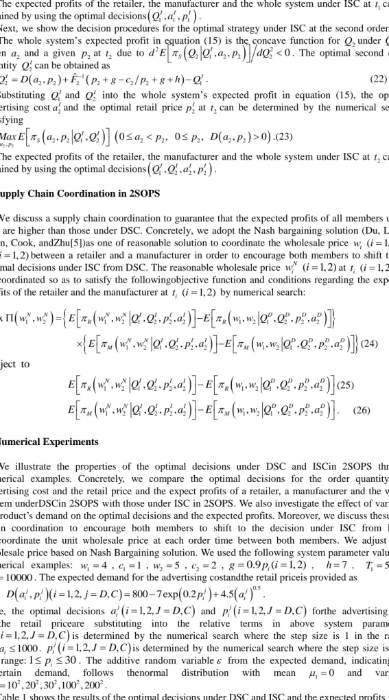
Table 1. Results of optimal decisions 2 Total order
Optimal decisions (jD I, ) Expected profits [ j]( , , , , )
k
E kR M S jD I
Order timet1 Order timet2 Order timet1 Order timet2
1 j Q 1 j a 1 j p 2 j Q 2 j a 2 j p R M S R M S DSC 102 600 555 201 19 105 622 18 3423 2230 5654 7575 2744 10320 202 663 565 242 19 98 616 18 3383 2285 5668 7430 2751 10181 302 667 570 249 19 97 615 18 3255 2318 5573 7283 2765 10049 1002 695 599 254 19 95 613 18 2243 2523 4767 6266 2873 9139 2002 731 636 226 19 95 579 18 809 2787 3596 4827 3017 7845 ISC 102 750 652 516 18 98 1149 17 3974 2614 6589 7448 3098 10546 202 757 670 647 18 87 1144 17 4022 2698 6720 7316 3114 10430 302 764 678 671 18 86 1142 17 3905 2740 6646 7171 3141 10313 1002 814 721 687 18 93 1140 17 2875 2980 5855 6147 3350 9498 2002 886 780 681 18 105 1128 17 1378 3309 4687 4692 3648 8341
retailer, a manufacturer and the whole system in 2SOPS when variance 2 in demand changes. First,
we compare the results of the optimal decisions under DSC and ISC in 2SOPS under variance in
demand 2 2
1 100
.From Table 1, we can see that the optimal order quantities Q1I and Q2Iat t1 and t2
under ISC are larger than Q1D and Q2D at t1 and t2 under DSC. This is clear from the condition
( 1, 2) ( 1, 2)
i i
c i w i in equations (16) and (20) at t1under DCS and (18) and (22)at t2under ICS We
can also see that the optimal advertising costs a1I and a2Iat t1 and t2 under ISC are higher than a1D and
2
D
a at t1 and t2under DSC. Also, it can be seen that the optimal retail prices p1I and p2Iat t1 and t2
under ISC are lower than p1D and p2Dat t1 and t2under DSC.This is the reason why ISC has the more
order quantity and no transaction cost regarding wholesales of product between the retailer and the
manufacturer from equations (17) and (21) at t1 and equations (19) and (23) at t2.
Next, as the sensitivity analysis, we discuss the effect of change of variance in demand2on the
optimal decisions under DSC and ISC as follows:
(i) Not only the optimal order quantities, Q1D and Q1I, under DSC and ISC at t1, but also the total order
quantities, Q1DQ2Dunder DSC and Q1IQ2I under ISC, increase as 2 increases. Meanwhile, the
optimal order quantities, Q2Dand Q2I, at t2 under DSC and ISChave neither increasing tendency nor
decreasing tendency as 2 increases.This is the reason why the optimal decisions
2
D
Q and Q2Iare
affected by each of the optimal expenditure costa iij( 1, 2,jD I, )at t ii( 1, 2), each of the
optimal retail price p iij( 1, 2,jD I, ) at t ii( 1, 2) and each of the expected demand
( ij, ij)( 1, 2, , )
D a p i jD I of product determined by a iij( 1, 2,jD I, )and ( 1, 2, , )
j i
p i jD I .
(ii) The optimal advertising costs, a1D anda1I at t1 tends to increase as 2 increasein the range of small
change(from 102 and 1002).However,
1
D
a and a1I at t1 tends to decrease as 2 increase in the range
of large change (more than 1002). The result is obtained in order to cover increase tendency of the
optimal order quantities, Q1Dand Q1I, att1as 2increases. Meanwhile, the optimal advertising costs,
2
D
a and a2I at t2 tends to decrease as 2 increase. The results are obtained in order to cover
decrease tendency of the optimal order quantities, Q2Dand Q2I, at t2as 2 increases.
(iii) All the optimal advertising costs under DSC and ISC, a iij( 1, 2,jD C, )at t ii( 1, 2)have no
change even if 2 increase. This is the reason why in this study, each advertising costat each order
time t ii( 1, 2)is dealt with the fixed cost having no relation with the quantity of product, not the
variable cost having relation with it. It implies that the impact of increase of 2is small for the unit
of product. This results in no change of the optimal decisions a iij( 1, 2,jD C, )at t ii( 1, 2).
From above results, we can verify the profitability by adjusting the optimaldecision for the product
order quantity, the advertising costand the retail price at the second order timet2.
Next, we discuss the effect of change of 2on the expected profits under DSC and ISC. The
expected profits of the retailer and the whole system decrease under DSC and ISC as 2increases.
Meanwhile, the expected profits of the manufacturer increase under DSC and ISC as 2 increases.
This is the reason why the total optimal order quantities under DSC and ISC increase as 2 increases.
Also, we compare the expected profits under DSCwith those under ISC. From Table 1, we can see that the expected profits of the manufacturer and the whole system under ISC are higher than those under DSC. Meanwhile, the expected profit of the retailer under ISC is lower than that under DSC. It is necessary to make supply chain coordination in order to encourage the retailer who is the leader of
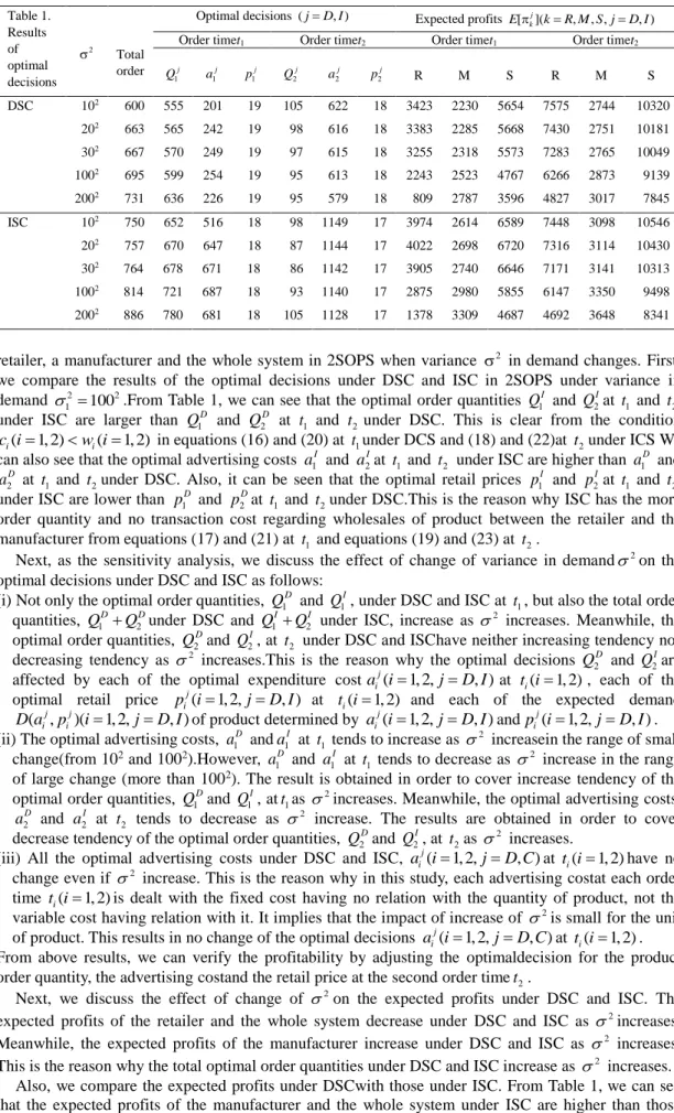
Table 2. Effect of supply chain
coordination Expected profit under DSC
Expected profit under ISC with supply chain coordination
2 w1 w2 1 N w 2 N w R M R M 102 5 7 4.0 11.2 7575 2744 7688 2857 202 5 7 3.7 14.3 7430 2751 7554 2876 302 5 7 4.4 8.9 7283 2765 7415 2897 1002 5 7 4.6 6.9 6266 2873 6445 3052 2002 5 7 3.4 15.2 4827 3017 5076 3265
thedecision-making under DSC to shift the decision-making under ISC from that under DSC. We
adoptedthe Nash bargainingsolutions wiN(i1, 2)at t ii( 1, 2)obtained from equations (24)-(26) into
the reasonable adjustments of the unit wholesale cost at t ii( 1, 2)between both members.
Table 2 shows the effect of supply chain coordination between the retailer and the manufacturer. From Table 2, it can be seen that the expected profits of both members under ISC with supply chain coordination are higher than those under DSC by adjusting the unit wholesale cost between both
members to N( 1, 2)
i
w i att ii( 1, 2). Thus, adjustments of the unit wholesale price at t ii( 1, 2)based
on Nash bargaining solution can bring to profitability to both members under ISC.
8.Conclusions and Future Research
In this study, we presented an optimal operation for2-stage-ordering-production system (2SOPS) consisting of a retailer and a manufacturer. We discussed the following 2SOPS into a supply chain: (1) a second-order opportunity for a retailer so as to reduce the uncertainty in demand of product and the shortage penalty cost of the unsatisfied demand, (2) two types of production mode for manufactures to respond to each ordering of the retailer with make-to-order policy. Also, we adopted two decisions for the order quantity, theadvertisingcost and the retail price. One wasmade under a decentralized supply chain(DSC) whose objective was to maximize the retailer’s profit. The other wasmade under an integrated supply chain(ISC) whose objective wasto maximize the whole system's profit. In the numerical analysis, we compared the results of the optimal decisions under DSC with those under ISC. Also, we discussedsupply chain coordinationto encourage both members to shift to the decisions under ISC from DSC. Wecoordinated the unit wholesale prices at each order time between both members under ISC. We adjusted each of the unit wholesale price based on Nash Bargaining solutions.
In this study, adjustments of the optimal decisions for product order quantity, the advertising cost and the retail price made based on the updated information of the demand distribution of product before the sales of product. In practice, it is necessary to keep adjusting these optimal decisions during the sales period of product. The relative modeling and discussions will be left as our future research.
Acknowledgements
This research has been supported by the Grant-in-Aid for Scientific Research C No. 25350451 fromthe Japan Society for the Promotion of Science.
References
[1] Weng, Z.K.Coordinating Order quantities between the Manufacturer and the Buyer: Generalized Newsvendor Model,
European Journal ofOperational Research, 156, 148-161. 2004
[2] Wang, S.D., Zhou, Y.W. and Wang, J.P.Supply Chain Coordination with Two Production Modes and Random Demand depending on Advertising Expenditure and Selling Price, International Journal of System Science, 41, 1257-1272. 2009
[3] Donohue, K.L. Efficient Supply Contracts for Fashion Goods with Farecast Updating and Two Production Modes,
Management Science, 46, 1397-1411. 2000
[4] Cachon, G.P. and Netessine, S.Sequential moves: Stackelberg Equilibrium Concept. In Simchi-Levi D, Wu S.D. and Shen Z.-J.editors.Handbook of Quantitative Supply Chain Analysis, Massachusetts, Kluwer Academic Publishers, 2004, p.40-41
[5] Du, J., Liang, L., Chen, Y., Cook, W.D. and Zhu, J. A Bargaining Game Model for Measuring Performance of Two-Stage Network Structures, European Journal ofOperational Research, 210, 390-397. 2011