Investigation of one-stage meta-analysis methods for joint longitudinal and time-to-event data through simulation and real data application

Investigation of one-stage meta-analysis methods for joint longitudinal and time-to-1

event data through simulation and real data application 2

Maria Sudell1,3, Ruwanthi Kolamunnage-Dona2,3 , François Gueyffier4, and Catrin

3

Tudur Smith2,3

4

Abstract 5

Background: Joint modelling of longitudinal and time-to-event data is often advantageous

6

over separate longitudinal or time-to-event analyses as it can account for study dropout, error

7

in longitudinally measured covariates, and correlation between longitudinal and time-to-event

8

outcomes. The current literature on joint modelling focuses mainly on the analysis of single

9

studies with a lack of methods available for the meta-analysis of joint data from multiple

10

studies. Methods: We investigate a variety of one-stage methods for the meta-analysis of

11

joint longitudinal and time-to-event outcome data. These methods are applied to the

12

INDANA dataset to investigate longitudinally measured systolic blood pressure, with each of

13

time to death, time to myocardial infarction and time to stroke. Results are compared to

14

separate longitudinal or time-to-event meta-analyses. A simulation study is conducted to

15

contrast separate versus joint analyses over a range of scenarios. Results: The performance of

16

the examined one-stage joint meta-analytic models varied. Models that accounted for

17

between study heterogeneity performed better than models that ignored it. Of the examined

18

methods to account for between study heterogeneity, under the examined association

19

structure, fixed effect approaches appeared preferable, whilst methods involving baseline

20

hazard stratified by study were least time intensive. Conclusions: One-stage joint

meta-21

analytic models that accounted for between study heterogeneity using a mix of fixed effects

22

or stratified baseline hazard were reliable, however models examined that included study

23

level random effects in the association structure were less reliable.

24

Keywords: Joint model, meta-analysis, longitudinal, time-to-event, simulation 25

1 _{Corresponding author,} 2 _{Joint senior author,} 3 _{Department of Biostatistics, University of} 26

Liverpool, 4 _{Centre Hospitalier Universitaire de Lyon} 27

1 Introduction 28

Univariate shared random effect joint models for longitudinal and time-to-event data

29

simultaneously model a single longitudinal and a single time-to-event outcome1_{. The model} 30

consists of a longitudinal sub-model and a time-to-event sub-model linked through an

31

association structure, which quantifies the relationship between the two outcomes. Many

32

options are presented in the literature for each sub-model (such as linear mixed effects

33

models or splines for the longitudinal sub-model, and proportional hazards or accelerated

34

failure time models for the time-to-event sub-model). A range of association structures

35

exist2, including sharing random effects between the sub-models3, sharing the current

36

longitudinal trajectory (both the fixed and random effects), or sharing the first derivative of

37

the longitudinal trajectory4. The research presented here focuses on joint models that concern

38

a single continuous longitudinal and a single possibly censored time-to-event outcome, linked

39

using an association structure consisting of shared zero mean random effects with common

40

association parameter for random effects acting at the same level3.

41

Joint models for longitudinal and time-to-event data are often employed to account for study

42

dropout and measurement error in time varying covariates, whilst producing less biased

43

estimates of study parameters3,5. An example of their application compared to separate

44

longitudinal models is presented by Powney et al6, who discuss the MAGNETIC trial7 which

reported a longitudinal case with missing data where a complete case analysis found no

46

significant difference between treatment groups, whilst use of joint models to account for

47

missing data resulted in a statistically significant difference. A recent review of current

48

reporting of single study joint analyses by Sudell et al8 identified that the number of

49

published joint analyses has been increasing over recent years, suggesting a growing resource

50

of joint datasets. Examples of single study joint models applied in the literature include

51

Jacoby et al9_{, Kolamunnage-Dona et al}10_{, Lloyd-Williams et al}11_{, and Kovanda et al}12_. 52

Glass13 defined meta-analysis (MA) as the statistical analysis or pooling of results from

53

several studies. Meta-analyses can result in analyses with increased precision and power,

54

whilst permitting new research questions to be answered. An individual participant or patient

55

data meta-analysis (IPD-MA) utilises the original data collected in each study, whereas an

56

aggregate data meta-analysis (AD-MA) utilises study level results, including those available

57

in published reports. IPD-MA can be one-stage or two-stage. A two-stage meta-analysis fits

58

models to the data from each study included in the meta-analysis, and then uses standard MA

59

techniques14,15 to pool the study specific parameter estimates. A one-stage meta-analysis

60

stores the data from all studies included in the meta-analysis in a single meta-dataset, to

61

which a single model is fitted (which should account for the clustering of data within studies).

62

The literature for meta-analyses is extensive14,15, but research into the meta-analysis of joint

63

longitudinal and time-to-event data is limited to a small number of references8,16_{. However, it} 64

is reasonable that if joint modelling is preferred over separate longitudinal or time-to-event

65

models in certain single study cases (e.g. to account for informative dropout in longitudinal

66

study designs17 or when a time-to-event outcome is influenced by longitudinal outcomes18),

67

use of joint models rather than separate methods may also be preferred in a meta-analytic

68

setting.

69

Currently, methodological research has mainly focused on joint models applied to single

70

study datasets (for overviews see5,19), although a limited number of references exist that deal

71

with multi-centre joint data20, and multi-level joint models21. However, these references did

72

not specifically investigate the meta-analytic case. Multi-centre and meta-analytic datasets

73

are similar, in that they have a structure where individuals are nested within studies or

74

centres. However, the number of higher level units differs between cases; meta-analyses

75

often contain fewer studies, each containing a larger number of individuals, whereas

multi-76

centre datasets often contain a larger number of centres, each containing a comparatively

77

smaller number of individuals. As such, the spread of data across the different levels is

78

different for a meta-analytic compared to a multi-centre dataset, leading to potentially

79

different approaches being required. This paper extends this methodology by investigating

80

multi-level joint models specifically for use in meta-analytic datasets.

81

Recently Sudell et al16 investigated methods for the two-stage MA of joint data. In this

82

article, we investigate one-stage models to analyse individual participant multi-study joint

83

longitudinal and time-to-event data (termed joint IPD). The results of the one-stage

meta-84

analytic joint models are compared to one-stage separate longitudinal or time-to-event

meta-85

analytic models. The article begins with a discussion of the methods employed in the

86

investigation. The presented methods are then applied to an example dataset. A simulation

87

study is then conducted to test the methods under a range of scenarios. The article concludes

88

with a discussion of joint modelling methodology in one-stage MA.

2 Methods for one-stage joint IPD-MA 90

As mentioned, this research assumes the availability of joint longitudinal and time-to-event

91

IPD. This IPD is considered to have three nested levels, namely longitudinal measurements at

92

level 1, nested within individuals at level 2, nested within studies at level 3. The joint models

93

considered in this research assume a linear mixed effects model for the longitudinal outcome,

94

and a Cox Proportional Hazards (PH) model with an unspecified baseline hazard for the

time-95

to-event outcome. The two sub-models are linked through shared zero mean random effects,

96

with common association parameter (represented using 𝜶 terms) for the random effects acting

97

at the same level. Unlike joint models for single study data, the proposed models must

98

account for the clustering of individuals within studies, and model potential heterogeneity

99

between these studies.

100

The one-stage joint model follows the structure:

101 𝑌𝑘𝑖𝑗 = 𝑿𝟏𝜷𝟏+ 𝒁𝒌𝒊(𝟐)𝒃𝒌𝒊(𝟐)+ 𝒁𝒌(𝟑)𝒃𝒌(𝟑)+ 𝜀𝑘𝑖𝑗 𝜆𝑘𝑖(𝑡) = 𝜆0(𝑡) exp(𝑿𝟐𝜷𝟐+ 𝑊2𝑘𝑖(𝑡)) 𝑊_2𝑘𝑖(𝑡) = 𝛼(2)_(𝑍 𝑘𝑖(2)𝑏𝑘𝑖(2)) + 𝛼(3)(𝑍𝑘(3)𝑏𝑘(3)) (1)

Studies are identified by 𝑘 = 1 … 𝐾, where 𝐾 is the total number of studies in the

meta-102

dataset. Individuals within each study are represented by 𝑖 = 1 … 𝑛_𝑘 where 𝑛_𝑘 denotes the

103

total number of individuals in study 𝑘. The longitudinal measurement points are identified

104

using 𝑗 = 1 … 𝑚𝑘𝑖 where 𝑚𝑘𝑖 represents the total number of longitudinal measurements

105

recorded for individual 𝑖 in study 𝑘.

106

The longitudinal measurement recorded for individual 𝑖 in study 𝑘 at time-point 𝑗 is

107

represented by 𝑌_𝑘𝑖𝑗, with the longitudinal error term 𝜀_𝑘𝑖𝑗. Fixed effects are represented using

108

𝜷 terms, with the first element of the subscript identifying the sub-model they belong to (such

109

that 𝜷_𝟏= 𝛽₁₁, 𝛽₁₂, 𝛽₁₃, … are the longitudinal sub-model fixed effects, and 𝜷_𝟐=

110

𝛽₂₁, 𝛽₂₂, 𝛽₂₃, … are the time-to-event sub-model fixed effects). Random effects are

111

represented by 𝒃, with individual level (level 2) random effects represented by 𝒃_𝒌𝒊(𝟐) and study

112

level (level 3) random effects by 𝒃_𝒌(𝟑). Design matrices are represented by 𝑿 for the fixed

113

effects and 𝒁 for the random. 𝑿_𝟏 represents the longitudinal sub-model fixed effects design

114

matrix, and 𝑿_𝟐 represents the time-to-event sub-model fixed effects design matrix.

115

Additionally, 𝒁_𝒌𝒊(𝟐) represents the design matrix for the individual level (level 2) random

116

effects, and 𝒁_𝒌(𝟑) represents the design matrix for the study level (level 3) random effects.

117

The individual level random effects follow distribution 𝒃_𝑘𝑖(2)~𝑁(𝟎, 𝑫), whilst the study level

118

random effects follow distribution 𝒃_𝑘(3)~𝑁(𝟎, 𝑨), and the error terms each follow distribution

119

𝜀𝑘𝑖𝑗~𝑁(0, 𝜎𝑒2). The individual level and the study level random effects are considered

120

independent of each other, and of the error terms. The random effects are intended to

121

represent how covariate effects differ for units at the respective levels (individuals or studies)

122

from those estimated for the overall population by the fixed effects, for example how the

123

individuals contained within a particular study differ from those in the overall population. As

124

such, the 𝒁 matrices are assumed to be subsets of the 𝑿_𝟏 matrix.

125

In the time-to-event sub-model, 𝜆0(𝑡) represents the unspecified baseline hazard. The

sub-126

models are linked through shared zero mean random effects, with common association

127

parameters 𝛼(2) for the individual level random effects and 𝛼(3) for the study level random

effects. Note that if a particular component of the joint model is not required (e.g. the study

129

level random effects), terms involving this component (e.g. 𝒁_𝒌(𝟑)𝒃_𝒌(𝟑)) do not appear in the

130

model.

131

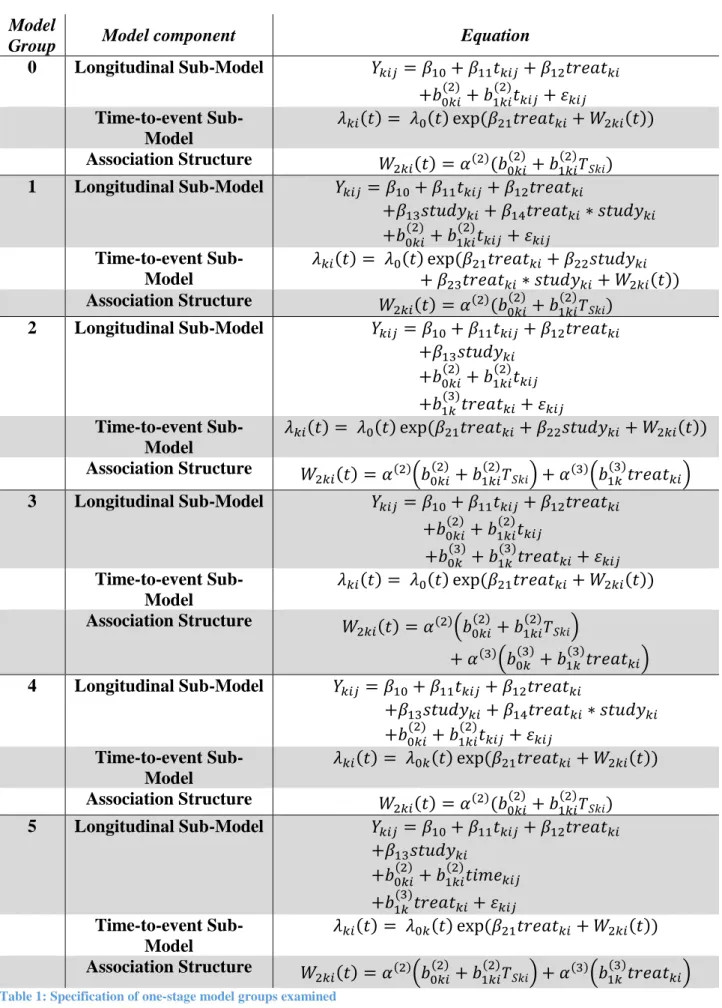
A range of model groups are investigated, which represent a variety of methods to account

132

for between study heterogeneity. The specifications of the model groups are stated in Table

133

1. These models involve only longitudinal time (𝑡_𝑘𝑖𝑗), a binary treatment assignment variable

134

(𝑡𝑟𝑒𝑎𝑡_𝑘𝑖), and study membership (𝑠𝑡𝑢𝑑𝑦_𝑘𝑖) as covariates. However, the models examined

135

can be easily extended if other covariates are of interest to the MA. Note, instances of

136

longitudinal time 𝑡_𝑘𝑖𝑗 in the association structure term 𝑊_2𝑘𝑖(𝑡) (which is present in the

time-137

to-event sub-model) are replaced by the individuals survival time 𝑇_𝑆𝑘𝑖.

138

Model group 0 in Table 1 is a naïve model which does not account for between study

139

heterogeneity in any way. This model is presented here to highlight the consequence of

140

ignoring the clustered nature of multi-study joint data. Note, any instances of longitudinal

141

time in the association structure are replaced with the individual’s survival time

142

(denoted 𝑇_𝑆𝑘𝑖, equal to the minimum of their event and censoring times).

143

Model group 1 accounts for between study heterogeneity using a fixed study membership

144

variable, along with its interaction with treatment assignment, in both sub-models. Study

145

membership is expected to be a factor variable, and so a separate 𝛽13, 𝛽14, 𝛽22 and 𝛽23

146

parameter will be produced for each study 𝑘 in the meta-analysis (apart from the reference or

147

baseline study), denoted 𝛽_13𝑘, 𝛽_14𝑘, 𝛽_22𝑘 and 𝛽_23𝑘. The study considered to be the reference

148

study should be representative of the population of interest. In model group 1, inclusion of

149

the fixed study membership variable allows calculation of study specific fixed longitudinal

150

trajectory intercepts (with 𝛽₁₀ representing the fixed intercept for the reference study, and

151

𝛽10+ 𝛽14𝑘 for non-reference study 𝑘). Likewise, study specific longitudinal treatment

152

effects can be calculated (with 𝛽₁₃ representing the fixed longitudinal treatment effect for the

153

reference study, and 𝛽₁₃+ 𝛽_15𝑘 for non-reference study 𝑘). In the time-to-event sub-model,

154

the 𝛽_22𝑘 parameter represents the difference in risk of an event between study 𝑘, and the

155

reference study. The deviation in risk of an event due to treatment group is equal to 𝛽₂₁ for

156

the reference study, and by 𝛽₂₁+ 𝛽_23k for non-reference study 𝑘.

157

Model group 2 accounts for between study heterogeneity using a fixed study membership

158

variable in both sub-models, and a study level zero-mean random treatment effect (𝑏_1𝑘(3)).

159

Study specific longitudinal trajectory intercepts and log-hazard ratio risks of an event for

160

each study can be calculated from the fixed effects as for model group 1. The interpretation

161

of the study specific random treatment effect 𝑏_1𝑘(3)is more complex than for separate

162

longitudinal or time-to-event one-stage MA-models due to its presence in both sub-models.

163

In the longitudinal sub-model, the 𝑏_1𝑘(3) term adjusts the overall population treatment effect

164

coefficient 𝛽₁₂ to give the observed treatment effect in study 𝑘 of 𝛽₁₂+ 𝑏_1𝑘(3). Through the

165

association structure, 𝑏_1𝑘(3) is present in the time-to-event sub-model. As such, the population

166

treatment effect coefficient 𝛽21 is altered to give a study specific estimate of the deviation in

167

the risk of an event due to treatment group (𝛽₂₁+ 𝛼(3)𝑏_1𝑘(3)).

168

Model group 3 accounts for between study heterogeneity solely using study level random

169

effects, as it involves a study level random intercept (𝑏_0𝑘(3)) and random treatment effect

170

(𝑏_1𝑘(3)). Again, the interpretation of these random effects is more complex than for separate

one-stage longitudinal or time-to-event MA-models due to their presence in both sub-models

172

through the association structure. The study level random intercept 𝑏_0𝑘(3) causes the

173

longitudinal intercept for study 𝑘 to equal 𝛽₁₀+𝑏_0𝑘(3), but also 𝛼(3)𝑏_0𝑘(3) represents the deviation

174

in the risk of an event in the 𝑘th study from the population average taken across all studies in

175

the meta-analysis. The interpretation of the random treatment effect (𝑏_1𝑘(3)) is the same as for

176

model group 2.

177

Model group 4 has a longitudinal sub-model with the same specification (and so

178

interpretation) as model group 1. However the baseline hazard in the time-to-event sub-model

179

is stratified by study (𝜆_0𝑘(𝑡)), and the time-to-event sub-model contains only a fixed

180

treatment assignment term. As such, between study heterogeneity in the time-to-event model

181

is captured by the study specific baseline hazards.

182

Model group 5, accounts for between study heterogeneity in a variety of ways. A fixed study

183

membership term is included in the longitudinal sub-model, a study level random treatment

184

effect (𝑏_1𝑘(3)) is present in both sub-models through the association structure, and the baseline

185

hazard of the time-to-event sub-model is stratified by study. Each component of the model

186

has interpretations as already discussed.

187

In addition to the one-stage joint MA-models, we also fit separate longitudinal and

time-to-188

event one-stage MA-models for the comparison with the joint estimates. These separate

189

models have the same specification as the corresponding joint model sub-models, except for

190

the 𝑊_2𝑘𝑖(𝑡) term is removed from the time-to-event one-stage MA-models.

191

3 Model fitting 192

The models described in Section 2 were fitted using the Expectation Maximisation (EM)

193

algorithm22, whose use in single study joint modelling analyses has been described by

194

Wulfsohn and Tsiatis1 and Rizopoulos4. Starting values for the algorithm were extracted from

195

initial separate longitudinal and time-to-event model fits (of the same specification as the

196

corresponding sub-models of the joint model, excluding the association structure). In the

197

Expectation or E-step, estimates of functions of random effects were calculated using

pseudo-198

adaptive Gaussian quadrature procedures23, where conditional modes of the random effects

199

calculated in the initial separate longitudinal model fit were used to calculate appropriate

200

locations for the abscissa to be used throughout the model fitting process. In the

201

Maximisation or M-step, these estimated functions of the random effects were used to

202

calculate maximum likelihood estimates of model parameters. The derived maximum

203

likelihood estimators have been made available as Supplemental Material.

204

4 Software 205

We developed a flexible R24 code to fit one-stage multi-study joint models described in this

206

article which will be available as joineRmeta package, the R codes can currently be

207

downloaded at https://github.com/mesudell/joineRmeta/. This software is an extension of the

208

single study joint modelling package joineR25 to the multi-study case. Example code and

209

simulated data are available in the supplemental information, demonstrating methods

210

discussed in this article.

5 Application 212

5.1 Example Data 213

To investigate the behaviour of the proposed methods in a real world scenario, the methods

214

were applied to a subset of the INDANA dataset26. This is a multi-study dataset compiled to

215

investigate the effect of patient characteristics on the efficacy of pharmacological treatment

216

for high blood pressure. The subset analysed here (henceforward referred to as the INDANA

217

dataset) contains any study identified by the INDANA collaboration26 _{that supplied both} 218

longitudinal and time-to-event data, and contains 6 studies (EWPHE27, COOP28, STOP29,

219

SHEP30, MRC131 and MRC232 ). The INDANA dataset concerns hypertensive patients

220

assigned to one of two treatment groups; any treatment for hypertension versus placebo, no

221

treatment or usual care. Longitudinally measured Systolic and Diastolic Blood Pressure were

222

available, referred to as SBP and DBP. Three time-to-event outcomes were measured,

223

namely time to death, time to myocardial infarction (MI) and time to stroke.

224

The data contained 9 possible longitudinal time-points at baseline, 6 months, 1 year and

225

annually thereafter to a maximum of 7 years. The SHEP study recorded individuals at only 6

226

measurement times, whilst STOP and MRC1 presented 7 measurement times, with the

227

remaining studies presenting data at each of the 9 possible measurement times. Only

228

longitudinal data recorded prior to an individual’s survival time contributed to the analyses.

229

Tables of the number of measurements provided by each study at each time point are

230

available in the supplemental information (supplemental tables S1-S3).

231

Analyses of SBP and each time-to-event outcome are presented in Tables 2-4. For EWPHE,

232

an intention to treat analysis was only possible for fatal endpoints, and so the study only

233

contributes to the analysis of SBP and time to death. As such, the final dataset examined

234

contained a maximum of 6 studies totalling at most 29825 individuals. The exact number of

235

individuals involved in each analysis is stated in the captions of Tables 2-4.

236

The aim of this investigation was to illustrate the proposed one-stage joint meta-analytic

237

models, rather than to investigate potential treatment modifiers. As such, whilst the

238

INDANA dataset contained a range of patient covariates that could influence the outcomes,

239

models in this investigation included only treatment assignment, study membership and the

240

longitudinal time covariate.

241

The models of specification shown in Table 1 were fitted to the data for each combination of

242

outcomes (SBP and each of time to death, time to MI and time to stroke, with longitudinal

243

outcome 𝑌_𝑘𝑖𝑗 = 𝑆𝐵𝑃_𝑘𝑖𝑗). However plots of the longitudinal trajectories for each study

244

panelled by event type (Supplemental Figures S1-S3) indicated a changepoint early in the

245

trajectories. A range of terms were tested to account for non-linearity due to the changepoint

246

including 𝑡_𝑘𝑖𝑗2 , exp (−𝑡𝑘𝑖𝑗) and exp (−𝑎 ∗ 𝑡𝑘𝑖𝑗). Comparison of the log-likelihoods and AIC

247

values of the models determined that inclusion of the term exp (−3 ∗ 𝑡_𝑘𝑖𝑗) gave the best fit.

248

Consequently, in addition to the terms stated in Table 1, each longitudinal sub-model also

249

contained a exp (−3 ∗ 𝑡_𝑘𝑖𝑗) term (for clarity, full model specifications for real data analyses

250

are available in Supplemental Table S4).

251

In the models examined, a statistically significant negative treatment assignment coefficient

252

in the time-to-event model would indicate that assignment to any treatment for hypertension

253

versus placebo, no treatment or usual care significantly reduced the risk of the event in

254

question. Model groups 0, 2, 3, 4 and 5 each produce a single global time-to-event treatment

effect estimate (𝛽₂₁), whilst model group 1 produces study specific treatment effect estimates

256

(calculated by 𝛽21 for the reference study, and 𝛽21+ 𝛽23𝑘 for non-reference study 𝑘).

257

A statistically significant negative treatment assignment coefficient in the longitudinal

sub-258

model would indicate that assignment to any treatment for hypertension significantly

259

decreased SBP. Model groups 0, 2, 3 and 5 each produce a single global longitudinal

260

treatment effect estimate (𝛽₁₂), whilst model groups 1 and 4 produce study specific estimates

261

(calculated by 𝛽₁₂ for the reference study, and 𝛽₁₂+ 𝛽_14𝑘 for non-reference study 𝑘).

262

A statistically significant positive study level association parameter (𝛼(3)) indicates that

263

individuals in studies with longitudinal outcome values above the corresponding overall

264

population mean are at higher risk of experiencing the event at a given time point. A

265

statistically significant positive individual level association parameter (𝛼(2)) indicates that

266

individuals with longitudinal values above that predicted by the terms in the longitudinal

sub-267

model (apart from the individual level random effects) are at higher risk of experiencing the

268

event at a given time point. Association parameters were only estimated for joint analyses.

269

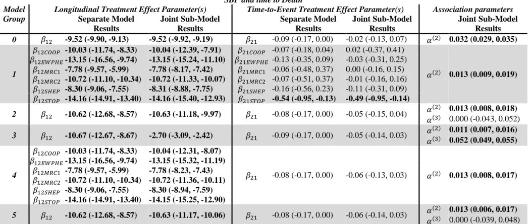
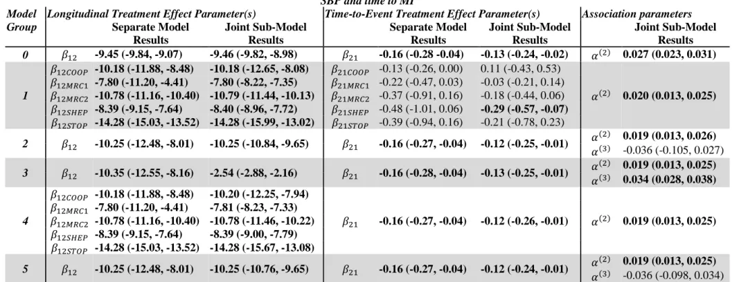
5.2 Results from the INDANA dataset meta-analyses 270

Tables 2-4 present the results of application of model groups 0-5 (as stated in Supplemental

271

Table S4) to the INDANA dataset. Graphical representations of these results are shown in

272

Supplemental Figures S4-S12.

273

Across all pairwise combinations of outcomes investigated, the estimated treatment effect

274

from the separate longitudinal one-stage IPD-MA and the joint one-stage IPD-MA

275

longitudinal sub-model were significant and negative, indicating that assignment to treatment

276

for hypertension significantly reduced SBP compared to placebo, no treatment or usual care.

277

The estimated treatment effect from the separate and joint analyses agreed well across model

278

groups examined, apart from model group 3 (which solely accounted for between study

279

heterogeneity using study level random effects). Here the separate results were similar to

280

those produced by the other model groups, however the results from the joint analysis, whilst

281

still significant, were much smaller in magnitude than the joint results from the other

282

modelling groups. In the separate group 3 model, the study level random effects accounted

283

for between study heterogeneity in the longitudinal trajectory. However, in the joint model

284

they also accounted for between study heterogeneity in the time-to-event sub-model through

285

their presence in the association structure. It was important to determine if sharing study

286

level random effects in this way between sub-models caused bias in covariate estimates,

287

examined through simulations in Section 5.

288

Throughout the analyses, the estimated time-to-event treatment coefficient from the joint

one-289

stage IPD-MA models were smaller in magnitude than those from the separate one-stage

290

IPD-MA model. However the direction of the results agreed between the separate and the

291

joint analyses. For SBP and time to death, the separate and joint analyses agreed in the

292

significance of results, with a significant reduction in risk of death due to assignment to any

293

treatment for hypertension estimated only for the STOP trial for model group 1. For SBP and

294

time to MI, model groups 0, 2, 3, 4 and 5 for both the separate and joint analyses estimated

295

significant negative global treatment effect estimates, indicating a significant reduction in risk

296

of MI due to assignment to treatment for hypertension. However, for model group 1, only the

297

study specific estimate for the SHEP trial from the joint analysis was significant. For SBP

298

and time to stroke, model groups 0, 2, 3, 4 and 5 for both the separate and joint analyses

299

estimated significant negative global treatment effect estimates, indicating a significant

300

reduction in risk of stroke due to assignment to treatment for hypertension. These treatment

assignment coefficients were larger in magnitude than the results for time to death or time to

302

MI. For model group 1, the separate time-to-event model identified study specific significant

303

treatment effects for COOP and MRC1, however the joint analysis additionally identified

304

significant effects for SHEP and STOP.

305

Individual level random effects were included in all model groups examined causing the

306

individual level association parameter 𝛼(2) to be present in all model groups. For each set of

307

outcomes examined, all model groups estimated significant positive values for 𝛼(2),

308

indicating that individuals with SBP values above the corresponding population average are

309

at higher risk of an event. We should note that model group 0 consistently estimated

310

𝛼(2)values of larger magnitude than the other model groups (which were consistent in the

311

magnitude of 𝛼(2) estimated). This highlights the importance of accounting for between

312

study heterogeneity in joint analyses of multi-study data.

313

Study level random effects were only employed in model groups 2, 3 and 5, meaning that the

314

study level association parameter 𝛼(3) was only estimated in these model groups. There was

315

a noticeable discrepancy between results from model group 3, and model groups 2 or 5.

316

Model group 3 contained both a study level random intercept and treatment effect, whereas

317

model groups 2 and 5 contained only a study level random treatment effect. Model group 3

318

estimated a significant positive study level association parameter across all three sets of

319

analyses (with interpretation that studies with SBP values above the population average were

320

at higher risk of an event). However as noted earlier, for the joint analysis, estimated

321

parameters from model group 3 were inconsistent with the results produced by the other

322

model groups. Model groups 2 and 5 estimated insignificant 𝛼(3) values across the three sets

323

of analyses, which were different in magnitude to model group 3, and had wide confidence

324

intervals. These results motivated a simulation study to investigate when use of shared study

325

level random effects may be recommended.

326

6 Simulation Investigations 327

In practice meta-analyses involve data with very different characteristics to those displayed in

328

our real data example. For example, associations between the longitudinal and time-to-event

329

outcomes may be different in significance and / or magnitude. The number of studies

330

included in the meta-analysis might differ. There might be a different level of variability or

331

heterogeneity between studies involved in the meta-analysis. To assess the behaviour of the

332

models stated in Table 1 under a range of these different conditions, a range of simulation

333

investigations were conducted. These simulations can be split into three main sets:

334

Simulation Set 1 investigates the models under different levels of association, Simulation Set

335

2 investigates differing numbers of studies included in the meta-analysis, and Simulation Set

336

3 investigates differing levels of between study heterogeneity. During the simulation

337

investigations data was firstly simulated using the models and methods discussed in Section

338

6.1. The models stated in Table 1 were then fitted to each simulated dataset, the results of

339

which are presented in Section 6.2.

340

6.1 Data Simulation 341

Data for each set of simulations was simulated under the same model structure, but with

342

different model parameter values, which we will now describe. For each set of simulations,

343

for each scenario, 1000 datasets were simulated.

344

For each dataset within each set of simulations, multi-study joint data was generated

345

containing a single continuous normally distributed longitudinal outcome and a single

346

censored time-to-event outcome. The number of included studies varies between simulation

sets, however each simulated study contained 500 individuals randomised equally to two

348

treatment groups. A maximum of 10 longitudinal measurements at times 0, 0.25, 0.5, 1, 1.5,

349

2, 2.5, 3, 3.5, 4 were permitted, with measurements recorded only up to the individual’s

350

survival time (𝑇𝑆𝑘𝑖). Data for all studies was simulated simultaneously, with any between

351

study heterogeneity generated through specification of the distribution of study level random

352

effects. The longitudinal data was simulated under equation (2):

353

𝑌_𝑘𝑖𝑗 = 𝛽₁₀+ 𝛽₁₁𝑡_𝑘𝑖𝑗+ 𝛽₁₂𝑡𝑟𝑒𝑎𝑡_𝑘𝑖+ 𝑏_0𝑘𝑖(2) + 𝑏_1𝑘𝑖(2)𝑡_𝑘𝑖𝑗 + 𝑏_0𝑘(3)+ 𝑏_1𝑘(3)𝑡𝑟𝑒𝑎𝑡_𝑘𝑖 + 𝜀_𝑘𝑖𝑗 (2) In equation (2), the longitudinal outcome 𝑌_𝑘𝑖𝑗 follows a linear mixed effects model containing

354

fixed intercept, time and treatment assignment terms (with coefficients 𝛽₁₀, 𝛽₁₁ and 𝛽₁₂),

355

individual level random intercept and slope terms (𝑏_0𝑘𝑖(2) and 𝑏_1𝑘𝑖(2)), study level random

356

intercept and treatment effect terms (𝑏_0𝑘(3) and 𝑏_1𝑘(3)) and an error term 𝜀_𝑘𝑖𝑗. The random

357

effects follow multivariate normal distributions, with individual level random effects

358

distributed 𝒃_𝑘𝑖(2)~𝑁(𝟎, 𝑫), and study level random effects distributed 𝒃_𝑘(3)~𝑁(𝟎, 𝑨). The

359

random effects are independent of each other, and of the error terms, which are considered to

360

be independently and identically distributed 𝜀_𝑘𝑖𝑗~𝑁(0, 𝜎_𝑒2).

361

The simulation of time-to-event data under a proportional hazards model with time varying

362

covariates is described by Bender et al33 and Austin34. In these simulations, the time-to-event

363

data was generated under equation (3), where 𝜆₀(𝑡) is an unspecified baseline hazard:

364

𝜆𝑘𝑖(𝑡) = 𝜆0(𝑡) exp(𝛽21𝑡𝑟𝑒𝑎𝑡𝑘𝑖+ 𝑊2𝑘𝑖(𝑡))

𝑊2𝑘𝑖(𝑡) = 𝛼(2)𝑊1𝑘𝑖(𝑡) = 𝛼(2)(𝑏0𝑘𝑖(2) + 𝑏1𝑘𝑖(2)𝑇𝑆𝑘𝑖) + 𝛼(3)(𝑏0𝑘(3)+ 𝑏1𝑘(3)𝑡𝑟𝑒𝑎𝑡𝑘𝑖)

(3)

As a time varying covariate is present in the time-to-event sub-model (the individual level

365

random time term 𝑏_1𝑘𝑖(2), present through the association structure), event times are simulated

366

under a Gompertz distribution, as it has a baseline hazard that can vary over time.

367

Consequently, individual event times 𝑇_𝐸𝑘𝑖 are generated under equation (4), (where

368 𝒁_𝒌𝒊(𝟑)𝒃_𝒌(𝟑) = 𝑏_0𝑘(3)+ 𝑏_1𝑘(3)𝑡𝑟𝑒𝑎𝑡𝑘𝑖): 369 𝑇𝐸𝑘𝑖 =_𝛼(2)𝒃1 𝟏𝒌𝒊 (𝟐)_+𝜃 1log [1 + (𝛼(2)𝑏_1𝑘𝑖(2)+𝜃1)(− log(𝑈𝑘𝑖)) exp(𝜃0+𝛽21𝑡𝑟𝑒𝑎𝑡𝑘𝑖 +𝛼(2)𝑏0𝑘(2)+𝛼(3)(𝒁𝒌𝒊(𝟑)𝒃𝒌(𝟑))) ] (4)

In equation (4), 𝑈_𝑘𝑖 is an individual specific realisation from a Uniform 𝑈(0,1) distribution.

370

The parameters 𝜃₀ (the exponential of which is the scale parameter of a Gompertz

371

distribution) and 𝜃₁ (the shape parameter of a Gompertz distribution) are used along with the

372

coefficients in the model to control the distribution of the event times.

373

The event times 𝑇_𝐸𝑘𝑖 were specified to be Gompertz distributed with mean 𝜇₀ = 3 and

374

standard deviation 𝜎₀ = 0.5. Using the extreme value distribution (as recommended by

375

Bender et al33_{, with 𝛾 ≈ 0.5772 representing Euler’s constant), this lead to the parameters} 376

controlling the event times distributions to be set to:

377 𝜃₁ = 𝜋 √6𝜎0 = 𝜋 (0.5)√6 ≈ 2.5651 378

𝜃₀ = log(𝜃₁exp(−𝛾 − 𝜇₀𝜃₁)) = log(𝜃₁exp(−𝛾 − 3𝜃₁)) ≈ −7.330517 379

A Gompertz distribution has increasing hazard for a positive shape parameter, constant

380

hazard for a shape parameter equal to 0 (equivalent to an exponential distribution), and a

381

decreasing hazard for negative shape parameters. Under the above model, the probability

382

density function of the event times takes form:

383

𝑓₀(𝑡) = 𝜅 exp(𝜃1𝑡) exp (_𝜃𝜅

1(1 − exp(𝜃1𝑡))), where 𝜅 = exp 𝜃0

(5)

If the shape parameter is negative, if time is allowed to tend towards infinity, there is a

non-384

zero probability of living forever. As such, in the function used to simulate event times

385

(available in the aforementioned joineRmeta package), when the Gompertz distribution is

386

employed event times are simulated under a two step process. First, for each individual 𝑖

387

within study 𝑘, the following two conditions are checked (using the realization from the

388 𝑈(0,1) distribution, 𝑈_𝑘𝑖). 389 𝐶𝑜𝑛𝑑𝑖𝑡𝑖𝑜𝑛 1: (𝜃₁ + 𝛼(2)_𝑏 1𝑘𝑖(2)) < 0 390 𝐶𝑜𝑛𝑑𝑖𝑡𝑖𝑜𝑛 2: 𝑈𝑘𝑖 < exp ( exp (𝜃0+ 𝛼(2)𝑏0𝑘𝑖(2)) 𝜃₁ + 𝛼(2)_𝑏 1𝑘𝑖(2) ) 391

If the conditions are both true, the individual is automatically assigned an event time of

392

infinity, otherwise their event time is generated under equation (4).

393

The censoring times were simulated under an exponential distribution with parameter 𝜆_{𝑐𝑒𝑛𝑠}.

394

As such, individual censoring times 𝑇_𝐶𝑘𝑖 are generated using equation:

395

𝑇𝐶𝑘𝑖 =

−log(𝑈𝑘𝑖) 𝜆𝑐𝑒𝑛𝑠

(6)

The event rate of the simulated data was controlled through the censoring process. Due to the

396

volume of planned simulations, only datasets with a “low” (~25%) event rate were generated.

397

A range of censoring parameters were tested to obtain datasets with mean event rate at 25%,

398

leading to setting 𝜆_{𝑐𝑒𝑛𝑠} = exp(−0.426). The survival time for each individual was the

399

minimum of their censoring and event times (𝑇_𝑆𝑘𝑖 = min (𝑇_𝐸𝑘𝑖, 𝑇_𝐶𝑘𝑖)).

400

All data used in the simulation studies were simulated under the models shown in equations

401

(2) and (3), although certain parameter values were altered between different sets of

402

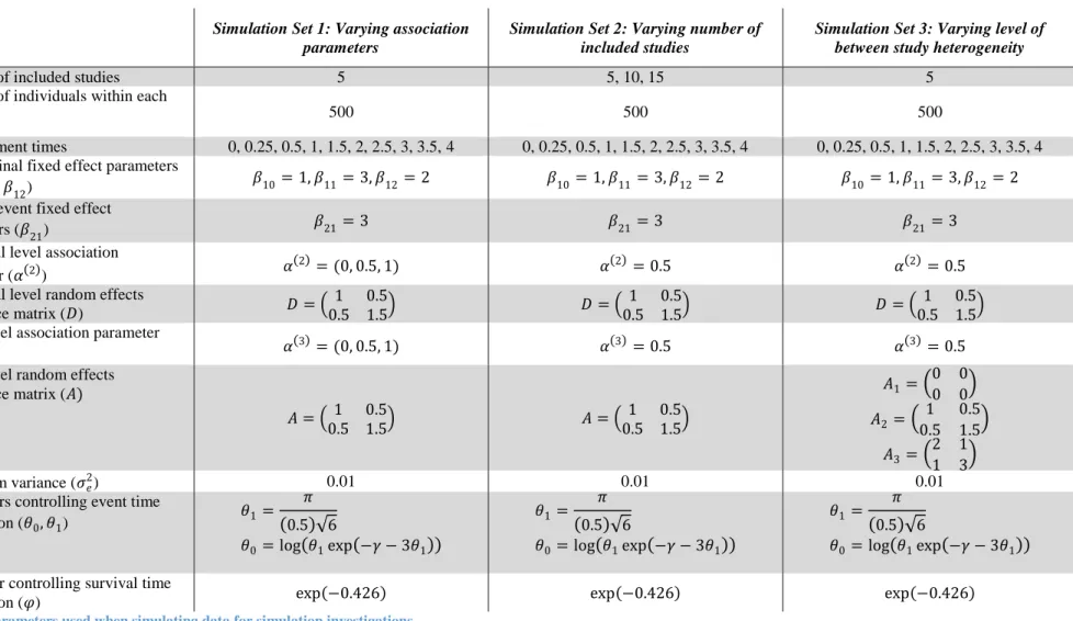
simulations. Parameter values in the simulation sets were chosen such that deviations of

403

different methods from the true parameters values would be clearly discernible. A summary

404

of the values used for the different sets of simulations is given in Table 5. All simulation

405

groups utilised the same fixed effect and error term variance values (𝛽₁₀= 1, 𝛽₁₁ = 3, 𝛽₁₂=

406

2, 𝛽₂₁= 3, 𝜎_𝑒2 = 0.01). Additionally, throughout different sets of simulations, the individual

407

level random effects covariance matrix 𝑫 remained constant (defined in Table 5). However

408

the remaining aspects of the datasets (association parameters, number of included studies,

409

level of between study heterogeneity) varied between simulation sets. These aspects are

410

stated in Table 5, and are briefly discussed in the following sections. Throughout, both

411

separate longitudinal or time-to-event one stage MA and joint one stage MA were conducted,

412

to compare the two approaches,

6.1.1 Simulation Set 1: Varying levels of association 414

In practice, the magnitude of the association between the longitudinal and time-to-event

415

outcomes at the individual and the study level of the data could impact the performance of the

416

model groups defined in Section 2. Consequently, we performed a simulation investigation

417

to assess the effect of varying magnitudes of association at different levels.

418

The individual level association parameter 𝛼(2) and the study level association parameter 𝛼(3)

419

were permitted to take values 0, 0.5 and 1, giving a total of 9 unique scenarios. The number

420

of included studies in each dataset equalled 5, whilst the study level random effects

421

covariance matrix 𝑨 (Table 5) remained constant across scenarios.

422

6.1.2 Simulation Set 2: Varying numbers of studies included in the meta-analysis 423

The models introduced in Section 2 that include study level random effects may not reliably

424

estimate the distribution of the study level random effects unless the number of studies

425

included in the meta-analysis is large. In addition, models including fixed interaction terms

426

between study membership and treatment group may become unwieldy or difficult to

427

estimate as the number of included studies increases. To investigate this, simulations were

428

conducted comparing one-stage analyses of joint data for datasets containing 5, 10 or 15

429

studies.

430

During this set of simulations, the association parameters were held constant across scenarios

431

(with 𝛼(2) = 𝛼(3) = 0.5). Additionally, the study level random effects covariance matrix 𝑨

432

(Table 5) remained constant across scenarios.

433

6.1.3 Simulation Set 3: Varying levels of between study heterogeneity 434

Finally, the level of between study heterogeneity could affect the behaviour of the different

435

one-stage models described in Section 2. As such, the third set of simulations alters the study

436

level random effects covariance matrix 𝑨 across different scenarios, to increase or reduce

437

between study heterogeneity. Values taken for 𝑨, labelled 𝑨𝟏, 𝑨𝟐 and 𝑨𝟑 are specified in

438

Table 5, representing cases for no between study heterogeneity, and then two increasing

439

levels of between study heterogeneity.

440

During this simulation set, across all scenarios 5 studies were simulated for each dataset, with

441

association parameters held constant across scenarios at 𝛼(2) = 𝛼(3)= 0.5.

442

6.1.4 Models fitted to Simulated Data 443

Model groups 0 through 5 (as defined in Table 1) were fitted to each of the datasets simulated for each 444

scenario within each set of simulations. As the data was simulated under a joint model of structure 445

from Model Group 3, the results of fitting examples of Model Group 3 to the data could be expected 446

to provide less biased results than the other model groups. 447

6.1.5 Reporting of Simulation Results 448

For model groups that estimated study specific parameters (the longitudinal treatment effect

449

in model groups 1 and 4, and the time-to-event treatment effect in model group 1), overall

450

pooled effects have been reported by combining study specific estimates using methods

451

equivalent to conducting a random effects MA of study level results14,35. Results are reported

452

as the mean estimate produced across studies (SE between simulation estimates) [coverage],

453

where SE is the standard error (the standard deviation) of the produced estimates. As defined

454

by Burton et al36, and using a significance level of 𝛾 = 0.05, coverage is calculated as the

455

proportion of times the 100(1 − 𝛾)% confidence intervals for parameter estimate 𝛽̂_𝑣, defined

by 𝛽̂_𝑣± 𝑍_1−𝛾/2𝑆𝐸(𝛽̂_𝑣), includes the “true” value of parameter 𝛽 that the data was simulated

457

under (where 𝑍_1−𝛾/2 ≈ 1.96 for significance level 0.05, and 𝑣 takes values 1 to total number

458

of simulations performed, here 1000). Where parameters are not estimated for a model group

459

(e.g. 𝛼(3) for model groups not including study level random effects) an NA is printed. The

460

total number of successful model fits are also reported. As the joint models were fitted using

461

the EM algorithm22, separate longitudinal and time-to-event models were automatically fitted

462

to determine suitable starting values for the algorithm. Consequently, the number of failed

463

fits were equal for the separate and joint model analyses.

464

6.2 Results of Simulation Investigations 465

6.2.1 Results of Simulation Set 1: Differing levels of association 466

The results of Simulation Set 1 are presented in Tables 6-7. Graphical representations of the

467

mean estimates displayed in Tables 6-7 are provided in Supplementary Figures S13-S16, with

468

representations of the point estimates from each simulation given in Supplemental Figures

469

S17-S28. Across the scenarios investigated, most model groups showed a high proportion of

470

successful model fits (99.9% or over). However model group 1 experienced more failed fits

471

when 𝛼(3) ≠ 0 (94.2%, 97.7% and 99.8% model fit success rate).

472

Longitudinal treatment effect (𝛽12) 473

Throughout Simulation Set 1, the mean pooled longitudinal treatment effect estimate was

474

similar in magnitude between the separate and joint one-stage analyses. The coverage for

475

model group 0 was poor for both the separate and joint analyses, however the coverage for

476

the remaining model groups for the separate longitudinal one-stage MA-model was

477

consistently high. Conversely the joint one-stage MA-model results displayed high coverage

478

for models that did not include study level random effects, but low coverage across all levels

479

of association for any model group that involved study level random effects. The reason for

480

the comparable mean estimates, but differing coverage, between the separate and joint

one-481

stage MA-models, is identifiable through examination of the results from each separate

482

scenario (Supplemental Figures S17-S28). The confidence intervals for 𝛽12 for joint

one-483

stage models involving study level random effects were quite narrow, leading to poor

484

coverage even though the point estimates are clustered about the “true” value of 𝛽12.

485

Time-to-event treatment effect (𝛽21) 486

For all scenarios investigated in Simulation Set 1, the width of confidence intervals for

487

estimates of 𝛽₂₁ increased for both separate and joint analyses, as 𝛼(3) increased in

488

magnitude. The results from separate or joint analyses for model group 0 (which ignored

489

between study heterogeneity) were poor when there was non-zero association.

490

When individual level association was zero, the estimates produced by the separate analyses

491

for 𝛽21 were close to their “true” value of 3, however the separate analyses underestimated

492

𝛽21 when 𝛼(2) was non-zero. For the separate analyses, for 𝛼(2) = 0, coverage for 𝛽21

493

estimates decreased as study level association increased, however, when 𝛼(2) ≠ 0, coverage

494

was close to 0.

495

For the joint analyses, for any model group that accounted for between study heterogeneity in

496

some way (model groups 1-5) the mean estimates were close to the “true” value of 𝛽21 for all

497

model groups, however model groups 2, 3 and 5 displayed mean estimates diverging from the

498

“true” value of 𝛽₂₁ as the magnitude of the “true” 𝛼(3) value increased. Coverage was good

across all scenarios for model group 1. For the remaining model groups, coverage decreased

500

as the magnitude of the “true” 𝛼(3) _{value increased, although coverage was good for joint}

501

models from any of model groups 1 to 5 when 𝛼(3) = 0.

502

Association Parameters (𝛼(2), 𝛼(3)) 503

The individual level association parameter 𝛼(2) was poorly estimated by model group 0.

504

However the estimates of 𝛼(2) were close to the “true” parameter value for model groups 1,

505

2, 4 and 5, with good coverage. However for model group 3, which solely accounted for

506

between study heterogeneity using study level random effects, where the “true” 𝛼(2) was

507

non-zero, as the magnitude of 𝛼(3) increased from zero, the mean parameter estimate

508

decreased in magnitude, with corresponding decrease in coverage.

509

The estimation of the study level association parameter was poor in model groups 2 and 5,

510

with large coverage values explained by wide confidence intervals (Supplemental Figures

511

S22-S24). Mean estimates of 𝛼(3) were closer to the “true” values in model group 3 although

512

were still underestimated. Coverage for all model groups that estimated 𝛼(3) decreased as the

513

value of the “true” 𝛼(3) _increased.

514

Summary 515

Under a one-stage joint model containing a single longitudinal and single time-to-event

516

outcome, with association structure sharing both individual and study level random effects

517

(when present), with common association parameter at each level, separate time-to-event

518

one-stage MA-models appeared to behave poorly when 𝛼(2) ≠ 0, however joint one-stage

519

MA-models displayed issues when study level random effects were shared between

sub-520

models.

521

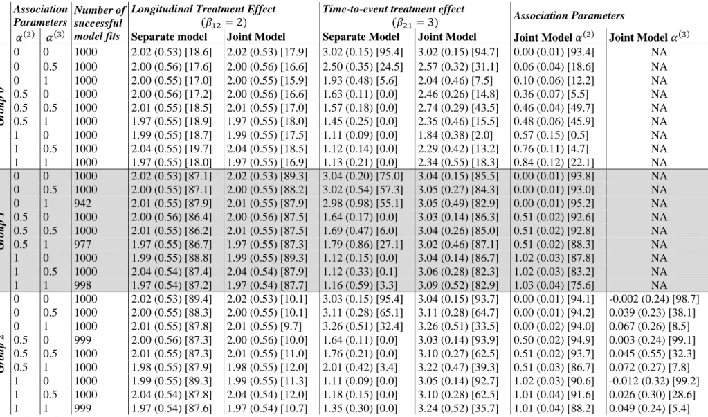
6.2.2 Results of Simulation Set 2: Differing numbers of included studies 522

The results of Simulation Set 2 are presented in Table 8. Graphical representations of the

523

mean estimates displayed in Table 8 are provided in Supplementary Figures S29-S32, with

524

representations of the point estimates from each simulation given in Supplemental Figures

525

S33-S36. The proportion of successful model fits was 99.9% or above for all model groups

526

for all scenarios investigated.

527

Longitudinal treatment effect (𝛽12) 528

Across all scenarios investigated, for both the separate and the joint analyses, the mean

529

estimate for the longitudinal treatment effect 𝛽₁₂ was close to the “true” value of 2.

530

Coverage was poor for both the separate and joint analyses for model group 0, which ignores

531

between study heterogeneity. Coverage was consistently good for the separate analyses in

532

the remaining model groups, and good for joint models from model groups 1 and 4. However

533

coverage was poor from joint models for model groups involving study level random effects.

534

Time-to-event treatment effect (𝛽21) 535

For the time-to-event treatment effect 𝛽21, we saw mean estimates from the joint analyses

536

closer to the “true” value of 3 for the joint analyses than the separate. Coverage for the

537

separate analyses was below 6% for all scenarios investigated, whilst coverage for the joint

538

models appeared best for model group 1 (above 85%), followed by model groups 4 and 5

539

(above 69%). Coverage was noticeably lower for model group 0, which ignored between

study heterogeneity, and coverage decreased for model groups 2 and 3 as the number of

541

included studies increased.

542

Association parameters (𝛼(2), 𝛼(3)) 543

The mean estimate for the individual level association was close to the “true” value of 0.5 for

544

model groups 1-5, with slightly worse estimates from model group 0. Coverage was good for

545

model groups 1, 2, 4 and 5. However coverage decreased with increasing number of studies

546

for model group 0 and 3.

547

Study level association was poorly estimates in model groups 2 and 5, with estimates closer

548

to the “true” value of 0.5 for model group 3. However coverage was consistently poor, and

549

decreased with increasing number of included studies.

550

Summary 551

Under a one-stage joint model containing a single longitudinal and single time-to-event

552

outcome, with association structure sharing both individual and study level random effects,

553

with common association parameter at each level, there appeared to be little benefit of

554

increasing number of included studies. However this result may not hold for other

555

association structures e.g. just sharing individual level random effects between studies.

556

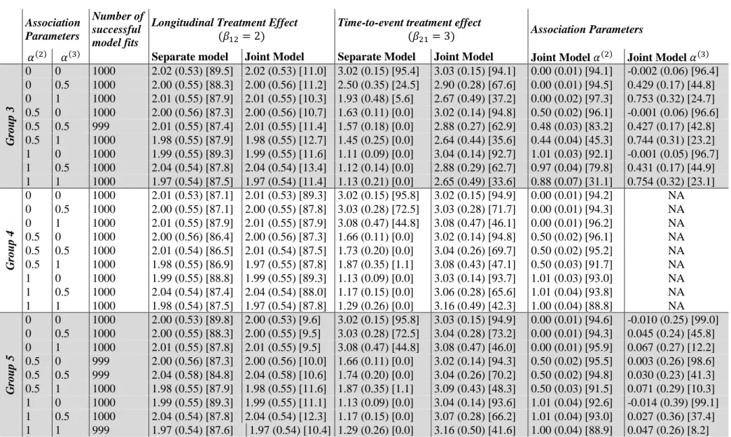
6.2.3 Results of Simulation Set 3: Differing levels of between study heterogeneity 557

The results of Simulation Set 3 are presented in Table 9. Graphical representations of the

558

mean estimates displayed in Table 9 are provided in Supplementary Figures S37-S40, with

559

representations of the point estimates from each simulation given in Supplemental Figures

560

S41-S44. There were issues with model fitting for a large proportion of simulations for model

561

groups involving study level random effects when there was no between study heterogeneity

562

(𝑨 = 𝑨_𝟏), however otherwise the proportion of successful fits was 99.8% or over.

563

Longitudinal treatment effect (𝛽12) 564

Across scenarios investigated, the mean estimated longitudinal treatment effect produced by

565

both the separate and joint one-stage MA-model were close to the “true” parameter values.

566

Coverage of estimates produced by model group 0 was good from both the separate and the

567

joint one-stage MA-models when no between study heterogeneity existed, however coverage

568

decreased as between study heterogeneity increased. For the remaining model groups,

569

coverage was consistently good for the separate analyses, but joint analyses involving study

570

level random effects displayed decreasing coverage as between study heterogeneity

571

increased.

572

Time-to-event treatment effect (𝛽21) 573

Throughout the scenarios investigated, the time-to-event treatment effect was consistently

574

underestimated by the separate analyses compared to the joint (which displayed estimates

575

closer to the “true” value of the parameters). Models involving study level random effects

576

showed estimates diverging slightly from the “true” value as between study heterogeneity

577

increased. Coverage was consistently good for model group 1, however the remaining model

578

groups displayed decreasing coverage as between study heterogeneity increased.

579

Association parameters (𝛼(2), 𝛼(3)) 580

The mean estimate for individual level association 𝛼(2) was good for model groups 1, 2, 4

581

and 5, with corresponding high coverage. However model groups 0 and 3 showed mean

582

estimates increasingly below the true value, with corresponding decreasing coverage as

583

between study heterogeneity increased.

584

Mean estimates for study level association 𝛼(3) was poor for model groups 2 and 5, and

585

closer to the true value for model group 3. Coverage was good for model groups 2 and 5 for

586

the case of no between study heterogeneity, and decreased as between study heterogeneity

587

increased. However examination of Supplemental Figure S44 indicates that wide confidence

588

intervals explained the higher coverage at no between study heterogeneity, with the width of

589

confidence intervals decreasing as between study heterogeneity increases. Coverage was

590

relatively constant but not good for model group 3 across examined levels of between study

591

heterogeneity.

592

Summary 593

Under a one-stage joint model containing a single longitudinal and single time-to-event

594

outcome, with association structure sharing both individual and study level random effects,

595

with common association parameter at each level, model group 1 appeared to be the most

596

consistently reliable modelling option. However, as noted earlier, this result may not hold for

597

other joint model specifications.

598

7 Discussion 599

In this research, we have presented and investigated a variety of models for use when

600

analysing multi-study joint longitudinal and time-to-event data. Analyses of single study

601

joint datasets are increasing8. Ensuring availability of appropriate methods for the

meta-602

analysis of such data is vital, in order to maximise use of available data and better inform

603

healthcare decisions.

604

We have examined a range of the possible modelling options, however other combinations of

605

the approaches discussed here to account for between study heterogeneity are also possible.

606

Each of the model groups examined present a range of advantages and disadvantages.

607

Models that use fixed effects to account for between study heterogeneity estimate 𝐾 − 1

608

parameters for each term involving study membership (one for each study apart from the

609

reference study). As such, results may not be generalisable to external studies, and the

610

number of parameters estimated quickly increases as the number of studies included in the

611

meta-analysis increases. However such methods do allow calculation of effect sizes within

612

each study (although this is not a primary aim of meta-analyses).

613

Conversely, use of study level random effects accounts for between study heterogeneity, but

614

study specific effect estimates are not generally automatically provided (unless the estimates

615

of the random effects can be extracted from models fitted). However this should not be an

616

issue, as meta-analyses aim to pool data rather than provide study specific estimates. The

617

number of parameters to be fitted due to study level random effects does not increase as the

618

number of included studies increases. However the distribution of the random effects may be

619

poorly estimated unless a large number of studies are included in the meta-analysis.

620

Additionally, model groups with a common baseline hazard across studies assume

621

proportional hazards across all studies included in the meta-analysis. However, model groups

622

that stratify the baseline hazard by study assume proportional hazards within but not across

623

studies. This may be a more reasonable assumption, especially if the demographics of the

624

studies differ.

The simulation investigation displayed poor performance for models that ignored any

626

between study heterogeneity present in the data. Consequently, it is clear that accounting for

627

any between study heterogeneity present in multi-study joint data is vital. The most

628

consistently well-performing model group was model group 1, which accounted for between

629

study heterogeneity using fixed study membership and interaction between study membership

630

and treatment assignment in both sub-models. The remaining model groups for the joint

631

analyses showed issues under various scenarios. As the coverage was good for separate

632

models for any model group that accounted for between study heterogeneity, the poor

633

coverage in the joint analyses for model groups 2, 3 and 5 may be due to the dual use of the

634

study level random effects to account for between study heterogeneity and account for study

635

level behaviour in the link between the longitudinal and time-to-event outcomes. It may be

636

that this dual use is not possible, unless an unrealistically large number of studies are

637

included in the meta-analysis.

638

Whilst point estimates were similar in magnitude between the separate and joint analyses for

639

the longitudinal treatment effect, we note bias in the estimates of the time-to-event treatment

640

effect from separate analyses where a non-zero association between the longitudinal and

641

time-to-event outcomes is present. This behaviour has previously been noted in single study

642

cases by Guo and Carlin18, and in two-stage joint MA analyses by Sudell et al16, our research

643

confirms that this issue persists for one-stage analyses. This behaviour may be comparable to

644

the established situation where omission of covariates from Cox models causes bias in

645

estimated effect parameters37-39_{. The 𝑊}

2𝑘𝑖(𝑡) term is included in the joint time-to-event

sub-646

model, but is not present in the separate time-to-event sub-model. Where association is

647

present (i.e. where 𝛼(2) ≠ 0 or 𝛼(3) ≠ 0), the joint analyses model risk of an event associated

648

with the longitudinal outcome through the 𝑊_2𝑘𝑖(𝑡) term. This term (which has an effect on

649

risk of an event when association is present) is not included in the separate time-to-event

650

model, giving a possible explanation for the observed biased treatment effect estimates. As

651

noted in Sudell et al16, similar behaviour was not observed between the separate and joint

652

longitudinal analyses as the model specifications for the longitudinal trajectory are identical

653

in both cases. As such, it is recommended that joint one-stage MA-models are used in place

654

of separate time-to-event one-stage MA-models where significant association exists. This

655

can be assessed prior to analyses through plotting of the longitudinal trajectories panelled by

656

event type16; differences between the trajectories between those censored and experiencing an

657

event can indicate presence of such an association.

658

The models investigated utilised an unspecified baseline hazard in the time-to-event

sub-659

model. Hseih et al40 noted that when unspecified baseline hazards are used in a joint model,

660

standard errors should be obtained through bootstrapping procedures to avoid their

661

underestimation. As such, the time commitment to perform bootstrapping procedures on

662

large meta-datasets was considerable. Performing bootstrapping procedures on a standard

663

computing environment took several days for the real dataset. Consequently bootstraps were

664

performed in parallel using the University of Liverpool’s HTCondorsystem (see41,

665

https://research.cs.wisc.edu/htcondor/, and http://condor.liv.ac.uk/ which was also used to run

666

the simulations), with the results compiled using purpose written code rather than relying on

667

single computer bootstrapping procedures. Researchers using large datasets without coding

668

experience or access to such computer systems may experience issues conducting large scale

669

joint data meta-analyses.

670

In our clinical example, we assume common association parameters across treatment groups.

671

However, in reality, the association between the longitudinal blood pressure and risk of an

672

event could differ between those assigned to any treatment for hypertension versus those

assigned to placebo, no treatment or usual care42. In single study cases, association structures

674

involving interactions between baseline covariates and the association parameters have been

675

presented2,4_{, however this association structure has not yet been investigated in meta-analytic} 676

joint models.

677

The research presented here prompts a range of future areas of research. Investigation of

678

one-stage joint MA-models with varying association structures, including sharing only

679

individual level random effects or sharing the current value of the longitudinal trajectory, is

680

vital. Additionally, it is vital to investigate alternative modelling options, such as alternative

681

baseline hazard specifications, with could reduce model fitting times by removing the

682

necessity of bootstrapping. Also, in our simulation study, we assumed common longitudinal

683

measurement schedules across the included studies, identical numbers of individuals

684

recruited to each study, and common association parameter across studies. Further

685

simulation investigations varying these aspects could provide additional useful information

686

for future joint data meta-analyses.

687

In conclusion, this research indicates the benefit of the one-stage meta-analysis of joint

688

longitudinal and time-to-event data where significant association exists between the

689

longitudinal and time-to-event outcomes. Given the current research, it is recommended that

690

analyses do not rely on models that share study level random effects between sub-models.

691

Further research into one-stage joint MA-models is required.

692

Acknowledgements 693

We would like to thank the INDANA collaboration26, for use of the dataset for the real data

694

analysis, as well as the individual studies contained in this dataset27-32,43. This work was

695

supported by the Health eResearch Centre (HeRC) funded by the Medical Research Council

696

Grant MR/K006665/1.

697

References 698

1. Wulfsohn MS, Tsiatis AA. A Joint Model for Survival and Longitudinal Data Measured with 699

Error. International Biometric Society. 1997(1):330. 700

2. Gould AL, Boye ME, Crowther MJ, et al. Joint modeling of survival and longitudinal non-701

survival data: current methods and issues. Report of the DIA Bayesian joint modeling 702

working group. Stat Med. Jun 30 2015;34(14):2181-2195. 703

3. Henderson R, Diggle P, Dobson A. Joint modelling of longitudinal measurements and event 704

time data. Biostatistics (Oxford, England). 2000;1(4):465-480. 705

4. Rizopoulos D. Joint Models for Longitudinal and Time-to-Event Data With Applications in R.

706

Vol 1. 1 ed2012. 707

5. Tsiatis AA, Davidian M. Joint modeling of longitudinal and time-to-event data: An overview. 708

STATISTICA SINICA. 2004;14(3):809-834. 7