SUBSPECTRALNET – USING SUB-SPECTROGRAM BASED CONVOLUTIONAL NEURAL
NETWORKS FOR ACOUSTIC SCENE CLASSIFICATION
Sai Samarth R Phaye
1, Emmanouil Benetos
2,3, and Ye Wang
11
School of Computing, National University of Singapore, Singapore
2
School of EECS, Queen Mary University of London, UK
3The Alan Turing Institute, UK
ABSTRACT
Acoustic Scene Classification (ASC) is one of the core research problems in the field of Computational Sound Scene Analysis. In this work, we present SubSpectralNet, a novel model which cap-tures discriminative feacap-tures by incorporating frequency band-level differences to model soundscapes. Using mel-spectrograms, we pro-pose the idea of using band-wise crops of the input time-frequency representations and train a convolutional neural network (CNN) on the same. We also propose a modification in the training method for more efficient learning of the CNN models. We first give a motivation for using sub-spectrograms by giving intuitive and statis-tical analyses and finally we develop a sub-spectrogram based CNN architecture for ASC. The system is evaluated on the public ASC development dataset provided for the “Detection and Classification of Acoustic Scenes and Events” (DCASE) 2018 Challenge. Our best model achieves an improvement of +14% in terms of classification accuracy with respect to the DCASE 2018 baseline system. Code and figures are available athttps://github.com/ssrp/SubSpectralNet
Index Terms— Acoustic Scene Classification, Convolutional Neural Networks, Computational Sound Scene Analysis.
1. INTRODUCTION
The problem of recognizing the acoustic soundscapes and identify-ing the environment in which a sound is recorded is known as Acous-tic Scene Classification [1, 2]. The objective is to assign a semanAcous-tic label (acoustic scene) to the input audio stream that characterizes the type of environment in which it is recorded – for example shopping mall, airport, street. The problem has been very well explored as a single-label classification task [3, 4]. Due to the possible presence of diverse sound events in a sound scene, developing a descriptive representation for ASC is known to be a difficult task [5].
DCASE Challenges, started in 2013, provide benchmark data for computational sound scene analysis research, including tasks for detection and classification of acoustic scenes and events, motivat-ing researchers to further work in this area. Lookmotivat-ing at the current trend of challenge submissions in the ASC task, it is clear that re-searchers are moving towards using deep learning methods for sys-tem development [3, 4, 6]. This is because of the fact that the cur-rent hand-crafted methods are not sufficient to capture the discerning properties of soundscapes [7]. With time, data-driven approaches are taking over conventional methods which involve more expert knowl-edge for designing and choosing features. Most published systems typically use a combination of audio descriptors and learning tech-niques, with a growing inclination towards deep learning [8, 9].
EB is supported by RAEng Research Fellowship RF/128 and EPSRC Grant EP/R01891X/1. This work was supported by The Alan Turing Institute under the EPSRC grant EP/N510129/1.
The literature of ASC research is vast and a lot has been done in system design. Earliest works in this field have tried to use numer-ous methods from speech recognition (for example, using features like Mel-frequency cepstral coefficients [10], normalized spectral features, and low-level features [2, 11] like the zero-crossing rate). General architecture follows a pipeline based on extracting frame-by-frame hand-crafted audio features or learning them using various methods like matrix decomposition of spectral representations (log mel-spectrograms [12], Constant-Q transformed spectrograms [13]), and then performing machine learning based classification. The fi-nal decision is a combination of frame wise outputs, for example, by using majority voting or mean probability. Many systems incor-porate deep learning approaches, generally by using some kind of time-frequency representation as the input and training deep neural networks (DNNs) or CNNs [14, 15]. Some methods also exploited ideas from the image processing literature, for example, training a classifier using the histogram of gradient representations over spec-trograms of audio frames [16, 17].
CNNs are extensively used in ASC. Some systems incorporate the use of convolutional layers with large receptive fields (kernels) to capture global correlations in the spectrograms [18, 19], while some use smaller kernels focusing on local spatial data [20, 14]. Rather than aiming for state of the art results, our goal is to show how sub-spectrograms could be used in CNNs to infer sound scenes more efficiently. Our work shows that depending on the scene class, there is a specific frequency band showing most activity, hence providing discriminative features for that class; to the authors’ knowledge this has not been considered in earlier studies. We first develop a motiva-tion for using spectrogram crops, which we termSub-spectrograms. Finally, we propose a CNN model,SubSpectralNet, to make use of the Sub-spectrograms to capture more enhanced features, hence re-sulting in superior performance over a model with similar parameters which does not incorporate sub-spectrograms (discussed in Section 4). For all experiments, we used the DCASE 2018 ASC development dataset [21] having 6122 two-channel 10-second samples for train-ing and 2518 samples for testtrain-ing, divided into ten acoustic scenes.
The rest of the paper is divided as follows – in Section 2, we develop a basic statistical model for ASC which we use as the moti-vation to design the proposed CNN architecture. Section 3 discusses the methodology used to develop the CNN model and Section 4 de-scribes various experiments performed to prove the efficacy of the system. Finally, we conclude the work in Section 5.
2. STATISTICAL ANALYSIS OF SPECTROGRAMS
Magnitude spectrograms are two-dimensional representations over time and frequency, which are very different from real life images. In spectrograms, there is a clear variation in the frequency axis. While
0 25 50 75 100 125 150 175 200
Mel-bins (low to high)
0.0 0.2 0.4 0.6 0.8 1.0 Activation
Class: airport
(a) 0 25 50 75 100 125 150 175 200Mel-bins (low to high)
0.0 0.2 0.4 0.6 0.8 1.0 Activation
Class: bus
(b) 0 25 50 75 100 125 150 175 200Mel-bins (low to high)
0.0 0.2 0.4 0.6 0.8 1.0 Activation
Class: metro
(c) 0 25 50 75 100 125 150 175 200Mel-bins (low to high)
0.0 0.2 0.4 0.6 0.8 1.0 Activation
Class: street_traffic
(d) 0 25 50 75 100 125 150 175 200Mel-bins (low to high)
0.0 0.2 0.4 0.6 0.8 1.0 Activation
Class: tram
(e) 0 25 50 75 100 125 150 175 200Mel-bins (low to high)
0.0 0.2 0.4 0.6 0.8 1.0 Activation
Class: park
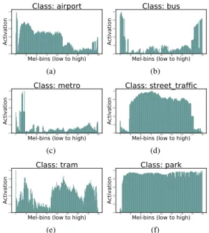
(f)Fig. 1: Histogram of activation of mel-bins for some sound scene
classes. We can infer the importance of specific mel-bins for spe-cific classes from these histograms. This is also intuitively true, for example, in an airport or in a metro, audio may have dominant and discriminative low-frequency noise, and lower bands of the spectro-grams show more activation for these classes.
images have local relationships over both spatial dimensions, spec-trograms have definitive local relationships in the time dimension, but not in the frequency dimension. In the frequency dimension, for some types of sounds there are local relationships (e.g. sounds that have broadband spectra like noise-like sounds), sometimes they have non-local relationships (e.g. harmonic sounds, where there are relationships between non-adjacent frequency bins), and sometimes there are simply no local relationships at all.
We first create a simple mathematical model to gain more in-sights on how CNNs could leverage time-frequency features effi-ciently. We extract log mel-spectrograms using a 2048-point short time Fourier transform (STFT) on 40ms Hamming windowed frames with 20ms overlap and then transform this into 200 Mel-scale band energies. Finally, the log of these energies is taken. Next, we per-form bin-wise normalization of the sample space and obtain 6122 samples having200×500(mel-bins×time-index) feature size. Now, we concatenate all the samples of the same class in the time di-mension and take the average of the temporal direction to obtain ten distributions having 200 vector-size, one for each class. We observe that there is a clear variation in the class-wise activation of different mel-bins. For more clarity, we perform bin-wise classification of test samples using the ten 200D reference mean vectors.
For each test sample, we compute the mean of temporal direc-tion to get a 200D vector and the hypothesis is that this vector should have a similar distribution as that for the mean vector of the corre-sponding class. Mathematically, we compute the L2 distance with the reference mean vectors and the class for which this distance has the minimum value should be the correct label.
Now, instead of computing the distance measure for the whole 200D vector, we compute separate distances for each mel-bin be-cause we are interested in analyzing how those bins are activated
airport busmetro metro_station
park
public_squareshopping_mallstt_pedestrianstreet_traffic tram airport bus metro metro_station park public_square shopping_mall stt_pedestrian street_traffic tram 1 0.028 0.048 0.108 0.005 0.027 0.202 0.067 0.02 0.076 0.028 1 0.181 0.237 0 0.016 0.045 0.165 0 0.031 0.048 0.181 1 0.246 0 0.014 0.082 0.192 0 0.024 0.108 0.237 0.246 1 0 0.028 0.09 0.22 0.001 0.032 0.005 0 0 0 1 0.017 0.007 0.001 0.088 0.025 0.027 0.016 0.014 0.028 0.017 1 0.124 0.131 0.032 0.075 0.202 0.045 0.082 0.09 0.007 0.124 1 0.228 0.017 0.148 0.067 0.165 0.192 0.22 0.001 0.131 0.228 1 0.006 0.154 0.02 0 0 0.001 0.088 0.032 0.017 0.006 1 0.026 0.076 0.031 0.024 0.032 0.025 0.075 0.148 0.154 0.026 1
Fig. 2: Resultant Chi-Square Distance Matrix.
for specific classes. This is equivalent to saying that we have 200 small classifiers. Finally, using these 200 outputs for all the test sam-ples, we create one normalized histogram for each class, in which we have frequencies of correct classifications of corresponding mel-bins, shown in Fig. 1. We also calculate the chi-square distance be-tween these histograms to see how similar class-wise distributions are. For this, we normalize the histograms with maximum value to one, and then compute the distance. The lesser the distance, the more confusion exists between those classes. We aim to obtain a matrix which has some resemblance with a confusion matrix. For that, after getting the10×10symmetrical matrix having distances between the classes, we normalize the matrix by dividing with the maximum value. Then, we apply the following mathematical transform:
xnewij = 1−e
−kxij (1)
wherexijis the prior distance value andi, jare the matrix indices. kis a constant parameter which when increased, enhances the dif-ferences of values on the higher range. We usedk as10so that the matrix resembles a confusion matrix. Next, we normalize again the matrix by dividing with the maximum value and lastly, subtract these values from one. The output of this is shown in Fig. 2. We also compute the Kullback-Leibler divergence [22] and Hellinger distance [23] over these histograms and they result in a very simi-lar matrix, which shows that the statistical model is robust. We can clearly see that some classes are having higher confusions (for
exam-ple,“metro station”and“metro”;“shopping mall”and“airport”),
which resembles the confusion matrices obtained from the baseline model results [21] and proposed CNN model (shown in Figure 4).
In the histograms obtained, we observe a definite variation of ac-tivation of mel-bins and sub-bands, which is specific to every scene. For example, the“metro”class has more activation in lower fre-quency bins; the“bus”has less activation in mid frequency bins. For
“park”or“street traffic”, nearly all mel-bins are active and from
the DCASE 2018 baseline result [21], we can see that these classes have relatively superior performance. We use these observations to develop SubSpectralNet, which is discussed in the next section.
3. DESIGNING SUBSPECTRALNET
We start off with the DCASE 2018 baseline system for the ASC task and gradually develop the proposed network. The baseline system is based on a CNN, where mel-band energies with 40 mel-bins are extracted for every sample with 40 millisecond frame size and 50% overlap using 2048-point STFT. The samples are further normalized and the size of each sample is40×500. These samples are passed
to a CNN consisting of two layers withsamepadding in order – 32 kernels and 64 kernels, each having kernels of7×7size, batch normalization and ReLU activation. After each conv-layer, a max-pooling layer of5×5and4×100pool-size respectively is used to decrease the size of the feature space and a dropout rate of 30% is applied to prevent over-fitting. Finally, a fully connected (FC) layer with 100 neurons is used over the flattened output, which is further connected to the output (softmax) layer.
We train DCASE 2018 baseline models on different channels of the audio dataset – left channel, right channel, average-mono chan-nel and lastly, both chanchan-nels to the CNN model. The best results are obtained using both channels which is expected as binaural in-put would give more information on the prominent sound events in soundscapes, for example, a car passing by in“street traffic”.
3.1. Incorporating Sub-spectrograms
From the analysis in Section 2, we infer that using bigger convolu-tional kernels over spectrograms is not a good idea because it tends to combine global context and we lose the local time-frequency infor-mation. We perform an experiment (discussed in Section 4) in which we gradually increase the size of the kernels in the first conv-layer of the baseline system. The accuracy decreases with the increase in kernel size. Spectrograms have a definite variation in the frequency dimension. Using smaller convolutional kernels over complete spec-trograms works fine because CNNs are very powerful in fitting these receptive fields to understand the variances in the data. But the fact that spectrograms have these variations could be advantageous.
Building upon this idea, we propose SubSpectralNet and its ar-chitecture is shown in Figure 3. SubSpectralNet essentially creates horizontal slices of the spectrogram and trains separate CNNs on these sub-spectrograms, finally acquiring band-level relations in the spectrograms to classify the input using diversified information.
We extract the log mel-energy spectrograms for theNsamples and perform bin-wise normalization. For creating sub-spectrograms, we design a new layer (we term it asSubSpectral Layer) which splits the spectrogram into various horizontal crops. It takes three inputs – input spectrogram (C×F ×T dimension,C, F andT being number of channels, mel-bins and time-indices respectively), sub-spectrogram sizeX and mel-bin hop-size (vertical hop)Y. This results inM frequency-time sub-spectrograms ofC×X×T di-mension for every sample, whereM =b1 + (F−X)/Yc.
3.2. SubSpectralNet – Architecture Details
Two-channel sub-spectrograms are independently connected to 2 conv-layers withsamepadding and kernel-size of(7,7)having 32 and 64 kernels respectively. After each conv-layer, there is a batch normalization layer, ReLU activation layer, max-pooling layers of
(X/10,5)and (4,100)size respectively, and finally a dropout of 30%. After the second pooling, we flatten the layer and add an FC layer with 32 neurons with ReLU activation and 30% dropout, followed by the softmax layer. We call these sub-classifiers of the SubSpectralNet. We do not remove these softmax outputs from the final network because this enforces them to learn to classify the sample based on only a part of spectrogram. We keep most param-eters same as the DCASE 2018 baseline model for fair comparison. We believe that sub-spectrograms could be incorporated into more complex architectures [24, 25, 26] that could be used to surpass the state of the art in ASC performance.
To capture the global correlation (or de-correlation) between frequency bands, we concatenate the FC (ReLU) layer of the
sub-. sub-. sub-. Sub-CNN 2 . . . . . . . . . Sub-Classifier Output 1 Sub-CNN 1 Sub-CNN M Global Classifier Sub-Classifier Output 2 Sub-Classifier Output M FC 1 Layer FC 2 Layer FC H Layer 2 × F × T Spectrogram Input Conv-Layer 1 (32 × X × T) BN, ReLU MP(X/10, 5), Dropout(0.3) Concat BN, ReLU, MP(4,100), Dropout(0.3) Flatten, FC(32), Dropout(0.3) T X Y Conv-Layer 2 (64 × 10 × T/5) SubSpectral Layer BN: BatchNorm MP: MaxPool FC: Fully Connected Layer Conv Kernels: (7 × 7)
Global Classification Sub-network
...
. . .
Fig. 3: Proposed pipeline of SubSpectralNet.
networks and train a DNN withH hidden layers withRineurons, where:H =max(blog2(M)c −1,0);Ri= 26+H−i,1≤i≤H. We term this as theglobal classification sub-network.
All cross-entropy errors from the global and sub-classifiers are back-propagated simultaneously to train a single network. The sub-classifiers learn to classify using specific bands of spectrograms, while the global classifier combines and learns discerning informa-tion at the global level. This modificainforma-tion of training method results in improved performance and faster convergence of the model with minimal addition to the complexity [24].
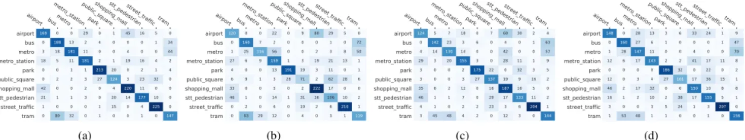
We create confusion matrices (shown in Fig. 4) from the output of these sub-classifiers and the global classification model discussed in Section 4. We observe that the statistical motivation given in Sec-tion 2 fits well with the results. For example, for the“airport”class, statistical distribution says that lower frequencies are more effective in classification. The same is shown in the confusion matrix where the low-band sub-classifier shows better results for this class. For
the“bus”class, the mid-band sub-classifier shows relatively better
results. For most classes, the global classifier achieves better results than any sub-classifier. It is interesting to note that for some classes
like“public square”or“tram”, a sub-classifier performs better than
the global classifier, which could mean that using the complete trogram adds outliers and it is better to use a specific band of spec-trogram in such case.
4. EXPERIMENTS
We demonstrate the potential of SubSpectralNet on the DCASE 2018 development public dataset (Task 1A) and compare the results with DCASE 2018 baseline. We use dcase util toolbox [27] to the extract features from the DCASE 2018 dataset. We implement SubSpectralNet in Keras with TensorFlow backend and experiments are performed on an NVIDIA Titan Xp GPU having 12GB RAM. We train all models 3 times for 200 epochs and report the average-best accuracy. The learning rate is set to0.001with Adam as the optimizer. Following are the experiments we perform in this work:
We train DCASE 2018 baseline models on different channels of audio dataset and the test accuracy achieved are 63.24% (left chan-nel), 61.83% (right chanchan-nel), 64.91% (average-mono channel) and
65.66%(stereo channels). We also train the DCASE 2018
base-line model for various kernel sizes of the first CNN layer –(7,7),
(15,15),(25,25)and(35,35). The corresponding test accuracies
are65.66%, 65.23%, 65.08% and 62.80% respectively. This shows
airport busmetro metro_station
park
public_squareshopping_mallstt_pedestrianstreet_traffic tram airport bus metro metro_station park public_square shopping_mall stt_pedestrian street_traffic tram 169 0 0 29 0 1 45 16 5 0 0 188 13 2 4 0 0 0 1 34 3 18 181 11 0 0 4 0 0 44 18 5 11 181 2 1 19 16 4 2 0 0 1 1 213 20 0 2 1 4 0 2 2 3 27 124 3 23 32 0 42 0 0 2 0 4 220 11 0 0 21 1 1 3 0 20 14 177 10 0 1 0 0 0 1 15 0 4 225 0 0 80 32 0 1 0 0 1 0 147 (a) airport busmetro metro_station park
public_squareshopping_mallstt_pedestrianstreet_traffic tram airport bus metro metro_station park public_square shopping_mall stt_pedestrian street_traffic tram 120 0 0 22 0 9 80 29 5 0 0 160 7 2 0 0 0 1 0 72 1 25 116 56 0 0 2 3 8 50 27 6 9 159 1 3 19 21 13 1 4 0 0 13 191 19 3 11 0 1 6 9 1 3 28 71 2 62 28 6 33 0 0 5 0 2 222 17 0 0 46 1 0 14 1 31 36 106 10 2 0 2 0 6 0 19 2 6 210 1 0 93 29 12 0 4 0 3 1 119 (b) airport busmetro metro_station park
public_squareshopping_mallstt_pedestrianstreet_traffic tram airport bus metro metro_station park public_square shopping_mall stt_pedestrian street_traffic tram 124 5 7 18 0 7 68 30 2 4 0 142 23 3 6 0 4 0 1 63 4 14 130 14 0 0 42 0 0 57 29 3 20 155 3 0 28 11 1 9 3 0 0 2 175 22 0 32 3 5 3 0 0 3 27 137 19 9 16 2 35 6 2 12 0 16 187 16 5 0 46 1 1 7 0 29 17 133 11 2 4 1 0 2 2 23 3 6 204 1 3 45 48 4 2 0 12 3 0 144 (c) airport busmetro metro_station park
public_squareshopping_mallstt_pedestrianstreet_traffic tram airport bus metro metro_station park public_square shopping_mall stt_pedestrian street_traffic tram 148 0 28 13 3 6 33 24 1 9 0 160 27 6 1 0 0 0 1 47 1 28 147 11 0 0 4 0 0 70 12 6 17 143 2 2 41 17 11 8 0 0 0 0 186 32 0 22 0 2 12 0 3 4 27 101 17 36 15 1 46 2 17 32 0 6 150 10 8 8 16 1 2 10 2 38 17 155 5 1 3 0 0 3 5 24 1 3 207 0 1 53 48 1 1 0 0 1 0 156 (d)
Fig. 4: Confusion matrices obtained from a SubSpectralNet trained over 40 mel-bin spectrograms, 20 sub-spectrogram size, 10 mel-bin
hop-size, hence 3 sub-classifiers and one global classifier. Matrices are obtained for (a) Global Classifier, (b) High-frequency Band Sub-Classifier (21-40 mel-bins), (c) Mid-frequency Band Sub-Classifier (11-30 mel-bins) and (d) Low-frequency Band Sub-Classifier (1-20 mel-bins).
0 25 50 75 100 125 150 175 200 Training Epoch 40 45 50 55 60 65 70
Test Accuracy Global ClassifierHigh-Freq Sub-classifierMid-Freq Sub-classifier Low-Freq Sub-classifier Baseline Results
Fig. 5: Comparison of performance between the multi-channel
DCASE 2018 baseline model and SubSpectralNet on 40 mel-bin spectrograms, 20 sub-spectrogram size and 10 mel-bin hop-size.
scale, hence losing local spatial information. As a result, we choose the kernel-size of(7,7)with stereo input for SubSpectralNet.
We train a SubSpectralNet model on 40 log mel-energy spectro-grams with 20 sub-spectrogram size and 10 mel-bin hop-size (331K model parameters). The resultant accuracy we achieve from this is
72.18%. The confusion matrices computed for this model are shown
in the Figure 4. Also, we plot a curve of training epoch versus test accuracy, comparing the performance of the DCASE 2018 baseline (2-channel model) and this SubSpectralNet model, which is shown in Figure 5. It can be seen that SubSpectralNet (global classifier) has a relatively faster convergence with superior test accuracy.
To demonstrate the importance of sub-classifiers, we train a SubSpectralNet model excluding the Sub-Classifier (softmax lay-ers) back-propagations and only use the global classification sub-network (330K model parameters). This achieves an accuracy of 68.79%, comparing to 72.18% with the sub-classifiers, which ver-ifies the significance of the same. More experiments with 40 log mel-energy spectrograms are shown in Figure 6 (a).
Parameters of a CNN are one of the major criteria to compare two models. The DCASE 2018 baseline model on 40 mel-bins has 117K parameters (using 2-channel input) and the SubSpectralNet model with 20 sub-spectrogram size and 10 mel-bin hop-size has 331K parameters. To prove the efficacy of SubSpectralNet, we mod-ified the DCASE 2018 baseline model by doubling the number of kernels in both conv-layers (now 64 and 128). This model, having 434K parameters achieved 66.79% accuracy which is5.39%lower than the accuracy of proposed model. Hence, this justifies the fact that the idea of fitting separate kernels (training separate CNNs) over separate bands of spectrograms learns more salient features than di-rectly training a CNN on spectrograms.
10 20 30 Sub-Spectrogram Size 66 68 70 72 74 Test Accuracy 70.56 72.18 67.32 (a) 10 20 30 40 50 60 Sub-Spectrogram Size 71 72 73 74 75 Test Accuracy 71.94 74.03 74.08 72.75 73.31 72.67 (b) (20, 10) (40, 20) (80, 40) (Sub-Spectrogram Size, Mel-bin Hop)71
72 73 74 75 Test Accuracy 74.03 73.45 72.03 (c)
Fig. 6: Results obtained by SubSpectralNet on – (a) 40 mel-bin
spectrogram and 10 mel-bin hop-size; (b) 200 mel-bin spectrogram with 10 mel-bin hop-size; (c) 200 mel-bin spectrogram, varying sub-spectrogram and mel-bin hop-size.
Considering that 200 mel-bin spectrograms achieve better per-formance than using lesser mel-bins [19], we train a DCASE 2018 baseline model on 200 mel-bins and the accuracy achieved is 71.94%. It is interesting to note that SubSpectralNet with 40 mel-bins can achieve comparably superior accuracy. We trained various SubSpectralNets on 200 mel-bins and the results are shown in Fig. 6 (b) and (c). The best accuracy achieved was 74.08%, by using 30 sub-spectrogram size and 10 mel-bin hop-size, which is an overall increase of+14%over the DCASE 2018 baseline [21].
5. CONCLUSIONS
In this paper, we introduce a novel approach of using spectrograms in Convolutional Neural Networks in the context of acoustic scene classification. First, we show from the statistical analysis of Sec. 2 that some specific bands of mel-spectrograms carry more discrimina-tive information than other bands, which is specific to every sound-scape. From the inferences taken by this, we propose SubSpectral-Nets in which we first design a new convolutional layer that splits the time-frequency features into sub-spectrograms, then merges the band-level features on a later stage for the global classification. The effectiveness of SubSpectralNet is demonstrated by a relative im-provement of +14% accuracy over the DCASE 2018 baseline model. SubSpectralNets also have some limitations, including the fact that for some classes, sub-classifiers perform better than the global classifier. Also in the current model, we have to specify parame-ters like sub-spectrogram size and mel-bin hop-size. One way to address this could be by using the statistical analysis to choose the most appropriate parameters. In future, we plan to work on further improving the performance of this network, for example, by incor-porating well-founded CNN architectures [25, 26] or modelling the temporal information of SubSpectralNets in a more effective way.
6. REFERENCES
[1] Tuomas Virtanen, Mark D Plumbley, and Dan Ellis,
Computa-tional analysis of sound scenes and events, Springer, 2018.
[2] Antti J Eronen, Vesa T Peltonen, Juha T Tuomi, Anssi P Kla-puri, Seppo Fagerlund, Timo Sorsa, Ga¨etan Lorho, and Jyri Huopaniemi, “Audio-based context recognition,”IEEE
Trans-actions on Audio, Speech, and Language Processing, vol. 14,
no. 1, pp. 321–329, 2006.
[3] Dan Stowell, Dimitrios Giannoulis, Emmanouil Benetos, Mathieu Lagrange, and Mark D Plumbley, “Detection and clas-sification of acoustic scenes and events,”IEEE Transactions on
Multimedia, vol. 17, no. 10, pp. 1733–1746, 2015.
[4] Annamaria Mesaros, Toni Heittola, Emmanouil Benetos, Pe-ter FosPe-ter, Mathieu Lagrange, Tuomas Virtanen, and Mark D Plumbley, “Detection and classification of acoustic scenes and events: Outcome of the DCASE 2016 challenge,”IEEE/ACM Transactions on Audio, Speech and Language Processing
(TASLP), vol. 26, no. 2, pp. 379–393, 2018.
[5] Yifang Yin, Rajiv Ratn Shah, and Roger Zimmermann, “Learning and fusing multimodal deep features for acoustic scene categorization,” in2018 ACM Multimedia Conference
on Multimedia Conference. ACM, 2018, pp. 1892–1900.
[6] Tuomas Virtanen, Annamaria Mesaros, Toni Heittola, Alek-sandr Diment, Emmanuel Vincent, Emmanouil Benetos, and Benjamin Martinez Elizalde,Proceedings of the Detection and Classification of Acoustic Scenes and Events 2017 Workshop
(DCASE2017), Tampere University of Technology. Laboratory
of Signal Processing, 2017.
[7] Mathieu Lagrange, Gr´egoire Lafay, Boris Defreville, and Jean-Julien Aucouturier, “The bag-of-frames approach: a not so sufficient model for urban soundscapes,” The Journal of the
Acoustical Society of America, vol. 138, no. 5, pp. EL487–
EL492, 2015.
[8] Victor Bisot, Romain Serizel, Slim Essid, and Ga¨el Richard, “Feature learning with matrix factorization applied to acous-tic scene classification,” IEEE/ACM Transactions on Audio,
Speech, and Language Processing, vol. 25, no. 6, pp. 1216–
1229, 2017.
[9] Huy Phan, Lars Hertel, Marco Maass, Philipp Koch, and Al-fred Mertins, “Label tree embeddings for acoustic scene clas-sification,” inProceedings of the 2016 ACM on Multimedia
Conference. ACM, 2016, pp. 486–490.
[10] Jean-Julien Aucouturier, Boris Defreville, and Francois Pachet, “The bag-of-frames approach to audio pattern recognition: A sufficient model for urban soundscapes but not for polyphonic music,”The Journal of the Acoustical Society of America, vol. 122, no. 2, pp. 881–891, 2007.
[11] Jurgen T Geiger, Bjorn Schuller, and Gerhard Rigoll, “Large-scale audio feature extraction and svm for acoustic scene clas-sification,” inApplications of Signal Processing to Audio and
Acoustics (WASPAA), 2013 IEEE Workshop on. IEEE, 2013,
pp. 1–4.
[12] Benjamin Cauchi, Mathieu Lagrange, Nicolas Misdariis, and Arshia Cont, “Saliency-based modeling of acoustic scenes us-ing sparse non-negative matrix factorization,” inImage Anal-ysis for Multimedia Interactive Services (WIAMIS), 2013 14th
International Workshop on. IEEE, 2013, pp. 1–4.
[13] Victor Bisot, Romain Serizel, Slim Essid, and Ga¨el Richard, “Acoustic scene classification with matrix factorization for un-supervised feature learning,” inAcoustics, Speech and Signal
Processing (ICASSP), 2016 IEEE International Conference on.
IEEE, 2016, pp. 6445–6449.
[14] Michele Valenti, Aleksandr Diment, Giambattista Parascan-dolo, Stefano Squartini, and Tuomas Virtanen, “DCASE 2016 acoustic scene classification using convolutional neural net-works,” IEEE AASP Challenge on Detection and Classifica-tion of Acoustic Scenes and Events (DCASE2016), Budapest,
Hungary, 2016.
[15] Karol J Piczak, “Environmental sound classification with con-volutional neural networks,” inMachine Learning for Signal Processing (MLSP), 2015 IEEE 25th International Workshop on. IEEE, 2015, pp. 1–6.
[16] Victor Bisot, Slim Essid, and Ga¨el Richard, “Hog and subband power distribution image features for acoustic scene classifica-tion,” inSignal Processing Conference (EUSIPCO), 2015 23rd
European. IEEE, 2015, pp. 719–723.
[17] Alain Rakotomamonjy and Gilles Gasso, “Histogram of gradi-ents of time-frequency representations for audio scene classifi-cation,” IEEE/ACM Transactions on Audio, Speech and
Lan-guage Processing (TASLP), vol. 23, no. 1, pp. 142–153, 2015.
[18] Karol J Piczak, “Environmental sound classification with con-volutional neural networks,” inMachine Learning for Signal Processing (MLSP), 2015 IEEE 25th International Workshop on. IEEE, 2015, pp. 1–6.
[19] Karol J Piczak, “The details that matter: Frequency resolution of spectrograms in acoustic scene classification,” Detection
and Classification of Acoustic Scenes and Events, 2017.
[20] Yoonchang Han, Jeongsoo Park, and Kyogu Lee, “Con-volutional neural networks with binaural representations and background subtraction for acoustic scene classification,” the Detection and Classification of Acoustic Scenes and Events
(DCASE), pp. 1–5, 2017.
[21] Annamaria Mesaros, Toni Heittola, and Tuomas Virtanen, “A multi-device dataset for urban acoustic scene classification,”
inProceedings of the Detection and Classification of Acoustic
Scenes and Events 2018 Workshop (DCASE2018), November
2018, pp. 9–13.
[22] Solomon Kullback and Richard A Leibler, “On information and sufficiency,” The annals of mathematical statistics, vol. 22, no. 1, pp. 79–86, 1951.
[23] Rudolf Beran et al., “Minimum hellinger distance estimates for parametric models,” The annals of Statistics, vol. 5, no. 3, pp. 445–463, 1977.
[24] Sai Samarth R Phaye, Apoorva Sikka, Abhinav Dhall, and Deepti Bathula, “Multi-level dense capsule networks,” inProc.
of the Asian Conference on Computer Vision (ACCV), 2018.
[25] Jie Hu, Li Shen, and Gang Sun, “Squeeze-and-excitation net-works,” inIEEE Conference on Computer Vision and Pattern
Recognition (CVPR), 2018, pp. 7132–7141.
[26] Gao Huang, Zhuang Liu, Laurens Van Der Maaten, and Kil-ian Q Weinberger, “Densely connected convolutional net-works,” inIEEE Conference on Computer Vision and Pattern
Recognition (CVPR), 2017, pp. 2261–2269.
[27] Toni Heittola, “DCASE UTIL: utilities for detection and classification of acoustic scenes,” 2018, https://dcase-repo.github.io/dcase util/index.html.