APPROXIMATION OF PERIODIC FUNCTIONS
MOHSIN JAVED∗‡ AND LLOYD N. TREFETHEN† ‡
Abstract. In this paper we present an implementation of the Remez algorithm for trigonometric minimax approximation of periodic functions. There are software packages which implement the Remez algorithm for even periodic functions. However, we believe that this paper describes the first implementation for the general periodic case. Our algorithm uses Chebfun to compute with periodic functions. For each iteration of the Remez algorithm, to construct the approximation, we use the second kind barycentric trigonometric interpolation formula instead of the first kind formula. To locate the maximum of the absolute error, instead of dense sampling of the error function, we use Chebfun’s eigenvalue based root finding method applied to the Chebyshev representation of the derivative of the underlying periodic function. Our algorithm has applications for designing FIR filters with real but asymmetric frequency responses.
Key words. Remez, Chebfun, trigonometric interpolation, best approximation, periodic func-tions, barycentric formula, root finding
AMS subject classifications. 41A50, 42A10, 42A15, 65T40
1. Introduction. The paper focusses on the classical problem of finding the minimax approximation of a real-valued periodic function in the space of trigonometric polynomials. The well known Remez algorithm is a nonlinear iterative procedure for finding minimax approximations. It is more than 80 years old and an account of its historical development can be found in [10], which focusses on the familiar case of approximation by algebraic polynomials. As we shall see, after some variations, the same algorithm can be used to approximate continuous periodic functions by trigonometric polynomials.
After the advent of digital computers, the Remez algorithm became popular in the 1970s due to its applications in digital filter design [11]. Since the desired filter response is typically an even periodic function of the frequency, the last 40 years have seen a sustained interest in finding the minimax approximation of even periodic func-tions in the space of cosine polynomials. This design problem, as shown in [11], after a simple change of variables, reduces to the problem of finding minimax approxima-tions in the space of ordinary algebraic polynomials. There is a good deal of literature concerning such approximations, but very little which deals with the general periodic case. What literature there is appears not to solve the general best approximation problem but only certain variations of it as used in digital filtering [7], [8]. In fact, we are unaware of any implementation of the Remez algorithm for this problem. This paper presents such an implementation in Chebfun.
Chebfun is an established tool for computing with functions [5]. Although it mainly uses Chebyshev polynomials to compute with non periodic functions, it has recently acquired trigonometric representations for periodic ones [16]. Our algorithm works in the setting of this part of Chebfun. Our three major contributions are as
∗[email protected] †[email protected]
‡Oxford University Mathematical Institute, Oxford OX2 6GG, UK. This work is supported by the European Research Council under the European Union’s Seventh Framework Programme (FP7/2007–2013)/ERC grant agreement no. 291068. The views expressed in this article are not those of the ERC or the European Commission, and the European Union is not liable for any use that may be made of the information contained here.
follows.
1. Interpolation at each step by second-kind trigonometric barycentric formula. At each iteration of the Remez algorithm, we need to construct a trial trigono-metric polynomial interpolant. Existing methods of constructing this inter-polant rely on the first kind barycentric formula for trigonometric interpo-lation [8], [12]. We use the second kind barycentric formula. For a detailed discussion of barycentric formulae, see [3].
2. Location of maxima at each step by Chebfun eigenvalue-based root finder. At each iteration, we are required to find the location where the maximum of absolute error in the approximation occurs. This extremal point is usually computed by evaluating the function on a dense grid and then finding the maximum on this grid [8], [11], [14]. Following [10], we compute the location of the maximum absolute error in a different way. Since the error function is periodic, we can represent it as a periodic chebfun and we can compute its derivative accurately. The roots of this derivative are then determined by the standard Chebfun algorithm, based on solving an eigenvalue problem for a colleague matrix [15, Ch. 18]. This allows us to compute the location of the maximum with considerable accuracy.
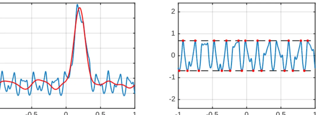
3. High-level software framework of numerical computing with functions. Whereas existing algorithms for best approximation produce parameters that describe an approximating function, our algorithm produces the function itself — a representation of it in Chebfun that can then be used for further computa-tion. Thus we can calculate a best approximation in a single line of Chebfun, and further operations like evaluation, differentiation, maximization, or other transformations are available with equally simple commands. For example, our algorithm makes it possible to compute and plot the degree 10 minimax approximation of the function f(x) = 1/(2 + sin 22πx) + (1/2) cos 13πx+ 5e−80(x−0.2)2
with these commands:
-1 -0.5 0 0.5 1 -1 0 1 2 3 4 5 6 -1 -0.5 0 0.5 1 -2 -1 0 1 2
Fig. 1.The functionf(x) = 1/(2 + sin 22πx) + (1/2) cos 13πx+ 5e−80(x−0.2)2
and its degree10 best trigonometric approximation (left). The error curve equioscillates between22extrema, marked by red dots (right).
>> x = chebfun('x');
>> f = 1./(2+sin(22*pi*x))+cos(13*pi*x)/2+5*exp(-80*(x-.2).^2); >> tic, t = trigremez(f, 10); toc
Elapsed time is 1.968467 seconds. >> norm(f-t, inf)
ans = 6.868203985976071e-01 >> plot(f-t)
The plot of the functionf, its best approximationt10 and the resulting error curve are shown in Figure 1.
The outline of the paper is as follows. In Section 2, we define the problem and the associated vector space of trigonometric polynomials and present classical results guaranteeing the existence and uniqueness of the best approximation. In Section 3, we present the theoretical background of the Remez algorithm for the trigonometric case. In Section 4 we present our algorithm and its implementation details. Section 5 consists of numerical examples. In Section 6 we conclude the paper while indicating future directions.
2. Trigonometric polynomials and best approximation. Before defining trigonometric polynomials, we define the domain on which these functions live, the quotient space
T=R/2πZ,
which is topologically equivalent to a circle. Loosely speaking, a functionf defined onTis a 2π-periodic function onR. To be precise, we shall think of the function as defined on the interval [0,2π). A subset of [0,2π) will be considered open or closed if the corresponding set inTis open or closed. Throughout this paper, we speak casually of the interval [0,2π) with the understanding that we are actually consideringT.
By a trigonometric polynomial of degreen, we mean a functiont: [0,2π)→Rof the form∗: (2.1) t(θ) =a0+ n X k=1 (akcoskθ+bksinkθ), where{ak}and{bk}are real numbers.
We shall denote the 2n+ 1 dimensional vector space of all trigonometric polyno-mials of degreenor less byTn. We note that the set{1,cosθ,sinθ, . . . ,cosnθ,sinnθ} is a basis forTn.
We are interested in finding the best approximation in the∞-norm,
(2.2) ktk∞:= sup
θ∈[0,2π) |t(θ)|.
The problem: Given a real-valued continuous function f : T→R and a non-negative integern, find the function t∗∈ Tn such that
(2.3) kf−t∗k
∞≤ kf−tk∞, ∀t∈ Tn.
∗Trigonometric polynomials are in general complex-valued, but we shall only consider the real-valued case. The theory of minimax approximation of complex-real-valued functions is considerably different.
A best approximation exists, as can be proven easily; see for instance [13]. It is also unique. The proof of uniqueness relies on a property of the spaceTn which we now define.
2.1. The Haar condition. The Haar condition is a certain property of a finite dimensional vector space of functions. LetC(Ω) be the space of real-valued continuous functions on a compact set Ω and let V be a finite dimensional subspace of C(Ω). If V satisfies the Haar condition, then the uniqueness of the best approximation to a given f ∈ C(Ω) from V is guaranteed. The existence of a best approximation is provable under less restrictive conditions [13]. However, for the uniqueness of the best approximation, the Haar condition becomes important.
There are various ways of characterizing the Haar condition; see [9] and [13].
Definition 1. Let V be an n dimensional vector subspace of C(Ω). Then V
satisfies the Haar condition if for every nonzerot∈V, the number of roots of tin Ω is strictly less than n.
This is equivalent to the following [9]:
Definition 2. Let V be an n dimensional vector subspace of C(Ω) and let
{θk}nk=1 be any set of ndistinct points in[a, b]. Then V satisfies the Haar condition if there is a unique function t in V which interpolates arbitrary data {fi}n
i=1, i.e.
t(θi) =fi, i= 1,2, . . . , n.
Equivalently, V satisfies the Haar condition if for any basis {ti : i= 1,2, . . . , n} of V and any distinct set of n points in Ω, the associated Vandermonde matrix is nonsingular.
Theorem 3. The space Tn satisfies the Haar condition.
Proof. We can prove this theorem by showing that any nonzero trigonometric polynomial t∈ Tn has at most 2n roots inT, i.e. in the interval [0,2π)[17, Chapter X]. We writet as (2.4) t(θ) =a0+ n X k=1 (akcoskθ+bksinkθ) = n X k=−n ckeikθ.
Leteiθ=zand consider the function
(2.5) p(z) =einθt(θ),
an algebraic polynomial of degree 2n in the variablez. The result now follows from the fundamental theorem of algebra.
It is interesting to note that the very similar vector spaces generated by the linear combinations of vectors inTn and just one of the functions cos(n+ 1)θ or sin(n+ 1)θ
do not satisfy the Haar condition. For a simple example, consider the vector space generated by linear combinations of vectors inT0and say, cosθ, i.e. the vector space
span{1,cosθ}.
We now try to interpolate data{1,1}at two points, where the first pointθ1is arbitrary in (0, π) and the second pointθ2is defined byθ2= 2π−θ1. We now easily see that the constant function 1 and the function cosθ/cosθ1 both interpolate the data. These are distinct interpolants and hence the Haar condition is not satisfied.
Another way of proving that the Haar condition is not satisfied by this vector space is by noting that the function cosθ, which lies in this space, has two roots in [0,2π), while the dimension of the vector space itself is also 2.
3. The Remez algorithm for periodic approximations: Theoretical back-ground. The Remez algorithm, also called the exchange algorithm, is a nonlinear iterative procedure which, in its usual setting, calculates the best approximation of a given function f ∈ C([a, b]) from the vector space Pn of algebraic polynomials of degreenor less. For a givenf, starting from an arbitrary initial condition, the algo-rithm converges to the best approximation off inPn, and a proof of its convergence can be found in [13]. In the following sections we will see how the same algorithm, with certain modifications, can be used to find best approximations of continuous periodic functions inTn.
Let us now look at the details of the algorithm. We shall closely follow [13], adapting its discussion of algebraic polynomials to our problem of trigonometric poly-nomials.
Lett∗be the best approximation of a continuous periodic functionf ∈C([0,2π))
from the spaceTn. Lettk be thekthtrial approximation in the iterative sequence and define the corresponding error at thekthiteration as
(3.1) ek(θ) =f(θ)−tk(θ), 0≤θ <2π.
Since we are approximating in the ∞-norm, the set of points at whichek takes its extreme values is of interest. Let us denote this set byEk,
(3.2) Ek={θ:θ∈[0,2π), |ek(θ)|=kek(θ)k∞}.
3.1. A sufficient condition for optimality. We suppose that at thekthstep,
tk is not the best approximation. We can then write the best approximationt∗ as (3.3) t∗(θ) =tk(θ) +αt(θ),
for some trigonometric polynomialt ∈ Tn, such thatktk∞ = 1 and, without loss of
generality, some realα >0. With this notation we have (3.4) e∗=f −t∗=f−t
k−αt=ek−αt.
By definition of the best approximation, forθ∈Ek,e∗ is strictly less than e
k in absolute value:
(3.5) |e∗(θ)|=|e
k(θ)−αt(θ)|<|ek(θ)|, θ∈Ek.
Sinceα >0, this implies that for every θ∈Ek,t(θ) has the same sign asek(θ). Thus, if tk is not the best approximation, there is a function t ∈ Tn which has the same sign asek at the points inEk, i.e.
(3.6) [f(θ)−tk(θ)]t(θ)>0, θ∈Ek.
3.2. A necessary condition for optimality. We now prove the converse of the above statement: if there exists a trigonometric polynomialt∈ Tn for which the condition (3.6) holds, thentkis not the best approximation, i.e. there exists a positive value ofαsuch that
(3.7) kf−(tk+αt)k∞<kf−tkk∞.
We again closely follow [13]. LetE denote a closed subset of the interval [0,2π), which as always means more precisely a closed subset of T. Also, let α > 0 and without loss of generality, assume thatt∈ Tn satisfies the bound
(3.8) |t(θ)| ≤1, 0≤θ <2π.
We defineEo ⊂E as the set of points in E for which ek(θ) and t(θ) have opposite signs:
(3.9) Eo={θ∈E:t(θ)ek(θ)≤0}.
Since Eo is closed, any continuous function attains its bounds on Eo, and we can therefore define the numberdas
(3.10) d:= max
θ∈Eo
|ek(θ)|.
In caseEo is empty, we defined= 0. SinceEo∩Ek is empty, we have
(3.11) d <max
θ∈E|ek(θ)|. We now prove that the inequality
(3.12) max θ∈E|f(θ)−tk(θ)−αt(θ)|<maxθ∈E|f(θ)−tk(θ)| holds for (3.13) α=1 2 max θ∈E|ek(θ)| −d .
SinceE is closed, we may letγ be an element ofE such that (3.14) |f(γ)−tk(γ))−αt(γ)|= max
θ∈E|f(θ)−tk(θ)−αt(θ)|. Ifγ∈Eo, we have
max
θ∈E|f(θ)−tk(θ)−αt(θ)|=|f(γ)−tk(γ)|+|αt(γ)| ≤d+α <maxθ∈E|ek(θ)|, where the last bound follows by inserting the value ofd+αfrom (3.13).
On the other hand if γ /∈Eo then the signs ofek(γ) and t(γ) are the same, and we get the strict inequalities
(3.15) max
θ∈E|f(θ)−tk(θ)−αt(θ)|<max{|ek(γ)|,|αt(γ)|}<maxθ∈E|ek(θ)|, where in the last inequality, we have again used the definition ofα from (3.13) and the fact thattis bounded by 1. Therefore, we have shown that (3.12) holds.
We summarize the last two conditions as the following theorem.
Theorem 4. Let E be a closed subset of[0,2π), i.e. closed inT. Let tk be any element of Tn and let Ek be the subset of E where the error ek(θ) = f(θ)−tk(θ) takes its maximum absolute value. Then tk is the function in Tn that minimizes the expression
(3.16) max
θ∈E|f(θ)−t(θ)|, t∈ Tn, if and only if there is no functiont∈ Tn such that
(3.17) [f(θ)−tk(θ)]t(θ)>0, θ∈Ek. Proof. In the discussion above.
3.3. Characterization of the best approximation. Theorem 4 tells us that in order to find out if a trial approximationtk is the best approximation or not, one only needs to consider the extreme values of the error functionek(θ) =f(θ)−tk(θ). Specifically, one should ask if the condition (3.6) holds for some function t ∈ Tn. This allows us to characterize the best approximation by the sign changes of the error function. Since we are working in the space of trigonometric polynomials, condition (3.6) is rather easy to test. We make use of the fact that any function in Tn has at most 2n sign changes† in T. Therefore, if the error function changes sign more
than 2n times as θ ranges in Ek, then tk is the best approximation. Conversely, if the number of sign changes does not exceed 2n, then we can choose the zeros of a trigonometric polynomial to construct t in Tn so that the condition (3.6) is satisfied. This result is usually called the minimax characterization theorem [13] or the equioscillation theorem, which we state below.
Theorem 5. (Equioscillation) Letf be a continuous periodic function on[0,2π). Thent∗ is the best approximation off fromTn if and only if there exist2n+ 2points
{θi, i= 1,2, . . . ,2n+ 2} such that the following conditions hold: (3.18) 0≤θ1< θ2<· · ·< θ2n+2<2π,
(3.19) |f(θi)−t∗(θi)|=kf−t∗k
∞, i= 1,2, . . . ,2n+ 2,
and
(3.20) f(θi+1)−t∗(θi+1) =−[f(θi)−t∗(θi)], i= 1,2, . . . ,2n+ 1.
Proof. See [4] or [13].
A discrete version of the above theorem also holds, which we state below as a separate theorem. As we will see, this is one of the key results used by the Remez algorithm.
Theorem 6. Let f be a continuous periodic function on[0,2π)and let 0≤θ1<
θ2 < · · · < θ2n+2 < 2π be 2n+ 2 points in [0,2π). Then t∗ ∈ Tn minimizes the expression
(3.21) max
i |f(θi)−t(θi)|, t∈ Tn,
†For example the function sin(θ) has exactly 2 sign changes inT, one atθ= 0 and another at
if and only if
(3.22) f(θi+1)−t∗(θi+1) =−[f(θi)−t∗(θi)], i= 1,2, . . . ,2n+ 1.
Proof. See [13].
Theorem 7. Let the conditions of Theorem 5 hold and let t∗ be any element of
Tn such that the conditions
(3.23) sign[f(θi+1)−t∗(θi+1)] =−sign[f(θi)−t∗(θi)], i= 1,2, . . . ,2n+ 1,
are satisfied. Then the inequalities min i |f(θi)−t ∗(θi)| ≤min t∈Tn max i |f(θi)−t(θi)| ≤mint∈Tn kf−tk∞≤ kf −t∗k∞ (3.24)
hold. Also, the first inequality is strict unless all the numbers {|f(θi)−t∗(θi)|, i =
1,2, . . . ,2n+ 2} are equal. Proof. See [13].
The next theorem is contained in Theorem 7. However, to clearly establish a link between the sign alternation of the error function ek on a discrete set and the error in the best approximatione∗, we state it separately.
Theorem 8. (de la Vall´ee Poussin) Lettk ∈ Tnand0≤θ1< θ2<· · ·< θ2n+2< 2π be2n+ 2 points in[0,2π)such that the sign of the errorf(θi)−tk(θi)alternates asi varies from1to2n+ 2. Then, for everyt∈ Tn,
(3.25) min
i |f(θi)−tk(θi)| ≤maxi |f(θi)−t(θi)|
Also, the inequality is strict unless all the numbers{|f(θi)−tk(θi)|, i= 1,2, . . . ,2n+2} are equal.
The above theorem tells us that if we construct tk ∈ Tn such that the error ek alternates its sign as above, then a lower bound for e∗ can be easily obtained: let t=t∗ in the theorem above and we get
(3.26) min
i |f(θi)−tk(θi)| ≤maxi |f(θi)−t
∗(θi)| ≤ kf−t∗k
∞≤ kf−tkk∞.
This also gives us a way of boundingkf−tkk∞bykf−t∗k∞. For it follows from the
inequalities above that
1≤ kf −t
∗k ∞
mini|f(θi)−tk(θi)|
,
and now multiplying both sides of the inequality above by kf −tkk∞, we get the
bound (3.27) kf−tkk∞≤ kf −tkk ∞ mini|f(θi)−tk(θi)| kf −t∗k ∞.
4. The Remez (exchange) algorithm for periodic functions: Imple-mentation details. The Remez algorithm, at each iteration, finds a set of points
Rk ={θi, i= 1,2, . . . ,2n+ 2}and a trigonometric polynomial tk ∈ Tn such that the conditions of Theorem 6 are satisfied. We will call the setRk thekth reference.
To start the algorithm, an initial referenceR1 is chosen. This can be any set of points that satisfies:
(4.1) 0≤θ1< θ2<· · ·< θ2n+2<2π.
The exchange algorithm is guaranteed to converge from any starting reference [13]. However, the number of iterations taken to achieve a certain accuracy is greatly affected by the choice of the initial reference. For the present case of trigonometric polynomials, we start by choosing 2n+ 2 equally spaced points in [0,2π).
4.1. Computation of the trial polynomial using trigonometric interpo-lation. At the start of each iteration, a new reference is available which is different from the references of all the previous iterations. Given a reference Rk, first the trigonometric polynomialtk is constructed that minimizes the expression
(4.2) max
i=1,2,...,2n+2|f(θi)−tk(θi)|, tk∈ Tn. Theorem 6 shows that this can be done by solving the linear system (4.3) f(θi)−tk(θi) = (−1)i−1h
k, i= 1,2, . . . ,2n+ 2, which also defines the unknownlevelled reference error hk.
However, instead of solving the linear system, we convert this problem to an interpolation problem. First, note that there are 2n+ 2 unknown parameters: the unknownhk and the 2n+ 1 unknown coefficients of the trigonometric polynomial tk. It turns out the levelled reference error hk can be found explicitly without solving the linear system (see Appendix). Once this is done, we can re-write (4.3) as an interpolation problem:
(4.4) tk(θi) =f(θi) + (−1)i−1hk, i= 1,2, . . . ,2n+ 2,
At a first look, it seems that this problem is overdetermined: it has 2n+ 2 data points to interpolate and only 2n+ 1 degrees of freedom in the coefficients of tk. However, sincehk has been found as a part of the original problem, we can discard any oneθifrom (4.4) and find the unique interpolant to the remaining data. The result is an interpolant that automatically interpolates the data at the discarded node.
This interpolation problem is solved using the trigonometric barycentric formula of the second kind [2], [3]:
(4.5) tk(θ) = P2n+1 i=1 wicsc12(θ−θi)tk(θi) P2n+1 i=1 wicsc12(θ−θi) , where (4.6) w−i 1= 2n+1 Y j=1,j6=i sin1 2(θi−θj).
The formula (4.5) is implemented in Chebfun [16] and thus we can compute the interpolanttk very easily. In fact, the complete code for constructingtk is as follows:
dom = [0, 2*pi];
sigma = ones(2*n+2, 1); sigma(2:2:end) = -1;
hk = (w'*fk) / (w'*sigma); % Levelled reference error
uk = (fk - hk*sigma); % Values to be interpolated
tk = chebfun(@(t) trigBary(t, uk, xk, dom), dom, 2*n+1, 'trig');
4.2. Finding the new reference. The next step of the algorithm is to find a new referenceRk+1. From Theorem 7, we see that the following bound holds: (4.7) |hk| ≤ kf−t∗k∞≤ kf−tkk∞.
By increasing|hk|, we get closer and closer to the best approximation. The exchange algorithm tries to choose the new reference so as to maximize the magnitude of the levelled reference error hk at each iteration. One might think then that a classical optimization algorithm should be used to solve this problem. However, according to [13], the structure ofhk is such that the standard algorithms of optimization are not efficient.
We now look at ways of increasing the levelled reference error so that|hk+1|>|hk|. Let the new reference be Rk+1 = {ζi, i = 1,2, . . . ,2n+ 2}, and let the new trial approximation be tk+1. To ensure |hk+1| > |hk|, Theorem 7 tells us that the new reference must be chosen such that the old trial polynomial tk oscillates on it (not necessarily equally) with a magnitude greater than or equal to|hk|:
(4.8) sign[f(ζi+1)−tk(ζi+1)] =−sign[f(ζi)−tk(ζi)], i= 1,2, . . . ,2n+ 1,
and
(4.9) |hk| ≤ |f(ζi)−tk(ζi)|, i= 1,2, . . . ,2n+ 2,
where at least one of the inequalities is strict. If the above conditions are satisfied, then it follows from Theorem 8 that
(4.10) |hk| ≤min
i |f(ζi)−tk(ζi)|<maxi |f(ζi)−tk+1(ζi)|=|hk+1|.
This gives us a number of possibilities for choosing the new referenceRk+1. In the so called one-point exchange algorithm, it is obtained by exchanging a single point ofRk with the global maximum of the error functionek in such a way that the oscillation of the error (4.8) is maintained. The other extreme is to define all points of the new reference as local extrema of the error ek in such a way that conditions (4.8) and (4.9) are satisfied. Methods that can change every reference point at every iteration are usually more efficient than the one-point exchange algorithm in the sense that fewer iterations are required for convergence. In this paper, we will not discuss the convergence properties of exchange algorithms; see [13].
Regardless of what exchange strategy is chosen, one needs to compute local or global extrema of the error functionek=f−tk. This is where our algorithm, following [10], uses Chefun’s root finder. This algorithm has three steps.
1. Differentiate the error function. Since the functions f and tk are periodic, the error function ek is also periodic. We can therefore compute e
′
k in a numerically stable way by using the Fourier expansion coefficients ofek. This is automated in Chebfun via the overloadeddiffcommand.
ekp = diff(f-tk);
2. Expansion in Chebyshev basis. To find the roots of a periodic chebfun, one can solve a companion matrix eigenvalue problem. However, the straight-forward implementation of this process will lead to anO(n3) algorithm [16]. To use Chebfun’s O(n2) recursive interval subdivision strategy root finding algorithm, the function is first converted to a nonperiodic chebfun. This can be done by issuing the command:
g = chebfun(ekp);
To be precise, the above line of code computes a Chebyshev interpolant of the function ekp, which is as good as a Chebyshev series expansion up to machine precision [15].
3. Find the roots. Finally, we use the Chebyshev coefficients obtained in step 2 to compute the roots:
r = roots(g);
The above line computes roots as eigenvalues of a colleague matrix [1], [15]. The above three steps were spelled out to give algorithmic details. However, in Chebfun, they are all combined in a single line of code:
r = minandmax(f-tk, 'local');
Once the roots are computed, we can find the new reference Rk+1 using either the one-point exchange or the multiple point exchange strategy.
Our algorithm uses the multiple point exchange strategy. Let Wk be the set of local extrema ofek. We form the setSk={ζ:ζ∈Wk∪Rk,|ek(ζ)| ≥ |hk|}. We then order the points in Sk, and for each subset of consecutive points with the same sign, we keep only one for which|ek|is maximum. From this collection of points,Rk+1 is formed by selecting 2n+ 2 consecutive points that include the global maximum ofek. This completes one iteration of the exchange algorithm. The algorithm terminates whenkek+1k∞ is within a prescribed tolerance of|hk|.
5. Numerical examples. Let us now look at some examples. The Chebfun commandtrigremez(f, n)finds the degreenbest approximation of a periodic con-tinuous chebfunfon its underlying domain[a, b]:
t = trigremez(f, n);
Here is a basic example for a function on the default interval [−1,1]:
f = chebfun(@(x) exp(sin(8*pi*x)) + 5*exp(-40*x.^2), 'trig' ) t = trigremez(f, 4);
−1 −0.5 0 0.5 1 0 2 4 6 8 −1 −0.5 0 0.5 1 −4 −2 0 2 4
Fig. 2. The functionf(x) =esin 8πx
+ 5e−40x2
, its degree4best approximation (left) and the equioscillating error curve (right).
An interesting feature oftrigremezis that we can use it with nonperiodic as well as periodic chebuns. As long as a function is continuous in the periodic sense, i.e. the function values are same at the endpoints, the theorems stated in the previous sections hold and it does not matter how whether we represent it as a Chebyshev (aperiodic) or a Fourier (periodic) expansion.
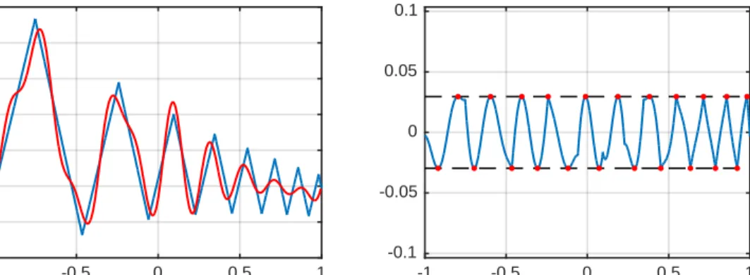
Here is a modified version of an example of a zig-zag function taken from [15]. To make the function continuous across the periodic boundary, we have subtracted off an appropriate linear term:
-1 -0.5 0 0.5 1 -0.05 0 0.05 0.1 0.15 0.2 0.25 0.3 -1 -0.5 0 0.5 1 -0.1 -0.05 0 0.05 0.1
x = chebfun('x');
g = cumsum(sign(sin(20*exp(x)))); m = (g(1)-g(-1))/2;
f = g - m*x;
t = trigremez(f, 10);
We can see the approximation and the error curve in Figure 3.
-1 -0.5 0 0.5 1 -0.05 0 0.05 0.1 0.15 0.2 0.25 0.3 -1 -0.5 0 0.5 1 -0.02 -0.01 0 0.01 0.02
Fig. 4. Degree20approximation of the same function.
Figure 4 is for the same problem but with a higher degree of approximation.
-1 -0.5 0 0.5 1 0 0.2 0.4 0.6 0.8 1 -1 -0.5 0 0.5 1 -0.01 -0.005 0 0.005 0.01
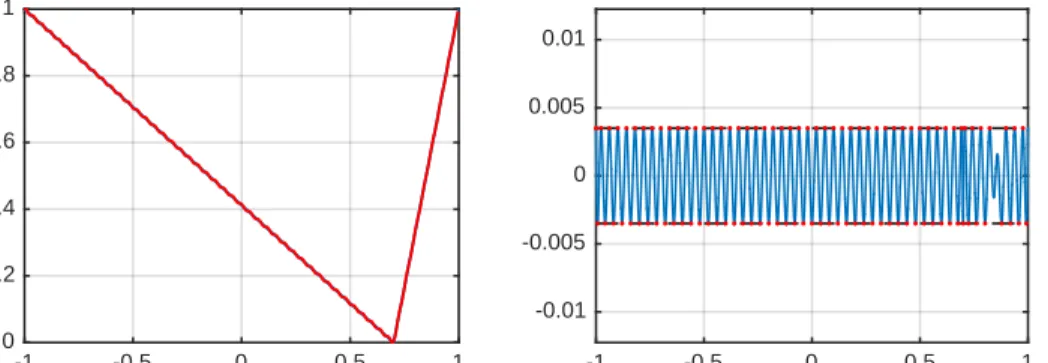
Fig. 5. The shifted absolute value function and its degree 50best approximation. The corre-sponding error curve is also shown.
Here is another example featuring the absolute value function, shifted to break the symmetry:
x = chebfun('x');
f = (-x+0.7)/(1+0.7).*(x<0.7) + (x-0.7)/(1-0.7).*(x>=0.7); t = trigremez(f, 50);
The plots can be seen in Figure 5.
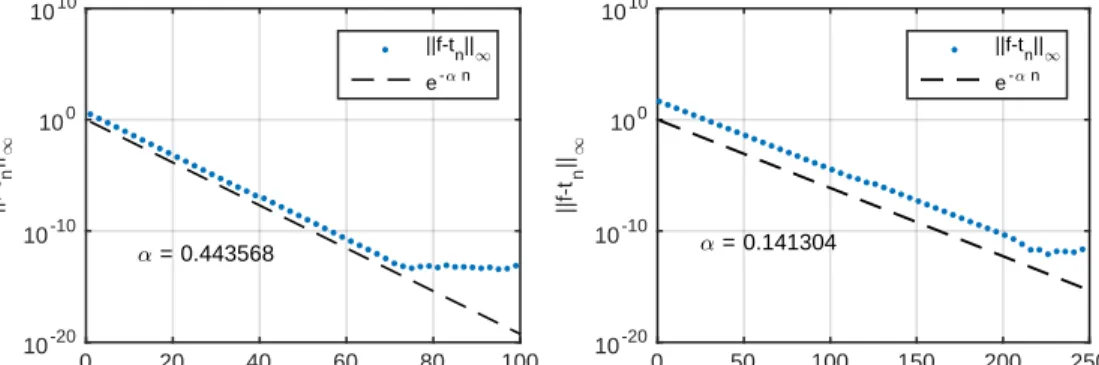
It is well known that for functions analytic on [0,2π], the best approximation error decreases exponentially at the rate of O(e−αn), where n is the degree of the best approximation andαis the distance of the real line from the nearest singularity of the function [16]. (More precisely we get O(e−αn) if f is bounded in the strip of analyticity defined by the nearest singularity. If not, we still have O(e−(α−ǫ)n) for any ǫ > 0, and there is no need for the ǫ if the closest singularities are just simple poles.) As an example, we consider the functionf(θ) = (b+ cosθ)−1which has poles in the complexθ-plane along the line θ= 1. For b = 1.1 the half-width of the strip of analyticity isα≃0.443568, while forb= 1.01, α≃0.141304. In Figure 6, we see that the numerical decay of the error matches the predicted decay beautifully.
degree of the polynomial
0 20 40 60 80 100 ||f-t n || 1 10-20 10-10 100 1010 , = 0.443568 ||f-tn|| 1 e-, n
degree of the polynomial
0 50 100 150 200 250 ||f-t n || 1 10-20 10-10 100 1010 , = 0.141304 ||f-tn|| 1 e-, n
Fig. 6. Error in the best approximation off(θ) = (b+ cosθ)−1 as a function of the degree of the approximating polynomial. b= 1.1for the plot on the left,b= 1.01for the plot on the right.
-3 -2 -1 0 1 2 3 -0.6 -0.4 -0.2 0 0.2 0.4 0.6
Fig. 7.Almost sinusoidal error curve produced while approximatingf(θ) = (1.01−cosθ)−1by a degree40trigonometric polynomial.
Best approximations in spaces of algebraic polynomials yield error curves that look approximately like Chebyshev polynomials, and indeed, there are theorems to the effect that for functions satisfying appropriate smoothness conditions, the error curves approach multiples of Chebyshev polynomials as the degree approaches infinity. In trigonometric rather than algebraic best approximation, however, the error curves tend to look like sine waves, not Chebyshev polynomials. To the experienced eye,
this can be quite a surprise. The following example illustrates this, and the almost sinusoidal error curve can be seen in Figure 7.
f = chebfun('1./(1.01-cos(x))',[-pi,pi],'trig'); plot(f-trigremez(f,40)), ylim([-1 1])
6. Conclusion and future work. In this paper, we have presented a Remez algorithm for finding the minimax approximation of a periodic function in a space of trigonometric polynomials. Two key steps are trigonometric interpolation and deter-mining the extrema of the error function. We use the second kind barycentric formula for the former and Chebfun’s root finding algorithm for the later. The algorithm is already a part of Chebfun‡ and perhaps more than applications, its greatest use is for
fundamental studies in approximation theory.
Our algorithm can easily be modified to design digital filters with real but asym-metric frequency responses, see [8]. Specifically, this can be achieved by making sure that during the iterations of the algorithm, no point of the reference set lies in the don’t-care regions specified. This results in best approximation on a compact subset of [0,2π). Details will be reported elsewhere.
The computation of best approximations via the Remez algorithm and its variants is a nonlinear process. An alternative is the Carath´eodory-Fej´er (CF) method [15], based on singular values of a Hankel matrix of Chebyshev coefficients, which has been used to compute near-best approximations of algebraic polynomials [6]. We are working on a CF algorithm for periodic functions based on the singular values of a matrix of Fourier coefficients.
Appendix. Formula for the levelled reference error hk. Let us again consider the linear system (4.3):
(A.1) f(θj)−tk(θj) = (−1)j−1hk, j= 1,2, . . . ,2n+ 2,
where the points θj ∈[0,2π) are distinct. The polynomial tk is of degree n, which implies that there are 2n+ 1 unknown parameters needed to completely determine
tk. However, the linear system consists of 2n+ 2 equations with 2n+ 1 unknowns corresponding to tk and the unknown levelled error hk. We will now show how the unknownhk can be determined without solving the linear system.
We begin by expressing the degree n trigonometric polynomial tk in a trigono-metric Lagrangian basis. Since there is one extra collocation point, say θj, we may define thejthset of basis functions β
j as (A.2) βj= n lij∈ Tn, i= 1,2, . . . , j−1, j+ 1, . . . ,2n+ 2. o , where (A.3) lji(θ) := 2n+2 Y ν=1,ν6=i,j sin12(θ−θν) sin12(θi−θν) .
Note that the function lji(θ) is a degree n trigonometric polynomial that takes the value 1 atθ=θi and 0 at all other nodes except θ=θj, where it takes an unknown
value. Therefore for a givenj∈ {1,2, . . . ,2n+ 2}, the polynomialtk can be expressed as (A.4) tk(θ) = 2n+2 X i=1,i6=j tk(θi)lij(θ)
Using the above expression to evaluatetkatθj, we can write the original linear system (A.1) as: (A.5) f(θj)− 2n+2 X i=1,i6=j tk(θi)lij(θj) = (−1) j−1h k, j= 1,2, . . . ,2n+ 2.
We can simplify the numberlij(θ) by writing
lji(θj) = 2n+2 Y ν=1,ν6=i,j sin1 2(θj−θν) sin1 2(θi−θν) (A.6) = Q2n+2 ν=1,ν6=jsin 1 2(θj−θν) Q2n+2 ν=1,ν6=isin 1 2(θi−θν) ×sin 1 2(θi−θj) sin1 2(θj−θi) =−wi wj , (A.7) where (A.8) w−j1= 2n+2 Y ν=1,ν6=j sin1 2(θj−θν). This allows us to write (A.5) as
(A.9) f(θj)wj− 2n+2
X
i=1,i6=j
tk(θi)wi= (−1)j−1wjhk, j= 1,2, . . . ,2n+ 2. Now summing overj we get
(A.10) 2n+2 X j=1 f(θj)wj− 2n+2 X j=1 2n+2 X i=1,i6=j tk(θi)wi= 2n+2 X j=1 (−1)j−1w jhk.
The double sum above collapses to zero when we use the fact that (A.11)
2n+2
X
i=1
tk(θi)wi= 0. We can therefore rearrange (A.10) to writehk as
(A.12) hk = P2n+2 j=1 wjf(θj) P2n+2 j=1 (−1)j−1wj .
which is the required closed form expression.
[1] Z. Battles and L. N. Trefethen,An extension of MATLAB to continuous functions and operators, SIAM Journal on Scientific Computing, 25 (2004), pp. 1743–1770.
[2] J.-P. Berrut,Baryzentrische Formeln zur trigonometrischen Interpolation (i), Zeitschrift f¨ur angewandte Mathematik und Physik, 35 (1984), pp. 91–105.
[3] J.-P. Berrut and L. N. Trefethen,Barycentric Lagrange interpolation, SIAM Review, 46 (2004), pp. 501–517.
[4] E. W. Cheney,Introduction to Approximation Theory, AMS Chelsea Publishing, Providence, Rhode Island, 1998.
[5] T. A. Driscoll, N. Hale, and L. N. Trefethen, Chebfun Guide, Pafnuty Publications, Oxford, 2014.
[6] M. H. Gutknecht and L. N. Trefethen,Real polynomial Chebyshev approximation by the Carath´eodory-Fej´er method, SIAM Journal on Numerical Analysis, 19 (1982), pp. 358–371. [7] L. J. Karam and J. H. McClellan,Complex Chebyshev approximation for FIR filter design, IEEE Transactions on Circuits and Systems II: Analog and Digital Signal Processing, 42 (1995), pp. 207–216.
[8] M. McCallig, Design of digital FIR filters with complex conjugate pulse responses, IEEE Transactions on Circuits and Systems, 25 (1978), pp. 1103–1105.
[9] G. Meinardus,Approximation of Functions: Theory and Numerical Methods, Springer, 1967. [10] R. Pach´on and L. N. Trefethen,Barycentric-Remez algorithms for best polynomial
approx-imation in the chebfun system, BIT Numerical Mathematics, 49 (2009), pp. 721–741. [11] T. Parks and J. McClellan,Chebyshev approximation for nonrecursive digital filters with
linear phase, IEEE Transactions on Circuit Theory, 19 (1972), pp. 189–194.
[12] S.-C. Pei and J.-J. Shyu,Design of complex FIR filters with arbitrary complex frequency re-sponses by two real Chebyshev approximations, IEEE Transactions on Circuits and Systems I: Fundamental Theory and Applications, 44 (1997), pp. 170–174.
[13] M. J. D. Powell,Approximation Theory and Methods, Cambridge University Press, 1981. [14] L. Rabiner, J. H. McClellan, and T. W. Parks,FIR digital filter design techniques using
weighted Chebyshev approximation, Proceedings of the IEEE, 63 (1975), pp. 595–610. [15] L. N. Trefethen,Approximation Theory and Approximation Practice, SIAM, 2013. [16] G. B. Wright, M. Javed, H. Montanelli, and L. N. Trefethen,Extension of Chebfun to
periodic functions, SIAM J. Sci. Comp., (submitted).
[17] A. Zygmund,Trigonometric Series, vol. I & II combined, Cambridge University Press, sec-ond ed., 1988.