広島大学学術情報リポジトリ
Hiroshima University Institutional Repository
Title
Image representation for generic object recognition usinghigher-order local autocorrelation features on posterior probability imagesAuther(s)
Matsukawa, Tetsu; Kurita, TakioCitation
Pattern Recognition , 45 (2) : 707 - 719Issue Date
2012DOI
10.1016/j.patcog.2011.07.018Self DOI
URL
http://ir.lib.hiroshima-u.ac.jp/00034797Right
This is a preprint of an article submitted forconsideration in Pattern Recognition (c) 2012 Elsevier B.V. ; Pattern Recognition is available online at ScienceDirect with the open URL of your article;Relation
Image representation for generic object recognition
using higher-order local autocorrelation features on
posterior probability images
Tetsu Matsukawa∗,a, Takio Kuritab
aGraduate School of Systems and Information Engineering, University of Tsukuba, 1-1-1
Tennodai, Tsukuba, Ibaraki 305-8573, Japan
bNeuroscience Research Institute, National Institute of Advanced Industrial Science and
Technology, 1-1-1 Umezono, Tsukuba, Ibaraki 305-8568, Japan
Abstract
This paper presents a novel image representation method for generic object recognition by using higher-order local autocorrelations on posterior proba-bility images. The proposed method is an extension of the bag-of-features approach to posterior probability images. The standard bag-of-features ap-proach is approximately thought of as a method that classifies an image to a category whose sum of posterior probabilities on a posterior probability image is maximum. However, by using local autocorrelations of posterior probability images, the proposed method extracts richer information than the standard bag-of-features. Experimental results reveal that the proposed method exhibits higher classification performances than the standard bag-of-features method.
Key words: Image recognition, Higher-order local autocorrelation feature, Bag-of-features, Posterior probability image
∗Corresponding author. Tel.: +81 029 861 5080; fax: +81 029 861 5842
1. Introduction
Generic object recognition technologies have many possible applications such as automatic image search. However, generic object recognition in-volves some very difficult problems, because one has to deal with inherent object/scene variations as well as difficulties in viewpoint, lighting, and oc-clusion. Thus, although many methods of generic object recognition have been developed so far, the classification performance of these conventional methods are still insufficient, and a method that can achieve high classifica-tion accuracy is strongly desired.
The bag-of-features approach is the most popular approach for generic ob-ject recognition [1] because of its simplicity and effectiveness. This approach is originally inspired from the text recognition method called “bag-of-words,” and this method treats an image as an orderless collection of quantized ap-pearance descriptors extracted from local patches. The main steps of the bag-of-features are (1) detection and description of image patches. (2) as-signing patch descriptors to a set of predetermined codebooks with a vector quantization algorithm, (3) constructing a bag of features, which counts the number of patches assigned to each codebook, and (4) applying a classifier by treating the bag of features as the features vector and thus determining the category which an image can be assigned.
It is known that the bag-of-features method is robust with regard to background clutter, pose changes, and intraclass variations and offers good classification accuracy. However, several problems exist with regard to its application to image representation. To solve these problems, many methods
have been proposed. These methods include spatial pyramid binning that utilizes location information [2], higher level codebook creation based on local co-occurrence of codebooks [3, 4, 5], improvement of codebook creation[6, 7, 8, 9], and image matching based on the region of interest [10]. All these methods are based on the histogram of local appearance, and information pertaining to semantic class labels is not used for feature representation.
In this paper, we present a novel method that improves upon the bag-of-features method. The main feature of the proposed method is that it utilizes posterior probability images for semantic feature extraction. The standard bag-of-features method is approximately thought of as a method that classifies an image to a category whose sum of posterior probabilities on a posterior probability image is maximum. This method does not utilize local co-occurrence of posterior probability images. We applied higher-order local autocorrelations [11] on posterior probability images, so as to extract richer information regarding these images. We call this image representa-tion method as “probability higher-order local autocorrelarepresenta-tions (PHLAC).” PHLAC has certain desirable properties for image recognition, namely, shift invariance, additivity, and synonymy [12] invariance. Furthermore, the fea-ture dimension of PHLAC is independent of the codebook size, and it depends on the class number, which is usually much smaller than the codebook size. We confirm that the classification performance of this image representation method (PHLAC) is considerably better than that of the standard bag-of-features method and offers competitive performance to the bag-of-bag-of-features using spatial information.
cal-culated from multiple image features. We call this image representation method as “multiple features probability higher-order local autocorrelations (MFPHLAC).” It is confirmed that MFPHLAC can achieve a slightly better performance than PHLAC.
This paper is an extended version of the paper cited in [13]. The exten-sions include an algorithm of MFPHLAC, experimental results of multiple spatial intervals, and discussions on feature dimension.
2. Related Studies
We intend to improve the classification accuracy of the bag-of-features method by introducing local co-occurrence and information pertaining to semantic class labels. From these points of view, the following related studies have been reported.
Image feature extraction using local co-occurrence is recognized as an im-portant concept [11] for image recognition. Recently, several methods have been proposed using local co-occurrence. These methods are categorized as the methods that use feature level co-occurrence and those that use code-book level co-occurrence. The examples of the methods that use feature level co-occurrence are the local self similarity method [14], gradient local auto-correlations (GLAC) [15], and color index local autocorrelation (CILAC) [16]. Low-level co-occurrence of image properties such as edge direction and color can be represented by these features, whereas the codebook level co-occurrence can capture the co-co-occurrence of local appearance of images. The examples of the methods that use codebook level co-occurrence are corre-latons [4] and visual phrases [5]. For using codebook level co-occurrence,
we need a large number of dimensions, e.g., even when the co-occurrence of only two codebooks is considered, the dimensions should be in propor-tion to the square of the codebook sizes. It is known that a large number of codebooks improves the classification performance [7], and hundreds to thousands number of codebooks is generally used. Thus, the features selec-tion method or dimension reducselec-tion method is necessary for using codebook level co-occurrence, and current researches are focused on methods to mine frequent and distinctive codebook sets [17, 5, 12]. The expressions of co-occurrence using a generative model such as latent Dirichlet allocation have also been proposed [3, 18]. However, these methods require a complex latent model and expensive parameter estimations. A simpler method is favorable for real applications. Our proposed method can be easily implemented, and its feature dimension is relatively low (linear size of the number of categories) and effective for classifications, because it is based on autocorrelations of con-tinuous values on posterior probability images.
From the viewpoint of the semantic feature representation using class label information, Rasiwasia et al. [19] proposed feature representation by using the bag-of-features method based on the Gaussian mixture model. In their study, each theme vector indicated the probability of each class label, and they refer to this type of scene labeling as casual annotation. Using this feature, they could achieve high classification accuracy with low feature dimensions. Methods that provide posterior probability to a codebook have also been proposed by Shotton et. al. [20]. However, these methods do not employ the co-occurrence of codebooks.
3. Probability Higher-order Local Autocorrelations
3.1. Posterior probability images
Let I be an image region, and r= (x, y)t be a position vector in I. The
image patches whose center is rk are quantized to M codebooks {V1,...,VM}
by local feature extraction and the vector quantization algorithm VQ(rk) ∈
{1,...,M}. These steps are the same as that of the standard bag-of-features method [2]. Posterior probability P(c|Vm) of category c ∈ {1, ..., C} is
as-signed to each codebookVm using image patches on training images. Several
forms of estimating the posterior probability can be used. In this study, we use two types of estimation methods.
(a) Bayes’ theorem: The posterior probability is estimated by using Bayes’ theorem as follows. P(c|Vm) = P(Vm|c)P(c) P(Vm) = ∑CP(Vm|c)P(c) c=1P(Vm|c)P(c) , (1)
whereP(c) =(# of class c patches)/(# of all patches),P(Vm) = (# ofVm)/(#
of all patches), P(Vm|c) = (# of class c ∧ Vm)/(# of class c patches). We
assume that # of class c pathes are constant (= L ) for all class, i.e.,P(c) = (L)/(CL) = 1/C. Then, P(c) becomes constant and thus we can use the following equation. P(c|Vm) = P(Vm|c) ∑C c=1P(Vm|c) . (2)
(b) SVM weight: In our method, posterior probability is not restricted to the theoretical definition of posterior probability. Pseudo posterior probability, which indicates the degree of support received by each category from a code-book, is also considered. The weight of each codecode-book, when learnt by using
the one-against-all linear SVM [21], is used to define pseudo posterior prob-ability. Assume that we use K local image patches from one image; then, the histogram of bag of features H = (H(1), ..., H(M)) can be represented as follows. H(m) = K ∑ k=1 1 if (V Q(xk) = m) 0 otherwise . (3)
Using this histogram, the classification function of the one-against-all linear SVM can be represented as follows.
argmax c∈C{fc(H) = M ∑ m=1 αc,mH(m) +bc}, (4)
whereαc,mis the weight of each histogram bin andbc is the learned threshold.
We transform the weight of each histogram to a non-negative value byαc,m ←
αc,m−min{αc}and normalize it by αc,m ←
αc,m
∑M
m=1αc,m. Then, we can obtain
the pseudo posterior probability by using the SVM weight as follows. P(c|Vm) =
αc,m−min{αc}
∑M
m=1(αc,m−min{αc})
. (5)
We use the SVM weight to obtain pseudo posterior probability, because the proposed method becomes a complete extension of the standard bag-of-features method when this pseudo posterior probability is taken into con-sideration (Sec. 3.3).
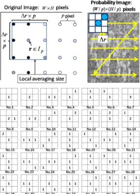
In this study, the grid sampling of local features [2] is carried out at pixel interval of p for simplicity. We denote the set of sample points as Ip
and the map of (pseudo) posterior probability of the codebook of each local region as a posterior probability image. Examples of posterior probability images are shown in Fig. 1. White color represents the high probability. The
Figure 1: Posterior probability images (Bayes’ theorem): Original image, posterior prob-ability of BIKE (left), posterior probprob-ability of CAR (middle), and posterior probprob-ability of PEOPLE (right). These posterior probability images are calculated by using a two-pixel interval (p = 2); for easy understanding, the original images are resized to the size of the posterior probability images. The actual size of the original images are larger than the posterior probability images by p×p pixels. Local features and the codebook are the same as those used in experiment (Sec. 4.1).
data are obtained from the IG02 dataset used in the following experiment (Sec. 4.1). The dataset contains three categories, namely, BIKE, CAR, and PEOPLE. It is observed that the human-like contours appear in the posterior probability image of the PEOPLE category. Thus, the posterior probability images contain some spatial information about the category.
3.2. PHLAC
Autocorrelation is defined as the product of signal values from different points and represents the strong co-occurrence of these points. Higher-order local autocorrelation (HLAC) [11] has been proposed for extracting spatial autocorrelations, and its effectiveness has been demonstrated in several ap-plications such as face and texture classification [22]. To capture the spatial
autocorrelations of posterior probability, we define HLAC features of poste-rior probability images in terms of PHLAC. The definition of the Nth order PHLAC is as follows. R(c,a1, ...,aN) = ∫ Ip P(c|VV Q(r))P(c|VV Q(r+a1)) · · ·P(c|VV Q(r+a N))dr. (6)
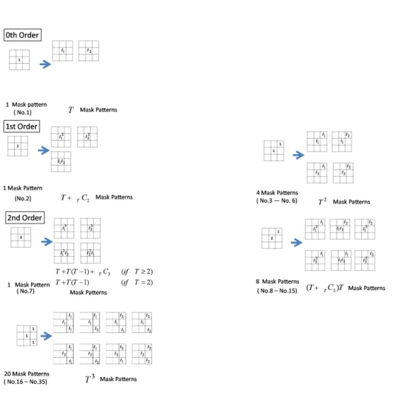
In practice, many forms of Eq. (5) can be obtained by varying the pa-rameters N and an. In this paper, these parameters are restricted to the
following subset: N ∈ {0,1,2} and anx, any ∈ {±∆r×p,0}. By eliminating
duplicates that arise from shifts of center positions, the mask patterns of PHLAC can be represented as shown in Fig. 2. These mask patterns are the same as the 35 HLAC mask patterns [11]. Thus, PHLAC inherits the desirable properties of HLAC for object recognition, namely, shift invariance and additivity. Although PHLAC does not exhibit scale invariance, it can be realized by using several sizes of mask patterns and local features that exhibit scale invariance.
By calculating the correlations in local regions, PHLAC becomes robust against small spatial difference and noise. These local regions can be pre-processed by calculating their values in terms of various alternatives such as their max, average, or median. We found that the optimum alternative is the average. Thus, the practical formulation of PHLAC is given by
0thorder RN=0(c) = ∑ r∈Ip La(P(c|VV Q(r))) (7) 1storder RN=1(c,a1) = ∑ r∈Ip La(P(c|VV Q(r)))La(P(c|VV Q(r +a1))) 2ndorder RN=2(c,a1,a2) = ∑ r∈Ip La(P(c|VV Q(r)))La(P(c|VV Q(r +a1)))
Algorithm 1. PHLAC computation
Training Image:
1) Create codebooks by using local features and a clustering algorithm. 2) Configure posterior probability of each codebook.
Training and Test Image:
3) Create C posterior probability images by using ppixel intervals. 4) Preprocess posterior probability images (local averaging).
5) Calculate HLAC features on posterior probability images by sliding HLAC mask patterns.
La(P(c|VV Q(r +a2))),
where La represents the local averaging on a (∆r ×p)×(∆r ×p) region
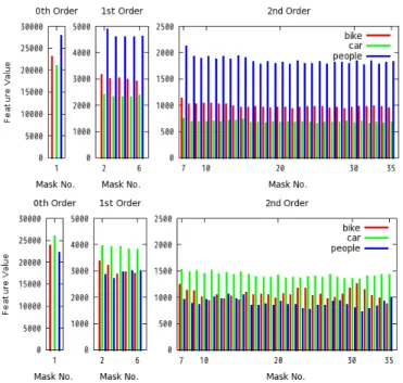
centered on r (Fig. 2). PHLAC is obtained by calculating the HLAC on local-averaged posterior probability images (see Algorithm 1). PHLAC is extracted from the posterior probability images of all categories; thus the total number of features of PHLAC becomes 35×C. Examples of PHLAC feature vector are shown in Fig. 3. It is noticed that difference in the feature values of each category is prominent, and some patterns that are different from the 0th order appear in the higher-order feature values. There are two possibilities with regard to the classification using PHLAC image representations. One is the classification using all PHLACs of all categories (PHLAC.All), and the other is using the PHLAC of one category for each one-against-all classifiers (PHLAC.Clw). We compare these classification methods in the following experiments (Sec. 4.1.1).
Figure 2: PHLAC: local averaging size (left), extracting process (right) and mask patterns (bottom). The numbers {1,2,3} of the mask patterns show the frequency at which their pixel value is used for obtaining the product expressed in Eq. (6).
3.3. Interpretation of PHLAC
Bag of features (0th) + local autocorrelations (1st + 2nd) : If we use SVM weights as pseudo probabilities, then the 0th order of the PHLAC be-comes the same as that obtained during the classification by the standard bag-of-features method using linear SVM. BecauseHis a histogram (see Eq. (2)), Eq. (3) is rewritten as follows.
argmax c∈C{ K ∑ k=1 αc,V Q(rk)+bc} (8)
Figure 3: Examples of PHLAC feature vector. The values ∆r= 48 and p = 2 is used for the images shown in Fig. 1. Original images are those of PEOPLE (top), CAR (bottom).
=argmax c∈C{ K ∑ k=1 (αc,V Q(rk)−min{αc}) +Kmin{αc}+bc} (9) =argmax c∈C{AcRN=0(c) +Bc}, (10) where Ac = ∑M
m=1(αc,m−min{αc}) andBc =Kmin{αc}+bc. (To achieve
the transformation from Eq. (8) to Eq. (9), the relationship RN=0(c) =
∑K
k=1
αc,V Q(rk)−min{αc}
Ac is used.) It can be inferred from this equation that
the classification by the standard bag-of-features method is possible only by using 0th order of the PHLAC and learned parameters Ac and Bc. (It was
assumed that preprocessing was not carried out in the calculation of PHLAC ). In this case, the SVM weight is used as the pseudo posterior probability; however, it is expected that other posterior probabilities may also posses
a similar property of the 0th order PHLAC. Because the histogram of the standard bag of features is created without using local co-occurrences, the 0th order of PHLAC is almost thought of as a one-against-all bag-of-features classification. Higher-order features of PHLAC have richer information on posterior probability images (e.g., the shape of local posterior probability dis-tributions). Thus, if any commonly existing patterns are contained in specific classes, this representation can be expected to achieve better classification performance than the standard bag-of-features method.
The relationship between the standard bag-of-features method and PHLAC classification is shown in Fig. 4. In our PHLAC classification, we train an additional classifier using the 0th order PHLAC{RN=0(1), ...,RN=0(C)}and
use the higher-order PHLAC as a feature vector. In following experiment (Sec. 4.1.1), the classifier is also trained when only the 0th order PHLAC is used. Thus, only the 0th order PHLAC can possibly perform better than the standard bag-of-features method.
Synonymy invariance : Synonymous codebooks are codebooks that have similar posterior probabilities [5]. PHLAC classification can be carried out directly on the posterior probability images, and the same features can be extracted even when a local appearance of an image is exchanged with other appearances whose posterior probabilities are the same as the local appear-ance. This synonymy invariance is important for creating compact image representations [12].
3.4. MFPHLAC
Recently, it has been reported that high classification performance can be achieved by implementing methods that use multiple local features in
Figure 4: Schematic comparison of the standard bag-of-features classification with our proposed PHLAC classification.
generic object recognition problems [23, 24]. Although PHLAC can be cal-culated from posterior probability images estimated by several features in-dependently, it is expected that richer information can be extracted by au-tocorrelations of posterior probability by using multiple features. We extend PHLAC to autocorrelations of posterior probability calculated from multiple image features. We call this image representation method as MFPHLAC.
Assuming that we use T (T≥ 2) types of local features, the definition of the Nth order MFPHLAC can be expressed as follows.
R(c, t0, ..., tNa1, ...,aN) =
∫
Ip
Pt0(c|VV Q(r))Pt1(c|VV Q(r+a1))
· · ·PtN(c|VV Q(r +aN))dr. (11)
Here Pt indicates the posterior probability estimated by feature type t∈
{1, ..., T}.
As in the case with PHLAC, the parameters N and an are restricted to
practical formulation of MFPHALC is given by 0thorder RN=0(c, t0) = ∑ r∈Ip La(Pt0(c|VV Q(r))) (12) 1storder RN=1(c, t0, t1.a1) = ∑ r∈Ip La(Pt0(c|VV Q(r)))La(Pt1(c|VV Q(r +a1))) 2ndorder RN=2(c, t0, t1, t2,a1,a2) = ∑ r∈Ip La(Pt0(c|VV Q(r)))La(Pt1(c|VV Q(r +a1)))La(Pt2(c|VV Q(r+a2))).
Here, MFPHLAC is calculated by sliding extended mask patterns from PHLAC (Algorithm 2). By eliminating duplicates that arise from the second and third power of a certain pixel, the mask patterns of MFPHLAC can be represented as shown in Fig. 5. In Fig. 5, the mask pattern with two features is shown. The independent number of feature values that arise from the second power of a certain pixel isT+TC2, because there existT combinations of the second
power of the same features and TC2 combinations obtained by the
multipli-cation of different feature values. For example, the number of mask patterns become 233 whenT = 2 and 739 whenT = 3. Since MFPHLAC involves the calculation of autocorrelation from multiple features, these features contain richer information than PHLAC features calculated from multiple features independently. Thus, it is expected that better classification performance can be achieved by using MFPHLAC.
4. Experiment
We compared the classification performances of the standard bag-of-features method and PHLAC using three commonly used image datasets:
Algorithm 2. MFPHLAC computation
Training Image:
1) Create T types of codebooks by using local features and a clustering al-gorithm.
2) Configure T posterior probabilities of each codebook type.
Training and Test Image:
3) Create C×T posterior probability images by usingp pixel intervals. 4) Preprocess posterior probability images (local averaging).
5) Calculate MFPHLAC on posterior probability images by sliding MF-PHLAC mask patterns.
IG02 [25], a dataset having 15 natural scene categories [2], and Caltech101 dataset [32].
To obtain reliable results, we repeated the experiment 10 times except for Caltech101 dataset. Ten random subsets were selected from the data to create 10 pairs of training and test data. For each of these pairs, a codebook was created by using k-means clustering on the training set. For classification, a linear one-against-all SVM was used. For the implementation of SVM, we used LIBSVM. Five-fold cross validation was carried out on the training set to tune the parameters of SVM. The classification rate reported by us is the average of the per-class recognition rates, which in turn are averaged over 10 random test sets. With regard to Caltech101 dataset, we repeated the experiment 5 times.
As local features, we used a SIFT descriptor [26] sampled on a regular grid. The modification by the dominant orientation was not used and the descriptor was computed on a 16×16 pixel patch sampled every 8 pixels
Figure 5: Mask patterns of MFPHLAC(In the case of 2 features (t1, t2)).
(p= 8). In the codebook creation process, all the features sampled every 16 pixels on all training images were used for k-means clustering. We used the L2-norm normalization method for both the standard bag-of-features method and PHLAC. In PHLAC, the features were L2 normalized by each order of autocorrelations. We denote the classification of PHLAC using posterior probability by Bayes’ theorem as PHLACBayes and PHLAC using pseudo
al-though the SVM of the standard bag-of-features method is used in Eq. (4) of PHLACSV M, the result of the 0th order PHLACSV M is different from the
result of the standard bag-of-features method because we train an additional linear SVM as mentioned in Sec. 3.3.
4.1. Results of IG02 dataset
4.1.1. Basic property
First, we used the IG02 [25] (INRIA Annotations for Granz-02) dataset, which contains large variations of the target size. The classification task is to classify the test images into 3 categories, i.e., CAR, BIKE, and PEOPLE. The number of training images in each category is 162 for CAR, 177 for BIKE, and 140 for PEOPLE. The number of test images is the same as that of the training images. We resampled 10 sets of training and test sets from all images. The image size was 640×480 pixels or 480×640 pixels. Marasza-lek et al. prepared mask images that indicated the locations of the target objects. We also attempted to estimate the posterior probability of Eq. (1) by using only the local features of the target object region. We denote these PHLAC features as PHLACM ASK. The experimental results are shown in
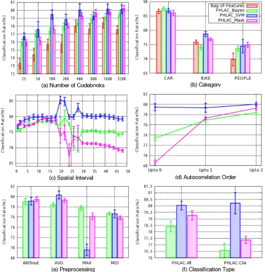
Fig. 6.
Overall performance: The basic settings used were a spatial interval ∆r= 12 and the classification using PHLACs of all categories (PHLAC.All). In all the codebook sizes, all types of PHLACs achieve higher classification perfor-mances than the standard bag-of-features method (Fig. 6(a)). PHLACSV M
achieves higher classification rates than PHLACBayes. By using mask images
for estimating the posterior probability, the performance of PHLACM ASK
Recognition rates per category: The classification rates of PHLAC are higher than those of the standard bag-of-features method in almost all cases (Fig. 6(b)). Especially, the classification rates of the PEOPLE category us-ing PHLAC are higher than those usus-ing the standard bag-of-features method for any settings of PHLAC. This is because human-like contours (shown in Fig. 1) appear in the posterior probability images obtained from images of PEOPLE; these contours were less visible in the posterior probability images obtained from images of other categories.
Spatial interval: The spatial interval appears to be better near ∆r = 12 (12×8 = 96 pixels) for all settings except for PHLACSV M (Fig. 6(c)). The
classification rates of PHLACBayes and PHLACM ASK decrease as the spatial
interval is increased from ∆r= 20. In the case of PHLACSV M, classification
rates are high even when the spatial interval increases, and the peak of the classification rates appears near ∆r = 20. However, at ∆r= 20, the classifi-cation rates for PHLACBayes and PHLACM ASK reduce; therefore, as a basic
settings, we set the spatial interval to ∆r = 12. In practice, a multiscale spatial interval is more useful than a single spatial interval, because there are several optimal spatial intervals (Sec. 4.1.2).
Order of autocorrelation: In the cases of PHLACBayesand PHLACM ASK,
the classification rates increase with the order of autocorrelation (Fig. 6(d)). PHLACSV M exhibit a higher classification performance than other PHLACs
using only 0th order autocorrelations. Thus, the PHLACSV M did not
de-crease the classification performance compared to other PHLACs in the non optimal spatial intervals ( ∆r > 22 ). For experiments using up to 2nd order autocorrelations, PHLACSV M can achieve the best classification
per-formance. Especially in the optimal spatial interval of PHLACSV M (∆r =
20), the classification using the 2nd order autocorrelation was 5.01% better than 0th order autocorrelation (Fig. 6(c)).
Preprocessing: As can be observed from Fig. 6(e), the graphs of the local averaging and no preprocessing cases appear to be comparable. However, when the codebook size and spatial intervals are changed, the local averag-ing often outperformed the no preprocessaverag-ing case. Thus, we recommend the use of local averaging for preprocessing.
Classification type: Of the different classification types, PHLAC.All ex-hibits better performance than PHLAC.Clw (Fig. 6(f)) in PHLACBayes
and PHLACM ASK. On the other hand, when the PHLACSV M is used, the
PHLAC.Clw classification performs better than the PHLAC.All. This indi-cates that the number of dimensions for the training of each SVM can be reduced to 35 when PHLACSV M.
4.1.2. Multiscale spatial interval
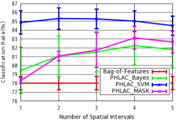
A multiscale spatial interval can capture several spatial co-occurrences. Thus, such an interval is expected to exhibits a higher classification perfor-mance than a single spatial interval, described in the paper cited in [22]. We concatenated the feature vector calculated from different sizes of mask patterns by varying the spatial interval ∆r. We experimented with all combi-nations of ∆r by using the values{2, 4, 8, 16, 22} for each number of spatial intervals. The classification result reported in this paper is the best classi-fication rate selected from the results obtained for these combinations. The classification rates of PHLAC using a multiple spatial interval are shown in Fig. 7. In Fig. 7, PHLAC.All was used. It is confirmed that the performance
of PHLACBayes and PHLACM ASK improved when the number of spatial
in-tervals was increased to four. The use of PHLACSV M does not increase the
accuracy because only ∆r = 22 is higher than other spatial intervals. How-ever, the performance did not decrease when a multiple spatial interval of four was used. These results indicate that the use of a multiscale spatial interval is desirable for both reducing the setting cost of ∆r and improving the classification accuracy.
4.2. Results of Scene-15 dataset
4.2.1. Results of PHLAC
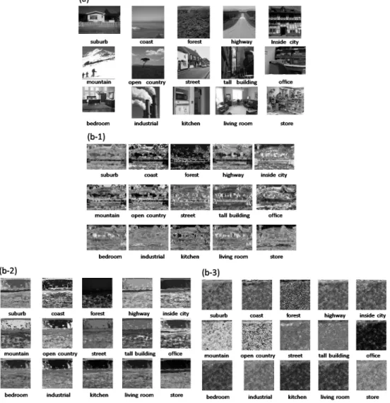
Next, we performed experiments on the 15 dataset [2]. The Scene-15 dataset consists of 4485 images spread over Scene-15 categories. The Scene-15 cat-egories contain 200 to 400 images each and range from natural scenes like mountains and forests to man-made environments like kitchens and offices. We selected 100 random images from each category as a training set and the remaining images as the test set. Some examples of dataset images and posterior probability images are shown in Fig. 10.
We used PHLAC.All, and experimentally set the spatial interval to ∆r = 8. This was determined by comparing the result of ∆r = { 1, 2, 4, 6, 8, 12 } in codebook size 200 (Fig.). The actual size of each mask pattern coressponding to ∆r ={1, 4, 8} are shown in Fig.x . This shows the larger regions correlation produce better performance. However, the minimum size of mask pattern (∆r= 1) already outperformed the standard bag-of-features. The recognition rates for the Scene-15 dataset are shown in Fig. 11. For the Scene-15 dataset, PHLAC achieves higher recognition performances than the standard bag-of-features classification for all categories and
code-book sizes. For this dataset, PHLACBayes exhibits higher accuracy than
PHLACSV M. When the codebook size is 200, the recognition rate of PHLACBayes
is 15% higher than that of the standared bag-of-features classification. In our experiment, the classification rates of PHLACBayes are around
69.48 (±0.27)% by using linear SVM for a codebook size of 200, and that the classification rates of the standard bag-of-features classification using a his-togram intersection kernel [2] are around 66.31 (±0.15)%. Lazebnik reported differences in the 72.2 (±0.6)%; this difference can be attributed to the dif-ferences in the implementations such as feature extraction and codebook creation. The proposed method and the standard bag-of-features method use the same codebook and features used in our experiments.
The examples of PHLACBayes features are shown in Fig. 12. These
ex-amples are of those sex-amples that are classified correctly by PHLACBayes; the
bag-of-features method failed to classify these samples. It is noticed that the posterior probabilities of correct category are not maximum in 0th order; the 1st order feature values of the correct category increase for some samples ( inside city and street ). However, it is not necessary the posterior proba-bilities of correct category are high. We can also use the other categories evidences such as mountain likely contains forest and open country like re-gions in both 0th and higher order feature values for final classifiers. On the basis of all these evidences, the PHLAC classification outperformed the classification carried out using the standard bag-of-features method.
4.2.2. Results of MFPHLAC
Next, we compared MFPHLAC and PHLAC using a multiscale spatial interval. The number of features used simultaneously is restricted to 2 (T
= 2). We use 5 features as local features. These are Intensity, GLAC [15], CS-LBP [27], Texton in addition to the SIFT-like features (S) described in the beginning of Sec. 4.
Intensity (I): A 128-dimensional intensity histogram in a 4×4 cell obtained from a 16×16 pixel patch is used. The intensity level of a pixel is divided to 8 level from the original 0-255 intensity value. L1 normalization is used in each cell.
GLAC (G): A 256-dimensional co-occurrence histogram of gradient di-rection that contains 4 types of local autocorrelation patterns is used. We calculated the feature values from a 16×16 pixel patch, and histogram of each autocorrelation pattern is L2-Hys normalized.
CS-LBP (C): A 256-dimensional histogram of 64 types of intensity pat-terns per 4×4 cells obtained from 16×16 pixel patch is used. We applied L2-Hys normalization to each cell.
Texton (T): The histogram of filter responses in a 16×16 pixel patch is used. We used 13 types of Schmid filters [28] and 8 directions and 3 sizes of the multi resolution Gabor filter [29]. We considered the positive and negative responses of the Schmid filter; thus, the number of dimensions of the filter was 26. We considered the amplitude of the responses of Gabor filter; thus, the dimension of the filter was 24. In total, the number of dimensions of Texton was 50. We applied L2 normalization to each filter type.
For all features, we created 200 codebooks by k-means clustering. In PHLAC and the bag-of-features method using multiple features, the results were obtained by using a concatenated feature vector having multiple feature type. Posterior probability images were created by using Bayes’ theorem.
PHLAC.All was used for the classification method.
We concatenated the feature vector calculated from different sizes of mask patterns, as described in Sec. 4.1.2. We experimented with all combinations of ∆rby using the values{1, 2, 4, 8, 12}for each number of spatial intervals. The classification result reported in this paper is the best classification rate selected from the results obtained for these combinations. Since MFPHLAC requires a large number of dimensions, we restricted the number of the spatial intervals for MFPHLAC to 2. The features of MFPHLAC were L2 normalized by each order of autocorrelations.
It is known that the use of spatial information is very effective [2] in achieving the high accuracy for Scene-15 dataset. We also compared the proposed methods with the bag-of-features using spatial information. Spatial information is realized by spatial binning of an image, and then, a bag-of-features histogram is created in each spatial bin. The setting for the spatial binning are SI1(2×2), SI2(4×4), and PSI(1×1, 2×2, 4×4). The features of the bag-of-features method with spatial information is L2 normalized by each binning setting. These setting of the spatial binning are the same as the setting cited in [2]; however, to compare only the goodness of feature representation, linear SVM is used for all the methods. The results are shown in Fig. 13.
In all features, PHLAC achieved a considerably higher classification formance than the standard bag-of-features method. The classification per-formance improves better as the number of multiple spatial intervals in-creases. MFPHLAC achieved better performance than PHLAC for the same number of multiple spatial intervals. PHLAC performs slightly better than
the spatial pyramid bag-of-features method with a single feature. The per-formance of MFPHLAC and PHLAC are competitive compared to that of the spatial pyramid bag-of-features method with two features.
4.3. Results of Caltech101 dataset
Finaly, we compared PHLAC and BOF using Caltech101 dataset [32]. The Caltech101 dataset contains 8677 images spread over 101 object cate-gories, where the number of images in each category varies from 31 to 800 images. We used 30 images for training per category, and 50 images per category were used for testing. We report the random selection 5 times and report the average classification accuracy. Becuase the image size differs per image in this dataset, we resized the original images so that the all im-ages have almost the same pixels ( z × z pixels). To extract three sizes of local feature, we use three image size z and we changed the sampling in-terval of feature becuase the large size for correspinding image size so that (z, p) ∈ (100,2),(200,4),(400,8). In this set up, we used PHLAC.All and PHLAC.Bayes, and experimentaly set the spatial interval to ∆r = 8 for all image sizes. The recognition features was concatenated feature of three size of original features with regard to both bag-of-features and PHLAC. As local features, we used SIFT-like feature and following OpponentSIFT features[31]. OppnentSIFT(Opp): The rgb color space is converted to opponent color space. Then calculate SIFT-like feature over the all opponent color spaces, independently. This gives 3×128 dimensional feature. We applied L2-Hys normalization to each color space.
We used 400 codebooks created by k-means clustering. The reuslts are shown in Fig. 14. In this dataset, the PHLAC achieved also better
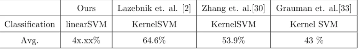
perfor-Table 1: Comparison of other method on the Caltech101
Ours Lazebnik et. al. [2] Zhang et. al.[30] Grauman et. al.[33] Classification linearSVM KernelSVM KernelSVM Kernel SVM
Avg. 4x.xx% 64.6% 53.9% 43 %
mances both SIFT-like and OpponentSIFT features were used for local fea-tures. SIFT-like feature exhibited better performance than OpponentSIFT. The method achieved 4x.x % average recognition rate. The comparison to other recent proposed method in the same setting is shown in table 1. Our recognition rate is less than that of other methods because the classifica-tion rule is so simple. Despite the linear classificaclassifica-tion, the method acheived comparable results to that of Grauman et. al. [33].
5. Discussion on feature dimension
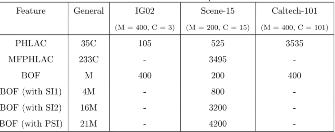
One of the advantages of PHLAC is its feature dimension. The compari-son of the dimension of different feature representation are listed in Table 2. The dimension of the bag-of-features method depends on the codebook size M. Thus, to achieve high accuracy, the training time of a classifier should be increased and a large memory size is required. Furthermore, it is necessary for larger dimensions to utilize spatial grid information. On the other hand, the dimension of PHLAC depends on the number of categories C, and it is independent of the codebook size M. At least, the 0th order of PHLAC can reflect the reliable estimation of large codebook size; thus, the accu-racy of PHLAC can be increased by not increasing the feature dimension. PHLACSV M must train SVM using bag-of-features for estimations posterior
dataset which contains large number of category compared to PHLACBayes.
Thus, we highly recommend the use of PHLAC using Bayes’ theorem when the codebook size and number of categories are large. Although it is obvious that the dimension of PHLAC for all categories becomes large for a prob-lem which involving a very large number of categories, the number of the category that is classified once undergoes reduction by hierarchal category recognition.
Furthermore, the PHLAC feature can be compressed effectively by prin-ciple component analysis (PCA). The recognition rates per compressed di-mension by PCA are shown in Fig. 15. In this experiment, PHLACBayes and
PHLAC.All were used. Because redundancy exists owing to similar prop-erties of mask patterns and similar posterior probability images of different categories, the performances do not decrease even when the dimension is less than 40% of the original PHLAC dimension. Thus, the feature dimension of PHLAC can be further reduced from linear size of the categories with maintaining the classification accuracy.
Table 2: Dimensions of feature representations
Feature General IG02 Scene-15 Caltech-101
(M = 400, C = 3) (M = 200, C = 15) (M = 400, C = 101)
PHLAC 35C 105 525 3535
MFPHLAC 233C - 3495
-BOF M 400 200 400
BOF (with SI1) 4M - 800 -BOF (with SI2) 16M - 3200 -BOF (with PSI) 21M - 4200
-6. Conclusion
In this paper, we proposed an image description method using higher-order local autocorrelations on posterior probability images called “probabil-ity higher-order local autocorrelations (PHLAC).” This method is regarded as an extension of the standard bag-of-features method. Our method over-comes the limitation of spatial information by utilizing the co-occurrence of local spatial patterns in posterior probabilities. This method possesses the properties of shift invariance and additivity as does HLAC [11]. Experimen-tal results revealed that the proposed method achieved a higher classification performance than the standard bag-of-features method by an average of 2% and 15% in the case of the IG02 and Scene-15 datasets, respectively, using 200 codebooks. In Caltech-101, the proposed method improved x% using 400 codebooks. We also extended PHLAC to autocorrelations of posterior probability calculated from multiple image features, which is called “mul-tiple features probability higher-order local autocorrelations (MFPHLAC).” MFPHLAC was able to achieve a slightly better performance than PHLAC. We also compared the proposed methods with the bag-of-features method using spatial information. PHLAC was able to achieve a competitive result compared to the bag-of-features method using spatial information.
References
[1] G.Csurka, C.R.Dance, L.Fan, J.Willamowski, C.Bray, Visual catego-rization with bag of keypoints, in: European Conference on Computer Vision, Workshop on Statistical Learning in Computer Vision, 2004, pp.59–74.
[2] S.Lazebnik, C.Schmid, J.Ponce, Beyond bags of features: spatial pyra-mid matching for recognizing natural scene categories, in: IEEE Con-ference on Computer Vision and Pattern Recognition, 2006, pp.2169– 2178.
[3] A.Agarwal, B.Triggs, Multilevel Image coding with hyperfeatures, In-ternational Journal of Computer Vision 78 (2008) 15–27.
[4] S.Savarse, J.Winn, A.Criminisi, Discriminative object class models of appearance and shape by correlatons, in: IEEE Conference on Com-puter Vision and Pattern Recognition, 2006, pp.2033–2040.
[5] J.Yuan, Y.Wu, M.Yang, Discovery of collocation patterns: from visual words to visual phrases, in: IEEE Conference on Computer Vision and Pattern Recognition, 2007, pp.1–8.
[6] F.Jurie, B.Triggs, Creating efficient codebooks for visual recognition, in: IEEE International Conference on Computer Vision, 2005, vol.1 pp.604–610.
[7] E.Nowak, F.Jurie, B.Triggs, Sampling strategies for bag-of-features im-age classification, in: European Conference on Computer Vision, 2006, pp.490–503.
[8] J.C.V.Gemert, J.-M.Geusebroek, C.J.Veenman, A.W.M.Smeulders, Kernel codebooks for scene classification, in: European Conference on Computer Vision, Part III, LNCS 5304, 2008, pp.696–709.
[9] F.Perronnin, Universal and adapted vocabularies for generic visual cat-egorization, IEEE Transaction on Pattern Analysis and Machine Intel-ligence 30 (7) (2008) 1243–1256.
[10] A.Bosch, A.Zisserman, X.Munoz, Image classification using random forests and ferns, in: IEEE International Conference on Computer Vi-sion, 2007, pp.1–8.
[11] N.Otsu, T.Kurita, A new scheme for practical flexible and intelligent vision systems, in: IAPR Workshop on Computer Vision, 1988, pp.431– 435.
[12] Y.-T. Zheng, M.Zhao, S.-Y.Neo, T.-S.Chua, Q.Tian, Visual synset: towards a higher-level visual representation, in: IEEE Conference on Computer Vision and Pattern Recognition, 2008, pp.1–8.
[13] T.Matsukawa, T.Kurita, Image classification using probability higher-order local auto-correlations, in: Asian Conference on Computer Vi-sion, Part III, LNCS 5996, 2009, pp.384–394.
[14] E.Shechtman, M.Irani, Matching local self-similarities across images and videos, in: IEEE Conference on Computer Vision and Pattern Recognition, 2007, pp.511–518.
[15] T.Kobayashi, N.Otsu, Image feature extraction using gradient local auto-correlations, in: European Conference on Computer Vision, Part I, LNCS 5302, 2008, pp.346–358.
[16] T.Kobayashi, N.Otsu, Color Image feature extraction using color in-dex local auto-correlations, in: International Conference on Acoustics, Speech, and Signal Processing, 2009, pp.1057–1060.
[17] T.Quack, V.Ferrari, B.Leibe, L.Van-Gool, Efficient mining of frequent and distinctive feature configurations, in: IEEE International Confer-ence on Computer Vision, 2007, pp.1–8.
[18] X.Wang, E.Grimson, Spatial latent dirichlet allocation, in: Advances in Neural Information Processing Systems, 2007, vol.20.
[19] N.Rasiwasia, N.Vasconcelos, Scene classification with low-dimensional semantic spaces and weak supervision, in: IEEE Conference on Com-puter Vision and Pattern Recognition, 2008, pp.1–8.
[20] J.Shotton, M.Johnson, R.Cipolla, Semantic texton forests for image categorization and segmentation, in: IEEE Conference on Computer Vision and Pattern Recognition, 2008, pp.1–8.
[21] V.Vapnik, Statistical learning theory, John Wiley & Sones, New York, USA, 1998.
[22] T.Toyoda, O.Hasegawa, Extension of higher order local autocorrelation features, Pattern Recognition 40 (2007) 1466–1473.
[23] M.Varma, D.Ray, Learning the discriminative power-invariance trade-off, in: IEEE International Conference on Computer Vision, 2007, pp.1–8.
[24] A.Bosch, A.Zisserman, X.Munouz, Representing shape with a spatial pyramid kernel, in: International Conference on Image and Video Re-trieval, 2007, pp.401–408.
[25] M.Marszalek, C.Schmid, Spatial weighting for bag-of-features, in: IEEE Conference on Computer Vision and Pattern Recognition, 2006, vol.2 pp.2118–2125.
[26] D.G.Lowe, Distinctive image features from scale-invariant keypoints, International Journal of Computer Vision 60 (2004) 91–110.
[27] M.Heikkila, M.Pietikainen, C.Schmid, Description of interest regions with local binary patterns, Pattern Recognition 42 (2009) 425–436. [28] C.Schmid, Constructing models for content-based image retrieval, in:
IEEE Conference on Computer Vision and Pattern Recognition, 2001, vol.2 pp.39–45.
[29] K.Hotta, Scene classification based on multi-resolution orientation his-togram of gabor features, in: International Conference on Computer Vision Systems, LNCS.vol.5008, 2008, pp.291–301.
[30] J.Zhang, M.Marszalek, S.Lazebnik, C.Schmid, Local features and ker-nels for classification of texture and object categories: a comprehensive study, International Journal of Computer Vision 73(2) (2007) 213–238. [31] K.E.A.van de Sande, T.Gevers, C.G.M.Snoek, Evaluation of color de-scriptors for object and scene recognition, in: IEEE Conference on Computer Vision and Pattern Recognition, 2008, pp.1–8.
[32] L.Fei-Fei, R.Fergus, P.Perona, Learning generative visual models from few training examples: an incremental bayesian approach tested on 101 object categories, in: IEEE CVPR Workshop on Generative-Model Based Vision, 2004.
[33] K.Grauman, T.Darrell, Pyramid match kernels: Discriminative clas-sification with sets of image features, in: International Conference on Computer Vision, Vo.2, pp.1458–1465.
Figure 6: Recognition rates of IG02. The basic settings are codebook size = 400 ((b)–(f)), spatial interval ∆r= 12 ((a),(b),(d)–(f)), and PHLAC.All ((a)–(e)).
Figure 8: Examples of Scene-15 dataset. Examples of the original images (a) and prob-ability images (b). The original images of (b) are suburb (b-1), coast (b-2), and forest (b-3).
Figure 9: Recognition rates of Scene 15 per spatial interval (codebook size is 200).
Figure 10: Actual size of mask patterns. (a): original image, (b): probability image, (c): mask pattern of ∆r= 1, (d): mask pattern of ∆r= 4, (e): mask pattern of ∆r= 8, where green points of (a) is the sampling points of local features and gray areas of (c)-(e) show the local averaged areas.
Figure 11: Recognition rates of Scene 15 per codebook size (left) and per category (right) when codebook size is 200.
Figure 12: Examples of PHLAC features (PHLACBayes); All examples are those of the
samples that were recognized correctly by PHLAC and not recognized by the bag-of-features method.
Figure 13: Recognition rates of MFPHLAC and comparison with those of bag-of-features method with spatial information (Scene-15). SI1 (Spatial Information 2×2), SI2 (Spatial Information 4×4), PSI (Pyramid Spatial Information (1×1, 2×2, 4×4))
Figure 14: Recognition rates of Caltech101
Figure 15: Recognition rates of compressed PHLAC by PCA (Scene-15 dataset): the points of the extreme right indicate original PHLAC without PCA.