1 Introduction. 1.1 Selecting Pizza Toppings

(1)

1

Introduction

In this chapter we introduce the motivation for studying Cognition and Intractability. We provide an intuitive introduction to the problem of intractabil-ity as it arises for models of cognition using an illustrative everyday problem as running example: selecting toppings on a pizza. Next, we review relevant back-ground information about the conceptual foundations of cognitive explanation, computability, and tractability. At the end of this chapter the reader should have a good understanding of the conceptual foundations of the Tractable Cognition thesis, including its variants: TheP-Cognition thesis and the FPT-Cognition thesis, which motivates diving into the technical concepts and proof techniques covered in Chapters 2–7.

1.1

Selecting Pizza Toppings

Imagine you enter a pizzeria to buy a pizza. You can choose any combination of toppings from a given set, e.g., {pepperoni, salami, ham,mushroom,pineapple, . . .}. What will you choose?

According to one account of human decision-making, your choice will be such that you maximize utility. Here utility, denoted byu(.), is to be understood as the subjective value of each possible choice option (e.g., if you prefer salami to ham, then u(salami) > u(ham)). Since you can choose combinations of toppings, we need to think of the choice options as subsets of the set of all available toppings. This includes subsets with only one element (e.g.,{salami} or{olives}), but also combinations of multiple toppings (e.g.,{ham,pineapple} or {salami,mushrooms,olives}). On this account of human decision-making, we can formally describe your toppings selection problem as an instance of the following computational problem:

Generalized Subset Choice

Input: A set X = {x1,x2,...,xn} of n available items and a value

functionuassigning a value to every subsetS⊆X.

Output:A subsetS⊆Xsuch thatu(S) is maximized over all possible S⊆X.

(2)

Note that many other choice problems that one may encounter in everyday life can be cast in this way, ranging from inviting a subset of friends to a party or buying groceries in the grocery store to selecting people for a committee or prescribing combinations of medicine to a patient.

But how – using what algorithm – could your brain come to select a subset S with maximum utility? A conceivable algorithm could be the following: Consider each possible subsetS⊆X, in serial or parallel (in whatever way we may think the brain implements such an algorithm), and select the one that has the highest utilityu(S). Conceptually this is a straightforward procedure. But it has an important problem. The number of possible subsets grows exponentially with the number of items inX. Given that in real-world situations one cannot generally assume thatXis small, the algorithm will be searching prohibitively large search spaces.

Stop and Think

These days pizzerias may provide for 30 or more different toppings. How many distinct pizzas do you think can be made with 30 different pizza toppings?

If n denotes the number of items in X, then 2n expresses the number of distinct possible subsets of X. In other words, with 30 toppings one can make 230 > 1,000,000,000 (a billion) distinct pizzas. Of course, in practice pizzerias typically list 20–30 distinct pizzas on their menus. But consider that some pizzerias also provide the option to construct your own pizza, implicitly allowing a customer to pick any of the billion pizza options available.

Stop and Think

Imagine that the brain would use the exhaustive algorithm described earlier for selecting the preferred pizza. Assume that the brain’s algo-rithm would process 100 possible combinations, in serial or parallel, per second. How long would it take the brain to select a pizza if it could choose from 30 different pizza toppings? What if it could choose from 40 different toppings?

You may be surprised to find that the answer is 4 months. That is the time it takes in this scenario for your brain to consider all the distinct pizzas that can be made with 30 toppings in order to find the best tasting one (maximum utility). If the choice would be from 40 toppings, it would even take 3.5 centuries. Evidently, this is an unrealistic scenario. The pizzeria would be long closed before you would have made up your mind!

(3)

1.1 Selecting Pizza Toppings 5

There is an important lesson to draw from our pizza example: Explaining how agents (human or artificial) can make decisions in the real world, where time is a costly resource and choice options can be plentiful, requires algorithms that run in a realistic amount of time. The exhaustive algorithm that we considered in our pizza scenario does not meet this criterion. It is an exponential-time algorithm. The time it takes grows exponentially with the input size n (i.e., grows ascn for some constant c > 1). Exponential time grows faster than any polynomial function (a function of the formnc_{for some}

constantc), and is therefore also referred to as non-polynomial time. Another example of non-polynomial time is factorial time (grows asn!). An example of a factorial-time algorithm would be an algorithm that exhaustively searches all possible orderings ofnevents or actions in order to select the best possible ordering. Consider, for instance, planning nactivities in a day: going to the hairdresser, doing the laundry, buying groceries, cooking food, washing the dishes, posting a letter, answering an email, watching TV, etc. Even for as few as 10 activities, there would be 3.6 million possible orderings, and for 20 activities there would be more than 1018 possible orderings. Planning one’s daily activities by exhaustive search would be as implausible as selecting pizza toppings by exhaustive search.

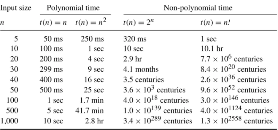
Table 1.1 illustrates why non-polynomial time (e.g., exponential or factorial) algorithms generally are consideredintractablefor all but small input sizesn, whereas polynomial-time algorithms (e.g., linear or quadratic) are considered tractable even for larger input sizes. Informally, intractable means that the

Table 1.1 Illustration of the running times of polynomial time versus super-polynomial time algorithms. The functiont(n)expresses the number of steps performed by an algorithm (linear, quadratic, exponential, or factorial). For illustrative purposes it is assumed that 100 steps can be performed per second.

Input size Polynomial time Non-polynomial time n t(n)=n t(n)=n2 t(n)=2n t(n)=n!

5 50 ms 250 ms 320 ms 1 sec

10 100 ms 1 sec 10 sec 10.1 hr

20 200 ms 4 sec 2.9 hr 7.7×106centuries

30 299 ms 9 sec 4.1 months 8.4×1020centuries

40 400 ms 16 sec 3.5 centuries 2.6×1036centuries 50 500 ms 25 sec 3.6×103centuries 9.6×1052centuries 100 1 sec 1.7 min 4.0×1018centuries 3.0×10146centuries 500 5 sec 41.7 min 1.0×10139centuries 4.0×101124centuries 1,000 10 sec 2.8 hr 3.4×10289centuries 1.3×102558centuries

(4)

algorithm requires an unrealistic amount of computational resources (in this case, time) for its completion. This intractability is the main topic of this book. In this book we explore formal notions of (in)tractability to assess the computational-resource demands of different (potentially competing) scientific accounts of cognition, be they about decision-making, planning, perception, categorization, reasoning, learning, etc. Even though brains are quite remark-able, their speed of operation is limited, and this fact can be exploited to assess the plausibility of different ideas scientists may have about “what” and “how” the brain computes.

For illustrative purposes, Table 1.1 assumed that the listed algorithms could perform 100 steps per second. To see that this assumption has little effect on the large difference between polynomial and non-polynomial running times perform the next practice.

Practice 1.1.1 Recompute the contents of Table 1.1 under the assumption

that the algorithms can perform as many as 1,000 steps per second.

Let us return to our pizza example. We saw that the exhaustive algorithm (searching all possible subsets) to maximize utility of the chosen subset of toppings is an intractable algorithm. Does this mean that the idea that humans maximize utility in such a situation is false? Possibly, but not necessarily. Note that the trouble may have arisen from the specific way in which we formalized the maximum utility account of decision-making for subset choice. In the Generalized Subset Choice problem we allowed for any possible utility functionuthat assigned any possible value to every subsetX. As a result, there is only one way to be sure that we output a subset with maximum utility: We need to consider each and every subset.

The situation would be less dire if somehow there would be regularity in one’s preferences over pizza toppings. This regularity could then perhaps be exploited to more efficiently search the space of choice options. For instance, if subjective preferences would be structured such that the utility of a subset could be expressed as the sum of the value of its elements (i.e.,u(S)=_x_∈_Su(x)), then we could change the formalization as follows:

Additive Subset Choice

Input: A set X = {x1,x2,...,xn} of n available items and a value

functionuassigning a value to every elementx∈X.

Output:A subsetS ⊆Xsuch thatu(S) =_x_∈_Su(x) is maximized over all possibleS⊆X.

If the pizza selection problem would be an instance of this formal problem, then the brain could select a maximum utility subset by using the following

(5)

1.1 Selecting Pizza Toppings 7

simple linear-time algorithm: Consider each itemx ∈X, and ifu(x)≥0 then addxto the subsetS, otherwise discard the optionx. Since each item inXhas to be considered only once, and the inequalityu(x)≥0 checked for each item only once, the number of steps performed by this algorithm grows at worst linearly with the number of options inX. As can be seen in Table 1.1, such a linear-time algorithm is clearly tractable in practice, even when you have larger numbers of toppings to choose from.

The maximum utility account of decision-making would thus be saved from intractability, if indeed real-world subset choice problems could all be cast as instances of the Additive Subset Choice problem. But is this a plausible possibility?

Stop and Think

Consider selecting pizza toppings for your pizza using the linear-time algorithm described earlier? Why may you not be happy with the actual result?

If you would use the linear-time algorithm to select your pizza top-pings, you would always end up with all positive valued toppings on your pizza. Besides that this may make for an overcrowded pizza, it also fails to take into account that you may like some toppings individually but not in particular combinations. For instance, each of the items in the set {pepperoni,salami,ham,mushroom,pineapple} could have individually posi-tive value for you, in the sense that you would prefer a pizza with any one of them individually over a pizza with no toppings. Yet, at the same time, you may prefer{ham,pineapple}or{salami,mushrooms,olives}over a pizza will all the toppings (e.g., because you dislike the taste of the combination of pineapple with olives). In other words, in real-world subset choice problems, there may be interactions between items that affect the utility of their combinations. This makesu(S) =_x_∈_Su(x) an invalid assumption. From this exploration, we should learn an important lesson: Intractable formalizations of cognitive problems (decision-making, planning, reasoning, etc.) can be recast into tractable formalizations by introducing additional constraints on the input domains. Yet, it is important to make sure that those constraints do not make the new formalization too simplistic and unable to model real-world problem situations.

A balance may be struck by introducing the idea of pair-wise interactions between k items in the choice set. Then we can adapt the formalization as follows:

(6)

Binary Subset Choice

Input:A setX = {x1,x2,...,xn}ofnavailable items. For every item

x ∈ X there is an associated valueu(x), and for every pair of items (xi,xj) there is an associated valueδ(xi,xj).

Output: A subset S ⊆ X, such that u(S) = _x_∈_Su(x) +

x,y∈Sδ(x,y) is maximum.

If situations allow for three-way interactions, this model may also fail as a computational account of subset choice. It is certainly conceivable that three-way interactions can occur in practice (see, e.g., van Rooij, Stege, and Kadlec, 2005). Leaving that discussion for another day, we may ask ourselves the following question: Would computing thisBinary Subset Choice problem be in principle tractable? It is not so easy to tell as forGeneralized Subset Choice, because the utility function is constrained. But is it constrained enough to yield tractability of this computation? Probably not. Using the tools that you will learn about in this book, you will be able to show that this problem belongs to class of so-calledNP-hard problems. This is the class of problems for which no polynomial-time algorithms exist unless a widely conjectured inequality P = NP would be false. This P = NP conjecture, although formally unproven (and perhaps even unprovable), is widely believed to be true among computer scientists and cognitive scientists alike (see Chapter 4 for more details). Likewise, we will adopt this conjecture in the remainder of this book.

1.2

Conceptual Foundations

In our pizza example we have introduced many of the key scientific concepts on which this book builds. For instance, we used the distinction made in cognitive science between explaining the “what” and the “how” of cognition, the notion of “algorithm” as agreed upon by computer scientists, and the idea that “intractability” can be characterized in terms of the time complexity of algorithms. In this section, we explain the conceptual foundations of these concepts in a bit more detail.

1.2.1

Conceptual Foundations of Cognitive Explanation

One of the primary aims of cognitive science is to explain human cognitive capacities. Ultimately, the goal is to answer questions such as: How do humans make decisions? How do they learn language, concepts, and categories? How

(7)

1.2 Conceptual Foundations 9

do they form beliefs, based on reasons or otherwise? In order to come up with answers for such “how”-questions it can be useful to first answer “what”-questions: What is decision-making? What is language learning? What is categorization? What is belief fixation? What is reasoning?

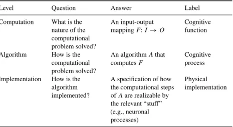
This distinction between “what is being computed” (theinput-output map-ping) and “how it is computed” (the algorithm) is also reflected in the influential and widely used explanatory framework proposed by David Marr (1981). Marr proposed that, ideally, theories in cognitive science should explain the workings of a cognitive system (whether natural or artificial) on three different levels (see Table 1.2). The first level, called thecomputational level, specifies the nature of the input-output mapping that is computed (we will also refer to this as thecognitive function).1The second level, the algorithmic level, specifies the nature of the algorithmic process by which the computation described at the computational level is performed (cognitive process). The third and final level, the implementation level, specifies how the algorithm defined at the second level is physically implemented by the “hardware” of the system (or “wetware” in the case of the brain) performing the computation (physical implementationof the cognitive process/function).

Hence, in David Marr’s terminology, the description of a cognitive system in terms of the function that it computes (or problem that it solves)2is called a computational-level theory. We already saw examples when we discussed the pizza example: i.e., Generalized, Additive, and Binary Subset Choice were three different candidate computational-level theories of how humans choose subsets of options. Since one and the same function can be computed by

1 _{We should note that Marr also intended the computational-level analysis to include an account}

of “why” the cognitive function is the appropriate function for the system to compute, given its goals and environment of operation. This idea has been used to argue for certain

computational-level explanations based on appeals to rationality and/or evolutionary selection – i.e., that specific functions would be rational or adaptive for the system to compute. The intractability analysis of computational-level accounts as pursued in this book are neutral with respect to such normative motivations for specific computational-level accounts, in the sense that tractability and rational analysis are compatible, but the former can be done independent of the latter (see Section 8.5).

2 _{Since the words “function” and “problem” refer to the same type of mathematical object (an}

input-output mapping) we will use the terms interchangeably. A difference between the terms is a matter of perspective: the word “problem” has a more prescriptive connotation of an input-output mapping that is to be realized (i.e., a problem is to be solved), while the word “function” has a more descriptive connotation of an input-output that is being realized (i.e., a function is computed). The reader may notice that we will tend to adopt the convention of speaking of “problems” whenever we discuss computational complexity concepts and methods from computer science (e.g., in Chapters 2–7), and adopt the terms “function” or

“computational-level theory” in the context of applications and debates in cognitive science (e.g., in Chapters 8–12).

(8)

Table 1.2 Marr’s levels of explanation: What is the type of question asked at each level, what counts as an answer (the explanans), and labels for the thing to be explained (explanandum) per level.

Level Question Answer Label

Computation What is the nature of the computational problem solved? An input-output mappingF:I→O Cognitive function

Algorithm How is the computational problem solved? An algorithmAthat computesF Cognitive process Implementation How is the

algorithm implemented?

A specification of how the computational steps ofAare realizable by the relevant “stuff” (e.g., neuronal processes)

Physical implementation

many different algorithms (e.g., serial or parallel), we can describe a cognitive system at the computational level more or less independently of the algorithmic level. Similarly, since an algorithm can be implemented in many different physical systems (e.g., carbon or silicon), we can describe the algorithmic level more or less independently of physical considerations.

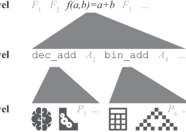
David Marr, in his seminal 1981 book, illustrated this idea with the example of a cash register, i.e., a system that has the ability to perform addition (see Figure 1.1). A computational-level theory for a cash register would be the Addition function F(a,b) = a + b. An algorithmic-level theory could, for instance, be an algorithm operating on decimal numbers or an algorithm operating on binary numbers. Either algorithm would compute the function Addition, albeit in different ways. The implementational-level theory would depend on the physical make-up of the system. For instance, different physical systems can implement algorithms for Addition: cash registers, pocket calculators, and even human brains. An implementational-level theory would specify by some sort of blueprint how the algorithm could be realized by that particular physical system.

Practice 1.2.1 Study the cash-register example in Figure 1.1. Can you come up with different computational-, algorithmic- and implementational-level

(9)

F

₃

f(a,b)=a+b

F

₁

F

₂

...

A

₂

A

₄

...

P

₃

...

P

₆

...

dec_add

bin_add

Computational level

Algorithmic level

Implementational level

Figure 1.1 An illustration of the three levels of analysis by Marr, using Addition.

F

₁

F

₂

F

₃

F

₄

F

₅

F

₆

...

A

₁

A

₂

A

₃

A

₄

A

₅

A

₆

...

P

₁

P

₂

P

₃

P

₄

P

₅

P

₆

...

Computational level

Algorithmic level

Implementational level

Figure 1.2 An illustration of the underdetermination of lower levels of explanation by higher levels of explanation in the Marr hierarchy.

theories for another example? For example, for the pizza topping example or for the example of scheduling activities throughout the day.

Stop and Think

Study the relationship between the levels of Marr in Figure 1.1. Why is it that a given computational-level theory can, in principle, be consistent with different algorithmic-level explanations? And why can a given algorithmic-level explanation be consistent with different implementational-level explanations?

(10)

Note that in Figure 1.2 there is underdetermination of lower-level expla-nations in the Marr hierarchy by higher-level explaexpla-nations. By this we mean that even if a cognitive scientist hypothesizes a particular computational-level theoryF, he or she can remain agnostic about the nature of the exact algorithm Aby which the system under study computesF. What the scientist does need to commit to is that, in principle, there can exist an algorithm that computes F. Similarly, hypothesizing a particular algorithmic-level explanation A for function F, the scientist can remain agnostic about the nature of the exact implementationP,3but she will have to commit to the in principle possibility of realizing and running the algorithm on the relevant hardware or wetware. Figure 1.2 gives the general picture.

David Marr argued for the usefulness of top-down analyses for purposes of reverse engineering natural cognitive systems. The idea of such a top-down approach is that it is best to start by developing a computational-level theory and then work down toward the algorithmic- and implementational-levels theories. He believed this was the best way to make progress in cognitive science, because in his opinion:

an algorithm is likely to be understood more readily by understanding the nature of the problem being solved than by examining the mechanism (and the hardware) in which it is embodied. (Marr, 1981, p. 27; see also Marr, 1977). This book is written to help cognitive scientists interested in adopting this top-down approach by providing useful formal tools for computational-level theory development.4 This is not to say that we think other approaches are not to be pursued as well. In fact, we think that cognitive science can benefit from pluralism in approaches, including bottom-up approaches (starting at the implementational level) and middle-out (starting at the algorithmic level). This book merely aims to add useful formal tools to the cognitive scientist’s toolbox, not to promote one approach over the other.

3 _{We use}_P_for_P_{hysical implementation instead of}_I_for_I_{mplementation to not confuse with our}

notation for inputsI.

4 _{Even theories that are often seen as being formulated at the algorithmic level – such as}

connectionist or neural network models (e.g., McClelland, 2009) – are not free from computational level considerations (Klapper et al., 2018; McClelland, 2009). Also for neural networks it is of interest to study which functions they can and cannot compute (Parberry, 1994). For instance, neural network learning is a computational task: A neural network is assumed to learn a mapping from inputs to outputs by adjusting its connection weights. Here the input of the learning task is given by (I) all network inputs in the training set plus the required network output for each such network input, and the output is given by (O) a setting of connection weights such that the input-output mapping produced by the trained network is satisfactory. This learning task, like any other task in the more symbolic tradition, can be analyzed at the computational level (Blum and Rivest, 1992; Judd, 1990; Parberry, 1994).

(11)

1.2.2

Conceptual Foundations of Computability and Tractability

Given that our focus will be on the top-down approach, it’s vital to realize that there is also another type of underdetermination at play. Namely, the computational-level theory itself is underdetermined by empirical observations (see Figure 1.3). By this we mean that given observations about the behavior of a system one cannot deduce the function that it computes. At best, one can abduce it, i.e., make an inference to the best explanation. The problem of underdetermination of theory by data is not specific, of course, to cognitive science but applies in general to all empirical sciences.

Stop and Think

Consider a system that computes a functionF: I → O, where both I andO denote sets of binary strings. Now imagine you could input different strings to the system and observe for each input the string that the system outputs. Why would this information not be sufficient to deduce the functionF:I →Othat the system is computing?

Coming up with computational-level theories for human cognitive abilities – such as decision-making, categorization, learning, etc. – is a creative scientific process. It is not possible to deduce theories from observations of a system’s behavior for several reasons:

1. Any finite set of input-output observations is consistent with infinitely many different functions.

2. Inputs and outputs are usually not directly observable.

3. Psychological data are noisy (due to context variables not under the control of the experimenter).

4. Commitment is usually to the informal theory, not the specific formaliza-tion.

All four points can be illustrated with our earlier pizza topping example. Let’s say we give a person 20 different sets of toppings to choose from and observe which pizza toppings they choose per set. Then there will be, in principle, multiple set-to-subset functions consistent with the observations, each making a different prediction about what the person would choose if we would make a new, 21st topping, and add that to the set of toppings for them to choose from (point 1 in the previous list). Note, furthermore, that if our computational-level theory is based on the idea that human decision-makers maximize utility, then both the choice options and the final choice set must

(12)

F1 F2 F3 F4 F5 F6 ...

A1 A2 A3 A4 A5 A6 ...

P1 P2 P3 P4 P5 P6 ...

D1

Computational level

Algorithmic level Computability

Tractability Implementational level D2 D3 D4 D5 D6 D7 D8 D9D10 D1 D2 Theory is underdeter-mined by data F1 F2 F3 F4 F5 F6 ? ? ? ? ? ? ? ? ? ? ? ? D3 D4 D5 D6 D7 D8 D9D10 Theory is underdeter-mined by data

Figure 1.3 An illustration of the underdetermination of computational-level theories by data (left) and the lower-level constraints on computational-level theories (right).

have associated utilities. These utilities are aspects of the input and output that are not directly observable; they are a property of the person’s inner mental states, in this case preferences (point 2). Furthermore, even if we would be able to devise procedures to try and estimate those unobservable states, then our measurements would always have some noise and measurement errors that we cannot fully control as scientists. Hence, if the observed behavior of the person would not match exactly with the predictions made by our theory we do not know for sure that it is the theory that is incorrect or that we may have misestimated the person’s utilities (point 3). Lastly, even if based on the noisy and partial input-output observations so far, we would be able to rule out some particular Subset Choice functions that may not be sufficient to falsify the idea that human decision-makers are utility maximizers, because there could exist functions based on alternative formalizations of this informal idea that could be consistent with the observations made to date (point 4).

It seems, thus, that it would be useful if cognitive scientists could appeal to some theoretical constraints on the type of computational-level theories they could come up with. If we reconsider the Marr hierarchy we can see that indeed such constraints are available. Namely, a cognitive scientist postulating a particular F as a candidate hypothesis for the “what” of some aspect of cognition is committing that there exists some physically feasible “how”-answer. In other words, the function should be computable and tractable – computable, because there should be at least one algorithmAthat can compute F; andtractable, because it must be possible to runAusing a realistic amount of resources (time and space) on a physical mechanismP. We will refer to the first requirement as the “computability constraint” and the second requirement as the “tractability constraint” (see Figure 1.3).

In order to be able to assess which functions meet the computability constraint, a precise definition of computationis required. Informally, when

(13)

we say a system computes a function or solves a problem, F: I → O, we mean to say that the system reliably transforms everyi∈I intoF(i)∈Oin a way that can be described by an algorithm. An algorithm is a step-by-step finite procedure that can be performed, by a human or machine, without the need for any insight, just by following the steps as specified by the algorithm.

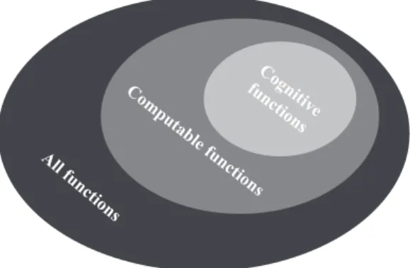
In 1936, Alan Turing presented his machine formalization as a way of making the intuitive notions of “computation” and “algorithm” precise. Turing proposed that every function for which there is an algorithm – which is intuitively computable – is computable by a Turing machine (for more details on this machine formalization we refer the reader to Appendix A). In other words, functions that are not computable by a Turing machine are not computable in principle by any machine. To support his thesis, Turing showed that his formalization is equivalent to a different formalization (λ-calculus), which was independently proposed by Church (1936). The thesis that both Turing’s and Church’s respective formalizations capture the intuitive notion of algorithm is now known as the Church-Turing thesis. Further, Turing’s and Church’s formalizations have also been shown equivalent to all other accepted formalizations of computation (such as based on neural networks, cellular automata, and even quantum computers), by which the thesis has gained more support.5 The Church-Turing thesis has a direct implication for cognitive science: Computational-level theories of cognitive abilities are theoretically constrained to be Turing-computable functions (see Figure 1.4).

Even though the computability constraint can help rule our computationally infeasible computational-level theories, for practical purposes it seems like a too liberal constraint. For instance, we saw that Generalized Subset Choice could be computed by an exhaustive search algorithm, hence the problem is computable. Yet, such an algorithm seems to be intractable. Here, like computability before Turing and others’ formalization of the term, the term “intractability” is an informal notion in need of formalization if we are going to use it to constrain computational-level theories. In this book we will pursue two possible formalizations of tractability: one grounded in what is known as classical complexity theory and one grounded in what is known as parameterized complexity theory.

5 _{Note that the Church-Turing thesis is not a mathematical conjecture that can be proven right or}

wrong. Instead the Church-Turing thesis is a hypothesis about the state of the world. Even though we cannot prove the thesis, it would be in principle possible to falsify it; this would happen, for example, if one day a formalization of computation were developed that (a) is not equivalent to Turing computability, and that, at the same time, (b) would be accepted by (most of) the scientific community. For now the situation is as follows: Most mathematicians and computer scientists accept the Church-Turing thesis, either as plainly true or as a reasonable working hypothesis. In this book, we will also adopt the Church-Turing thesis.

(14)

Cognitive functions Computable functions

All functions

Figure 1.4 According to the Church-Turing thesis, cognitive functions are a subset of all computable functions.

Cognitive functions Polynomial-time computable functions All functions

Figure 1.5 According to theP-Cognition thesis, cognitive functions are a subset of the polynomial-time computable functions.

In classical complexity theory a functionF is considered tractable if there exists an algorithm A that computes F andA runs in so-called polynomial time (i.e., time that grows on the order of nc when n is the input size and c≥1 is some constant). Given this formalization of the notion of “tractability,” the tractability constraint would prescribe that computational-level theories are constrained to be polynomial-time computable functions. This thesis is called theP-Cognition thesis (see Figure 1.5).

The classical definition of tractability as polynomial-time solvability is widely adopted in computer science (to be reminded of its merit, you may want to revisit Table 1.1). For instance, Garey and Johnson write the following:

Most exponential time algorithms are merely variations on exhaustive search, whereas polynomial time algorithms generally are made possible only through

(15)

the gain of some deeper insight into the nature of the problem. There is wide agreement that a problem has not been “well-solved” until a polynomial time algorithm is known for it. Hence, we shall refer to a problem as intractable, if it is so hard that no polynomial time algorithm can possibly solve it. (Garey and Johnson, 1979, p. 8)

Accordingly, many cognitive scientists have adopted the P-Cognition thesis, leading them to reject functions that cannot be computed in polynomial time (such as NP-hard functions) as viable computational-level theories. For instance decision-making reseacher Gigerenzer and colleagues write:

The computations postulated by a model of cognition need to be tractable in the real world in which people live, not only in the small world of an experiment with only a few cues. This eliminatesNP-hard models that lead to computational explosion (...). (Gigerenzer, Hoffrage, and Goldstein, 2008, p. 236)

The emphasis in this quote that tractability should hold beyond the small world of an experiment is to underscore that real-world inputs cannot generally be assumed to be small enough to make non-polynomial time algorithms feasible. Recall, for instance, that even though selecting a maximum utility pizza using exhaustive search from five possible toppings could be done within a few minutes, it would take months or centuries when selecting from 30 or 40 toppings. The polynomial-time requirement hence seems to be no luxury for real-world decision making.

Despite the widespread adoption of the P-Cognition thesis in cognitive science, an argument has been made that the thesis may be a bit too strict as a formalization of the tractability constraint on computational-level theories. For instance, van Rooij (2008) noted that theP-Cognition thesis:

(...) overlooks the possibility that exponential-time algorithms can run fast, provided only that the super-polynomial complexity inherent in the computation be confined to one or more small input parameters. (van Rooij, 2008, p. 973) This concern is based on an important insight from the newer branch of complexity theory called parameterized complexity theory. That is, the insight that someNP-hard functions can be computed by algorithms that run in so-called fixed-parameter tractable time (formally, a time proportional to g(k1, . . . ,ki)nc, wheregcan be any (computable) function of the parameters

k1, . . . ,ki). In fixed-parameter tractable algorithms the non-polynomial time

complexity is confined to a function g depending solely on the parameters andnoton the overall input sizen. Since the running time is polynomial inn, albeit non-polynomial in the parameters, fixed-parameter tractable algorithms can run fast even for large inputs, provided only that the parameter remains relatively small. To see this for yourself, perform Practice 1.2.2.

(16)

Practice 1.2.2 Reconsider Table 1.1, and add two new columns to the table for the function for the function 2kn, withk = 8, one time assuming 100 steps per second and one time assuming 1,000 steps per second.

In fixed-parameter tractable algorithms the bulk of the time-complexity depends on the parameters, whereas the size of the input has much less effect on the overall complexity of the running time. For an illustration, perform Practice 1.2.3.

Practice 1.2.3 Reconsider the two new columns you made in Practice 1.2.2. What happens when you increasenfrom 5 to, say, 100? What would happen if you would increasekfrom 5 to 100?

Fixed-parameter tractable algorithms generally run considerably faster for a parameter k n than algorithms that require more than fixed-parameter tractable time (e.g., on the order of nk steps). For an illustration, perform Practice 1.2.4.

Practice 1.2.4 Reconsider the new columns from Practices 1.2.2 and 1.2.3, and now add two new columns for the functionnk, one assuming 100 steps per second and one assuming 1,000 steps per second, withk= 8.

Given that cognitive input domains are typically characterized by many different input parameters of widely varying ranges, the younger branch of computation theory—called parameterized complexity theory—may better serve cognitive scientists in characterizing the computational resource require-ments of different computational-level theories than classical complexity theory. Reconsider, for example, the pizza topping selection problem again. In real world settings, the number of toppings we may be able to choose may simply be bounded by our budget. If each topping adds an additional $1 to the cost, then on a fixed budget we may be able to not add more than, say, eight different toppings. This does not reduce the overall input size of the problem, which may still contain 40 different toppings to choose from. However, it would matter a lot for the time needed to find a maximum utility pizza within this budget constraint if we can find it using an algorithm that runs in a time proportional to, say, 2kn, as opposed to having to search allnk subsets.

In general, functions that are fixed-parameter tractable are efficiently com-putable when the relevant parameters are constrained to relatively small sizes. If the parametersk1, . . . ,ki are small then the resource demands of computing

the (potentially exponential or worse) problemF does not explode and hence the function can be computed effectively in polynomial time. Under param-eterized complexity, the set of computationally plausible cognitive theories

(17)

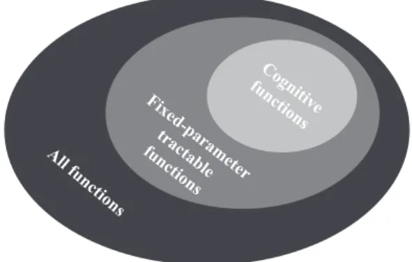
1.2 Conceptual Foundations 19 Cognitive functions Fixed-parameter tractable functions All functions

Figure 1.6 According to theFPT-Cognition thesis, cognitive functions are a subset of all fixed-parameter tractable functions.

is a subset of all fixed-parameter tractable time computable functions (see Figure 1.6). This thesis is called theFPT-Cognition thesis.

With theFPT-Cognition thesis we do not mean to argue thatNP-hardness results are of no significance to cognitive science. On the contrary, the FPT-cognition thesis, like the P-Cognition thesis, recognizes that an NP-hard functionF cannot be practically computed in all its generality. If the system is computing F at all, then it must be computing some “restricted” version of it, denotedF. The crux is, however, what is meant by “restricted.” The P-Cognition thesis states thatFmust be polynomial-time computable, whereas theFPT-cognition thesis states thatFmust have problem parameters that are in practice “small” and thatFmust be fixed-parameter tractable for (a subset of) those parameters.

On the one hand, theFPT-Cognition thesis loses in formality by allowing an undefined notion of “small” parameter in its definition. On the other hand, this allowance is exactly what may bring theFPT-Cognition thesis in closer agreement with cognitive reality. In practice, real-world cognitive inputs seem to have parameters that are of qualitatively different sizes. Ignoring these qualitative differences, and treating the input always as one big “chunk,” would risk making complexity analysis in cognitive science practice vacuous. The FPT-Cognition thesis, then, should not be seen as a simple litmus test for distinguishing feasible from unfeasible computational-level theories. On the contrary, the FPT-Cognition thesis is probably best seen as a stimulans for actively exploring how the inputs of computational-level theories are parametrically constrained in order to guarantee tractability in real-world situations.

(18)

The following chapters will cover proof techniques for assessing whether or not a given function (or problem) F is computable in polynomial time and/or fixed-parameter tractable time. These techniques can then be used to assess whether or not a given computational-level theory meets the tractability constraint, be it formalized as theP- orFPT-Cognition thesis.

1.3

Exercises

In this chapter you learned about the conceptual foundations of the tractability constraint on computational-level theories of cognition. To consolidate your newly gained knowledge you can quiz yourself with the following exercises.

Exercise 1.3.1 We used Subset Choice as a running example. Consider now

a cognitive capacity of special interest to you. Imagine going through the same process of first defining the most general input-output mapping for this capacity and then working toward one that may be tractable. What kinds of input-output mappings would you come up with?

Exercise 1.3.2 Different cognitive scientists have a preference to start the-orizing at one or more of Marr’s levels of explanation. What benefits and drawbacks do you see for starting at the computational level, the algorithmic level, or the implementational level? Try to come up with at least one benefit and drawback for each option.

Exercise 1.3.3 Search for a few cognitive science articles that use the word “intractability.” What is the meaning of the word used in those articles? (Hint: the term “intractability” is often used informally in the cognitive science literature. Regularly, it means “computational intractability,” as we use it throughout this book, but not always. For instance, sometimes it means something like unmanageable, uncontrollable, very difficult, or analytically unsolvable.)

Exercise 1.3.4 Just as the Church-Turing thesis provides a definition of computability independent of the Turing-machine formalization, both the P-Cognition andFPT-Cognition thesis intend to use definitions of tractability that are independent of the Turing-machine formalization. This is afforded by the so-called Invariance thesis, which states that two reasonable com-puting machines can simulate each other with at most polynomial-time overhead. Read the Turing-Machine Objection in Chapter 9, and answer the following question: Why does the Invariance thesis, if true, guarantee that the P-Cognition and FPT-Cognition theses apply to computational-level theories regardless the nature of brain computation?

(19)

1.4 Further Reading 21

1.4