■
Simulation based Bayesian econometric inference:
principles and some recent computational advances
Lennart F. Hoogerheide, Herman K. Van Dijk
and Rutger D. Van Oest
CORE DISCUSSION PAPER 2007/15
Simulation based Bayesian econometric inference: principles and some recent computational advances Lennart F. HOOGERHEIDE1, Herman K. VAN DIJK2
and Rutger D. VAN OEST3
March 2007
Abstract
In this paper we discuss several aspects of simulation based Bayesian econometric inference. We start at an elementary level on basic concepts of Bayesian analysis; evaluating integrals by simulation methods is a crucial ingredient in Bayesian inference. Next, the most popular and well-known simulation techniques are discussed, the Metropolis-Hastings algorithm and Gibbs sampling (being the most popular Markov chain Monte Carlo methods) and importance sampling. After that, we discuss two recently developed sampling methods: adaptive radial based direction sampling [ARDS], which makes use of a transformation to radial coordinates, and neural network sampling, which makes use of a neural network approximation to the posterior distribution of interest. Both methods are especially useful in cases where the posterior distribution is not well-behaved, in the sense of having highly non-elliptical shapes. The simulation techniques are illustrated in several example models, such as a model for the real US GNP and models for binary data of a US recession indicator.
JEL classification: C11, C12, C15, C45, C52
1 CORE, Université catholique de Louvain, Belgium. E-mail: [email protected]
2 Econometric and Tinbergen Institutes, Erasmus University Rotterdam, The Netherlands. E-mail: [email protected]
3 CentER, Faculty of Economics and Business Administration, Tilburg University, The Netherlands. E-mail: [email protected]
This paper presents research results of the Belgian Program on Interuniversity Poles of Attraction initiated by the Belgian State, Prime Minister's Office, Science Policy Programming. The scientific responsibility is assumed by the authors.
1
Introduction
In this paper we discuss several aspects of simulation based Bayesian econometric inference [SBBEI]. In recent decades there has been a huge increase in the use of simulation methods for the Bayesian analysis of econometric models. This ‘Simulation Revolution’ in Bayesian econometric inference is to a large extent due to the advent of computers with ever-increasing computational power; see e.g. the discussion in Geweke (1999), Van Dijk (1999) and Hamilton (2006). This computational power allows researchers to apply elaborate Bayesian simula-tion techniques for estimasimula-tion in which extensive use is made of pseudo-random numbers generated on computers.
The basic principle in this line of research is that in most cases of empirical econometric models one can not directly simulate from the distribution of interest. Thus one applies in such cases an indirect sampling method. Two classes of indirect simulation methods are Importance Sampling and Markov chain Monte Carlo. The theory of Markov chain Monte Carlo [MCMC] methods starts with Metropolis et al. (1953) and Hastings (1970). The Gibbs sampling method, the most well-known MCMC method, is due to Geman and Geman (1984). Importance sampling, due to Hammersley and Handscomb (1964), was introduced in econometrics and statistics by Kloek and Van Dijk (1978), and further developed by Van Dijk and Kloek (1980, 1984) and Geweke (1989).
The Gibbs sampler has, in particular, become a popular tool in econometrics for analyzing a wide variety of problems; see Chib and Greenberg (1995) and Geweke (1999). Judging from numerous articles in recent literature, Gibbs sampling is still gaining more and more momentum. Recent textbooks such as Bauwens, Lubrano and Richard (1999), Koop (2003), Lancaster (2004), and Geweke (2005) discuss how Gibbs sampling is used in a wide range of econometric models, in particular in models with latent variables.
Evaluating integrals is a crucial ingredient in the Bayesian analysis of any model. The reason is that the basic principle, Bayes’ rule, provides (a kernel of) the joint posterior density of all parameters occurring in the model. One is typically interested in the posterior means and standard deviations of some of the parameters; the posterior probability that a parameter lies in a certain interval; and/or the marginal likelihood of the model. For these purposes - and, of course, for prediction and decision analysis - one has to integrate the joint posterior density kernel with respect to all parameters. Therefore, the development of advanced sampling methods, that perform this integration operation efficiently, makes Bayesian inference possible in a wider class of complex models. This allows for more realistic descriptions of processes in many situations, for example in finance and macro-economics, leading to more accurate forecasts and a better quantification of uncertainty.
In order to make this paper self contained we start with a discussion of basic principles of Bayesian inference such as prior and posterior density, Bayes’ rule, Highest Posterior Density [HPD] region, Bayes factor, and posterior odds. Good knowledge of these principles is necessary for understanding the application of simulation methods in Bayesian econometric inference. After the introduction to Bayesian inference we proceed and discuss basic ideas of simulation methods. These methods are applicable to posterior densities that are reasonably well-behaved. Recent work in SBBEI deals with cases where the posterior is not well-behaved. We also discuss some methods that can be used in such a situation. Highly non-elliptical shapes in posterior distributions typically arise when some parameters have a substantial amount of posterior probability near or at the boundary of the parameter region. This feature may occur and is relevant in several econometric models. A practical example is a
2 A PRIMER ON BAYESIAN INFERENCE 2 dynamic economic process that is possibly non-stationary. Other examples are the presence of very weak instruments in an instrumental variable regression model, and models with multiple regimes in which one regime may have neglectable probability.
The contents of this paper is structured as follows. In Section 2 we briefly review the basic principles of Bayesian inference. In Section 3 we first discuss several well-known simulation techniques such as Importance Sampling, the Metropolis-Hastings algorithm and the Gibbs sampler. Next, we discuss two recently developed simulation methods: adaptive radial based direction sampling [ARDS], which makes use of a transformation to radial coordinates, and neural network sampling, which makes use of a neural network approximation to the posterior distribution of interest. The final section provides some concluding remarks.
2
A Primer on Bayesian Inference
2.1 Motivation for Bayesian Inference
The dissatisfaction that many applied economic researchers feel when they consider the ‘significance’ of regression coefficients, using the frequentist/classical approach, is one major motivation to start with Bayesian inference. Consider the following example.
Example: growth of real GNP in the US
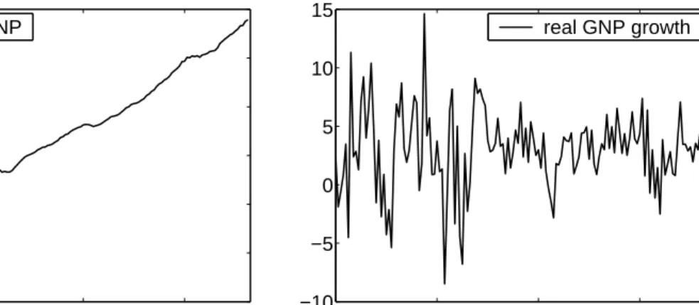
Throughout this paper we use the (annualized) quarterly growth rate of the real Gross Na-tional Product (GNP) in the United States several times for illustrative purposes. The data are shown in Figure 1. Consider the ordinary least squares (OLS) regression forT = 126observations
ytfrom 1975 to the second quarter of 2006 (with t-values in parentheses):
yt = 1.99 + 0.22 yt−1+ 0.13 yt−2 + ˆut (t= 1, . . . , T)
(4.80) (2.57) (1.50)
where uˆt are OLS residuals. Now suppose one fixes the coefficient of yt−2 at zero; then one obtains:
yt = 2.26 + 0.27 yt−1+ ˆvt (t= 1, . . . , T)
(6.03) (3.13)
wherevˆt are the OLS residuals. A naive researcher might conclude that in the second model the influence ofyt−1 onytis “much more significant”. However, according to a proper interpretation of the frequentist/classical approach, this is not a meaningful statement. The reason for this is that in classical inference only the falsification of the null hypothesis is possible. Otherwise stated, it is only relevant whether or not the null hypothesis is rejected.
Another point is that the concept of ‘unbiasedness’ of an estimator is not meaningful in non-experimental sciences: an unbiased estimator takes on average the correct value when the process is repeated (infinitely) many times. However, in non-experimental sciences this idea
19700 1980 1990 2000 20 40 60 80 100 120 real GNP 1970 1980 1990 2000 −10 −5 0 5 10 15 real GNP growth
Figure 1: U.S. real Gross National Product - quantity index, 2000=100 (left), and corre-sponding (annualized) growth rates in percents (right). The data are seasonally adjusted. Source: U.S. Department of Commerce, Bureau of Economic Analysis.
of repeating the process is not realistic. In non-experimental sciences, a researcher cannot repeat the process he/she studies, and he/she has to deal with only one given data set.
A proper way to consider the sensitivity of estimates and to use probability statements that indicate a ‘degree of confidence’ is given by the framework of Bayesian inference. So, apart from dissatisfaction with existing practice of the frequentist/classical approach, there also exists a constructive motive to apply Bayesian inference. That is, a second major motivation to start with Bayesian inference is that the Bayesian framework provides a natural learning rule, that allows for optimal learning and (hence) optimal decision making under uncertainty.
In this section the basic principle of Bayesian inference, Bayes’ theorem, will first be discussed. After that, some concepts that play an important role within the Bayesian frame-work will be described, and a comparison will be made between Bayesian inference and the frequentist/classical approach.
2.2 Bayes’ theorem as a learning device
Econometric models may be described by the joint probability distribution ofy={y1, . . . , yN},
the set ofN available observations on the endogenous variableyi, whereyi may be a vector
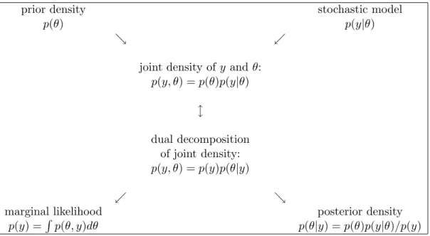
itself, that is known up to a parameter vectorθ. Bayesian inference proceeds from the likeli-hood functionL(θ) =p(y|θ), which is either the density of the data given the parameters in case of a continuous distribution or the probability function in case of a discrete distribution, and a prior density p(θ) reflecting prior beliefs on the parameters before the data set has been observed. So, in the Bayesian approach the parameters θ are considered as random variables of which the prior densityp(θ) is updated by the information contained in the data, incorporated in the likelihood functionL(θ) =p(y|θ), to obtain the posterior density of the parametersp(θ|y). This process is formalized by Bayes’ theorem:
p(θ|y) = p(θ)p(y|θ)
p(y) . (1)
Note that this is merely a result of rewriting the identityp(y)p(θ|y) = p(θ)p(y|θ), the two ways of decomposing the joint densityp(y, θ) into a marginal and a conditional density; see
2 A PRIMER ON BAYESIAN INFERENCE 4
prior density stochastic model
p(θ) p(y|θ)
& .
joint density ofy and θ: p(y, θ) =p(θ)p(y|θ) l dual decomposition of joint density: p(y, θ) =p(y)p(θ|y) . &
marginal likelihood posterior density
p(y) =R p(θ, y)dθ p(θ|y) =p(θ)p(y|θ)/p(y) Figure 2: Bayes’ theorem as a learning device
Figure 2 for a graphical interpretation of Bayes’ theorem. Notice that one starts with a certain stochastic model with likelihood function p(y|θ) and a prior density function p(θ). Multiplying these two functions yields the joint density ofθandy. Substituting our observed data set y into this joint density yields a function of only θ: a kernel (=proportionality function) of the posterior density ofθ. This kernel merely has to be divided by a constant, the marginal likelihood p(y) = R p(θ, y)dθ = Rp(y|θ)p(θ)dθ, in order to make it a proper (posterior) density function. The marginal likelihood is the marginal density of the data y, after the parameters θ of the model have been integrated out with respect to their prior distribution. The marginal likelihood can be used for model selection, see subsection 2.3.
Formula (1) can be rewritten as:
p(θ|y)∝p(θ)p(y|θ), (2) where the symbol∝means “is proportional to”, i.e. the left-hand side is equal to the right-hand side times a scaling constant (1/p(y) = 1/R p(θ)p(y|θ)dθ) that does not depend on the parametersθ; just like the integrating constant 1/√2π in the standard normal density.
The basic idea behind the Bayesian approach is that the prior densityp(θ) and the pos-terior densityp(y|θ) aresubjective evaluations of possible states of nature and/or outcomes of some process (or action). A famous quote of De Finetti (1974) is: “probabilities do not exist”, that is, probabilities are not physical quantities that one can measure in practice, but they are states of the mind.
Bayes’ rule can be interpreted as follows. One starts with the prior density p(θ); this contains intuitive, theoretical or other ideas on θ, that may stem from earlier or parallel studies. Then one learns from data through the likelihood function p(y|θ). This yields the posterior p(θ|y). Briefly stated, Bayes’ paradigm is a learning principle, which can be depicted as follows:
posterior density ∝ prior density × likelihood beliefs after ⇐ beliefs before & influence having observed data observing data of the data
Note that we can apply Bayes’ rule sequentially: when new data will become available, we can treat the posterior density that is based on the current data set as the prior density.
The key problems in Bayesian inference are the determination of the probability laws in the posterior kernel, i.e. what families of posterior densities are defined, and the computation of the marginal likelihood.
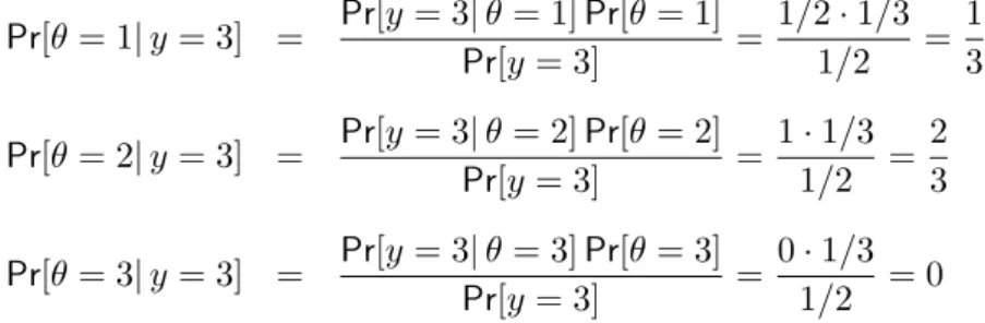
Example: illustration of Bayes’ rule in TV show game (Monty Hall problem)
We illustrate the application of Bayes’ rule in a simple example of a game that was played in the American TV show ‘Let’s make a deal’. It is known as the Monty Hall problem, after the show’s host. In this TV show game, one could win a car by choosing among three doors the door behind which a car was parked. The candidate was faced with three closed doors: behind one door there was a car, behind the other two doors there was nothing.1 The procedure of the game
was as follows. First, the candidate chose one door, say door 1. Second, the TV show host - who knew behind which door the car could be found - opened one of the other two doorswith no car behind it. So, if the car was behind door 2, the show’s host opened door 3, and vice versa. If the car was behind door 1, the host would open either door 2 or 3 with probability 1/2. Suppose that after the candidate had chosen door 1, the presenter opened door 3. Finally, the candidate got the chance to switch his/her choice from his/her initial choice (door 1) to the other closed door (door 2). Throughout the episodes of the TV show there were many candidates who chose to stick with their initially chosen door. The question is now whether this was a wise decision; or stated otherwise, was this rationally an optimal decision? To answer this question, we will make use of Bayes’ rule.
In order to be able to apply Bayes’ rule in this example, we must formulate the TV show game as a model. In this model there is one parameterθ reflecting the door with the car behind it, θ∈ {1,2,3}. The data y are given by the door that the host opens after the candidate has chosen door 1,y∈ {2,3}. We assume that there is no prior preference for one of the three doors: Pr[θ=i] = 1/3 fori= 1,2,3. In the case in which the host opens the third door, the likelihood is given by: Pr[y= 3|θ= 1] = 1/2, Pr[y = 3|θ= 2] = 1, Pr[y= 3|θ= 3] = 0.
From the prior and the likelihood we can now obtain the posterior probability distribution of
θusing Bayes’ rule. First we obtain the marginal likelihood:2
Pr[y= 3] = 3 X j=1 Pr[y= 3|θ=j]Pr[θ=j] = 1 2· 1 3 + 1· 1 3 + 0· 1 3 = 1 6 + 1 3 = 1 2
1The Monty Hall problem is also described as the situation with a car behind one door and a goat behind
the other two doors. Obviously, this does not intrinsically change the situation: the point is that behind one door there is something that is worth considerably more money than what is behind the other two doors.
2Note that we have a summation over the domain ofθhere (instead of an integral), because this is a (quite
2 A PRIMER ON BAYESIAN INFERENCE 6
Now we obtain the posterior probabilities:
Pr[θ= 1|y= 3] = Pr[y= 3|θ= 1]Pr[θ= 1] Pr[y= 3] = 1/2·1/3 1/2 = 1 3 Pr[θ= 2|y= 3] = Pr[y= 3|θ= 2]Pr[θ= 2] Pr[y= 3] = 1·1/3 1/2 = 2 3 Pr[θ= 3|y= 3] = Pr[y= 3|θ= 3]Pr[θ= 3] Pr[y= 3] = 0·1/3 1/2 = 0
We conclude that it would actually be the best rational decision to switch to door 2, having a (posterior) probability of 2/3, whereas door 1 merely has a (posterior) probability of 1/3. The problem is also called the Monty Hallparadox, as the solution may be counterintuitive: it may appear as if theseemingly equivalent doors 1 and 2 should have equal probability of 1/2. However, the following reasoning explains intuitively why the probability that the car is behind door 1 is merely 1/3, after door 3 has been opened. At the beginning the probability that the car is behind door 1 was 1/3, and the fact that door 3 is opened does not change this: it is already known in advance that the host will open one of theother doorswith no car behind it. In other words, the data do not affect the probability that the car is behind door 1. So after door 3 has been opened, door 1 still has 1/3 probability, while door 2 now has the 2/3 probability that doors 2 and 3 together had before door 3 had been opened.
It is interesting to see which decision would result from the maximum likelihood approach in this case. Here the ML approach would yield the same decision: θˆM L = 2. The likelihood Pr[y = 3|θ]is highest for θ = 2: Pr[y = 3|θ = 2] = 1. However, it should be noted that the ML approach does not immediately indicate what the probability is that the car is behind door 2; it does not immediately reveal the uncertainty about the decision. Moreover, if one would have the prior information that in 3 out of 5 TV shows the car is behind door 1, and in 1 out of 5 shows behind door 2 or door 3, then the Bayesian approach would yield a different choice than the ML approach. Then θˆM L would still be θˆM L = 2, whereas the posterior probabilities would then be Pr[θ= 1|y= 3] = 3/5versus Pr[θ= 2|y= 3] = 2/5. This illustrates how Bayes’ rule provides us with a natural method to include prior information that is relevant for optimal decision making, and to assess the uncertainty about this decision.
Example: growth of real GNP in the US (continued)
We now illustrate Bayes’ theorem in a simple model for the quarterly data on U.S. real GNP. Figure 1 displays real GNP and the corresponding growth rate in percents. Here we consider the naive model
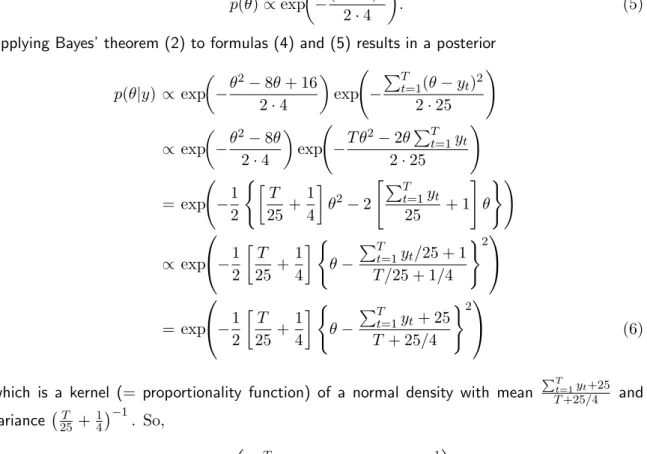
yt=θ+εt, εt∼ N(0,25) i.i.d., t= 1, . . . , T, (3)
whereytis the (annualized) growth rate in periodtandθis the average growth rate. So, growth rates are assumed to obey a normal distribution with known standard deviation 5. Clearly, the likelihood function is given by
p(y|θ)∝exp à − PT t=1(yt−θ)2 2·25 ! , (4)
where we have omitted the scaling constant of the normal density, as it is irrelevant in the analysis. Next, a prior density has to be specified forθ. Suppose that it is a priori expected that average real GNP growth is approximately 4 (percent), and that one believes that there is a 95% probability that average real GNP growth lies between 0 and 8 (percent). Such prior beliefs can be captured by a normal distribution with mean 4 and standard deviation 2 (percent), so that the prior density is given by
p(θ)∝exp µ −(θ−4) 2 2·4 ¶ . (5)
Applying Bayes’ theorem (2) to formulas (4) and (5) results in a posterior
p(θ|y) ∝ exp µ −θ2−8θ+ 16 2·4 ¶ exp à − PT t=1(θ−yt)2 2·25 ! ∝ exp µ −θ2−8θ 2·4 ¶ exp à −T θ2−2θ PT t=1yt 2·25 ! = exp à −1 2 (· T 25 + 1 4 ¸ θ2−2 " PT t=1yt 25 + 1 # θ )! ∝ exp −1 2 · T 25 + 1 4 ¸ ( θ− PT t=1yt/25 + 1 T /25 + 1/4 )2 = exp −1 2 · T 25 + 1 4 ¸ ( θ− PT t=1yt+ 25 T+ 25/4 )2 (6)
which is a kernel (= proportionality function) of a normal density with mean PTt=1yt+25
T+25/4 and variance¡25T +14¢−1. So, θ|y ∼ N Ã PT t=1yt+ 25 T + 25/4 , µ T 25+ 1 4 ¶−1! . (7)
Note that for T → ∞ the posterior mean of θ approaches the sample mean PTt=1yt/T and the posterior variance goes to 0, whereas filling in T = 0 (and PTt=1yt = 0) yields the prior distribution.
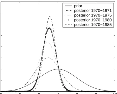
Figure 3 provides a graphical illustration of Bayesian learning. It shows how the distribution of the real GNP growth parameterθ changes when more observations become available. In the graph, the posterior distributions are obtained from (7), where the considered observations run from 1970 to 1971, 1975, 1980 and 1985, respectively. For instance, the first posterior density includes the years 1970 and 1971, that is, 8 quarterly observations. All the posterior distributions are located to the left of the prior, suggesting that the prior belief of 4 percent growth overes-timates the actual growth rate. It is further seen that parameter uncertainty is reduced when more observations are used.
2 A PRIMER ON BAYESIAN INFERENCE 8 −20 0 2 4 6 8 10 0.1 0.2 0.3 0.4 0.5 0.6 0.7 0.8 prior posterior 1970−1971 posterior 1970−1975 posterior 1970−1980 posterior 1970−1985
Figure 3: Illustration of Bayesian learning: average U.S. real GNP growth.
Conjugate priors
The example above demonstrates that a normal prior applied to a normal data generating process results in a normal posterior. This phenomenon that the posterior density has the same form as the prior density is called “conjugacy”. Conjugate priors are useful, as they greatly simplify Bayesian analysis. There exist several forms of conjugacy. Without the intention to be exhaustive, we mention that a Beta prior results in a Beta posterior for a binomial data process, and that a gamma prior results in a gamma posterior for a Poisson data process. Although using conjugacy facilitates Bayesian analysis, a possible critical re-mark is that conjugate priors are often more driven by convenience than by realism.
General case of the normal model with known variance
The example above can be generalized. Suppose that the data y = (y1, . . . , yT) are
gen-erated from a normal distribution N(θ, σ2) where the variance σ2 is known, and the prior distribution for the parameterθisN(θ0, σ02). So, we consider the same model as before, but now we do not fill in specific values for the process varianceσ2 and the prior parameters θ
0 andσ2
0. In a similar fashion as before, it can be shown that for this more general case θ|y∼ N Ã θ0σ2+σ20 PT t=1yt σ2+T σ2 0 , µ 1 σ2 0 + T σ2 ¶−1! . (8)
Interestingly, both the posterior expectation and the (inverse of the) posterior variance in (8) can be decomposed into a prior component and a sample component. By defining the
sample mean ˆθ= T1 PTt=1yt and its varianceσ2θˆ= σ 2 T , (8) can be written as θ|y∼ N Ã σ0−2 σ−02+σ−ˆ2 θ θ0+ σ−ˆ2 θ σ0−2+σ−ˆ2 θ ˆ θ, ³ σ0−2+σ−ˆ2 θ ´−1! . (9)
In order to interpret (9), we note that the inverted variancesσ0−2andσ−ˆ2
θ essentially measure
the informativeness of prior beliefs and available data, respectively. For instance, ifσ−02 is much smaller thanσ−ˆ2
θ , then the prior density is flat relative to the likelihood function, so
that the shape of the posterior density is mainly determined by the data. It is seen from (9) that the posterior expectation ofθ is a weighted average of the prior expectationθ0 and the sample mean ˆθ; the weights reflect the amount of prior information relative to the available sample information.
A practical problem, which we have ignored in the analysis so far, is that prior beliefs are often difficult to specify and extremely subjective. So, it might happen that researchers strongly disagree on which prior density is appropriate for the inference problem. As prior beliefs directly affect the posterior results, different researchers may arrive at different con-clusions. In order to reach some form of consensus, non-informative priors are therefore frequently considered. Such priors are constructed in such a way that they contain little information relative to the information coming from the data. In the (generalized) example above, a “non-informative” prior can be obtained by making the prior distributionN(θ0, σ2
0) diffuse, that is, by letting the prior varianceσ2
0 go to infinity. This essentially amounts to choosing a uniform priorp(θ)∝1, reflecting no a priori preference for specificθvalues. This implies that the posterior becomes proportional to the likelihood function. It immediately follows from (9) that an infinitely large prior variance results in
θ|y∼ N(ˆθ, σ2ˆ
θ), (10)
which shows a nice symmetry with classical maximum likelihood [ML], as the ML estimator ˆ
θ is N(θ, σ2θˆ) distributed. Note that to do classical inference some “true” value has to be assumed for the unknown parameterθ, as otherwise the distributionN(θ, σ2
ˆ
θ) would contain
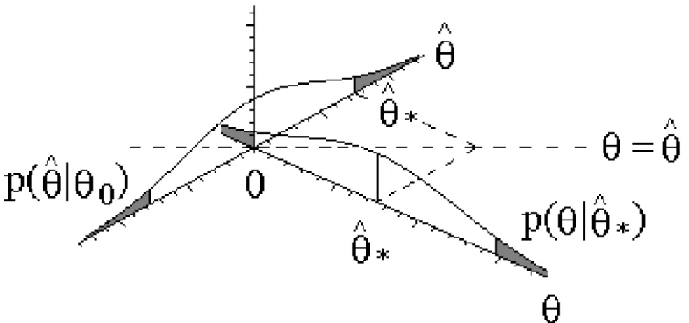
unknown elements. Classical analysis is conditioned on postulated “true” parameter val-ues, whereas Bayesian analysis is conditioned on the data. This is an important difference between the two approaches. Figure 4 illustrates the difference between the Bayesian and frequentist approach in our simple linear model with known variance. A Bayesian may inves-tigate whether zero is a likely value forθgiven the data (summarized in ˆθ∗, the sample mean
of the observed datayt (t= 1, . . . , T)), by inspecting the posterior density p(θ|θˆ∗) at θ= 0.
On the other hand, a frequentist may analyze whether the data – again summarized in the sample mean ˆθ∗ – are likely under the hypothesis that the true value isθ
0 = 0, by comparing ˆ
θ∗ with the density p(ˆθ|θ
0) of an (infinitely large) set of sample means ˆθ of (hypothetical) data sets that are generated from the model underθ0= 0.
2 A PRIMER ON BAYESIAN INFERENCE 10
Figure 4: Illustration of symmetry of Bayesian inference and frequentist approach in linear regression model and difference between these approaches
2.3 Model evaluation and model selection
In this section, we discuss two Bayesian testing approaches for model selection. The first is based on the highest posterior density [HPD] region, which is the Bayesian counterpart of the classical confidence interval. The second is posterior odds analysis, comparing the probabilities of multiple considered models given the available data. An important difference between the two approaches is that tests using the HPD region are based on finding evidence against the null model, whereas posterior odds analysis considers the evidence in favor of each of the models under scrutiny. So, the HPD approach treats models in an asymmetrical way, just like frequentist/classical testing procedures. The posterior odds approach treats models symmetrically.
2.3.1 The HPD region
The highest posterior density [HPD] region is defined such that any parameter point inside that region has a higher posterior density than any parameter point outside. Consequently, the usually considered 95% HPD region is the smallest region containing 95% of the posterior probability mass. We note that an HPD region does not necessarily consist of a single interval. For example, it might consist of two intervals if the posterior density is bimodal.
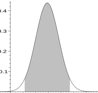
Figure 5 shows the 95% HPD region for the average real GNP growth rate θ in the normal model with known variance. The standard normal distribution has 2.5% probability mass both to the right of 1.96 and to the left of−1.96, so that the 95% HPD region forθis (2.92−1.96·0.91, 2.92 + 1.96·0.91) = (1.14,4.70). It is seen from Figure 5 that a real GNP model imposing zero average growth is rejected, asθ= 0 is located outside the HPD region. Although the Bayesian HPD region has similarities with the classical confidence interval, the interpretations are very different. In the classical framework, the confidence interval (constructed from the data) is considered random and the postulated parameter value is given, so that one effectively tests whether the data are plausible for the assumed parameter value. On the other hand, a Bayesian considers the HPD region as given and the parameter outcome as random, so that it is effectively tested whether the parameter outcome is plausible given the available data.
0.1 0.2 0.3 0.4 –1 1 2 3 4 5 6 7 θ
Figure 5: 95% HPD region for the average real GNP growth rate θ based on 24 quarterly observations from 1970 to 1975
2.3.2 Posterior odds analysis
An HPD region based test considers the amount of evidence against the null model, but it does not say anything about the amount of evidence in favor of the alternative model relative to the null model. So, the null model and the alternative model are treated asymmetrically. A testing approach in which models are directly compared is posterior odds analysis. Its formalization for two possiblynon-nested competing modelsM1 andM2is as follows. Given the available datay, the model probabilities areP r(M1|y) andP r(M2|y), whereP r(M1|y)+ P r(M2|y) = 1. Using Bayes’ theorem, we can write these model probabilities as
P r(M1|y) = p(Mp(1y), y) = P r(M P r(M1)p(y|M1) 1)p(y|M1) +P r(M2)p(y|M2), (11) P r(M2|y) = p(M2, y) p(y) = P r(M2)p(y|M2) P r(M1)p(y|M1) +P r(M2)p(y|M2) . (12)
Theposterior odds ratio in favor of model 1, that is, the ratio of (11) and (12), is now defined by K1,2= P r(M1|y) P r(M2|y) = P r(M1) P r(M2) p(y|M1) p(y|M2) . (13)
Model 1 is preferred if K1,2 is larger than 1, and model 2 is preferred in the opposite case. The relationship (13) states that the posterior odds ratio K1,2 equals the prior odds ratio
P r(M1)
P r(M2), reflecting prior model beliefs, times the so-called Bayes factor B1,2= pp((yy||MM1)
2 A PRIMER ON BAYESIAN INFERENCE 12 accounting for the observed datay. We note that the posterior odds ratio equals the Bayes factor if the two models are a priori assumed to be equally likely, that is, if P r(M1) = P r(M2) = 0.5. The subsequent discussion on Bayes factors is quite brief, but a more extensive treatment can be found in Kass and Raftery (1995).
The Bayes factorB1,2 is the ratio of the marginal likelihoods p(y|M1) = Z p(y|θ1, M1)p(θ1|M1)dθ1, (15) p(y|M2) = Z p(y|θ2, M2)p(θ2|M2)dθ2, (16) where θ1 and θ2 are the parameter vectors in the two models, and where the prior densities p(θ1|M1) and p(θ2|M2) and the likelihood functions p(y|θ1, M1) and p(y|θ2, M2) contain all scaling constants. It is interesting to note that the Bayes factor is closely related to the likelihood ratio. However, the latter maximizes over the model parameters, whereas the former integrates them out. Furthermore, if both the models M1 and M2 do not contain free parameters, then the Bayes factor is just the ratio of two likelihoods evaluated at fixed parameter values.
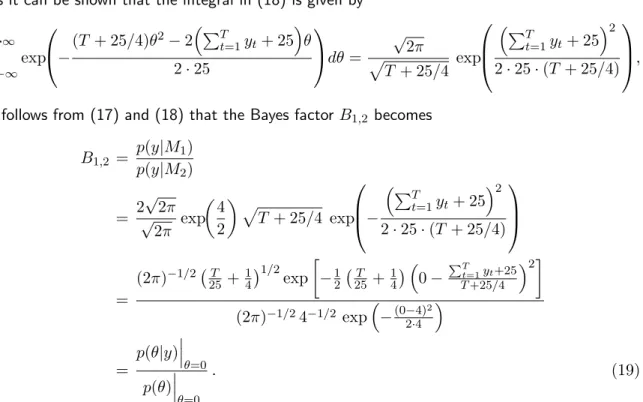
Example: growth of real GNP in the US (continued)
As an illustration, we consider the normal real GNP growth model with standard deviation 5. As before, the average growth parameter θ has a normal prior density with mean 4 and standard deviation 2. We use Bayes factors to compare the zero growth modelM1, imposing that θ= 0,
with the unrestricted modelM2. As modelM1 does not contain free parameters, the marginal
likelihood for this model is just the likelihood function evaluated atθ= 0, that is,
p(y|M1) =p(y|θ= 0) = (2π·25)−T /2exp à − PT t=1yt2 2·25 ! . (17)
Furthermore, the marginal likelihood for modelM2 is p(y|M2) = Z ∞ −∞ p(y|θ, M2)p(θ|M2)dθ = Z ∞ −∞ (2π·25)−T /2exp à − PT t=1(yt−θ)2 2·25 ! (2π·4)−1/2exp µ −(θ−4) 2 2·4 ¶ dθ = (2π·25)−T /2exp à − PT t=1yt2 2·25 ! 1 2√2π exp µ −4 2 ¶ × × Z ∞ −∞ exp −(T + 25/4)θ 2−2³PT t=1yt+ 25 ´ θ 2·25 dθ. (18)
As it can be shown that the integral in (18) is given by3 Z ∞ −∞ exp −(T + 25/4)θ 2−2³PT t=1yt+ 25 ´ θ 2·25 dθ= √ 2π p T + 25/4 exp ³PT t=1yt+ 25 ´2 2·25·(T+ 25/4) ,
it follows from (17) and (18) that the Bayes factorB1,2 becomes B1,2 = pp((yy||MM1) 2) = 2 √ 2π √ 2π exp µ 4 2 ¶ p T+ 25/4 exp − ³PT t=1yt+ 25 ´2 2·25·(T + 25/4) = (2π)−1/2¡T 25 +14 ¢1/2 exp · −12¡25T +14¢ ³0−PTt=1yt+25 T+25/4 ´2¸ (2π)−1/24−1/2 exp³−(0−4)2 2·4 ´ = p(θ|y) ¯ ¯ ¯ θ=0 p(θ) ¯ ¯ ¯ θ=0 . (19)
the ratio of the posterior density and the prior density, both evaluated at the restricted parameter valueθ= 0.
Savage-Dickey density ratio
The remarkable result in the example above, that the Bayes factor is the ratio of the pos-terior density and the prior density, evaluated at the restricted parameter value, is not a coincidence. It is a special case of the Savage-Dickey density ratio (Dickey 1971). We note that the result above can also be derived immediately from Bayes’ theorem (1) by evaluating it forθ= 0 and rearranging it as
p(θ|y) ¯ ¯ ¯ θ=0 p(θ) ¯ ¯ ¯ θ=0 = p(y|θ= 0) p(y) = p(y|M1) p(y|M2). (20)
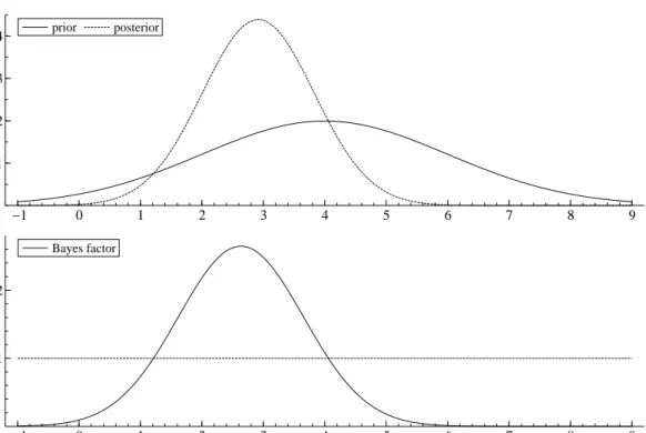
Figure 6 provides a graphical illustration of the result. It shows that forθ= 0 the unrestricted modelM2 is preferred over the restricted modelM1, as the Bayes factorB1,2 is smaller than 1. Note that in the HPD approach the restricted model is also rejected (Figure 5). However, it is certainly possible that the HPD approach and the Bayes factor give different ‘signals’. For example, the value θ = 4.5 is not rejected by the HPD approach, whereas the Bayes factor favors the unrestricted model (Figure 6).
We note that the Savage-Dickey density ratio (20) implies that the restricted modelM1 would always be favored if the prior for the restricted parameters θ is improper (= not
2 A PRIMER ON BAYESIAN INFERENCE 14 −1 0 1 2 3 4 5 6 7 8 9 0.1 0.2 0.3 0.4 prior posterior −1 0 1 2 3 4 5 6 7 8 9 1 2 Bayes factor
Figure 6: Prior and posterior densities for the average (annualized) real GNP growth rate, where the posterior involves 24 quarterly observations from 1970 to 1975 (above), and the Bayes factor to test that the average growth rate equals the value on the horizontal axis (below).
integrating to a constant, “infinitely diffuse”), as the denominator in the Bayes factorB1,2 would tend to zero. This phenomenon is the Bartlett paradox (Lindley 1957, Bartlett 1957). It demonstrates that, at least for the parameters being tested, improper priors should be avoided in posterior odds analysis.
Example: illustration of Bayes’ rule, HPD region and posterior odds in World Series Consider the following illustrative, simple model for the World Series 2004 between the Boston Red Sox and the St. Louis Cardinals. In this model we have datay ={y1, . . . , yn} with
yt=
½
1 Boston Red Sox win match t
0 St. Louis Cardinals win match t , t= 1, . . . , T.
that are assumed independently Bernoulli(θ) distributed, i.e. the model contains only one pa-rameter θ, the probability that the Boston Red Sox beat the St. Louis Cardinals in match t
(t= 1, . . . , T). The probability distribution of yt (t= 1, . . . , T) is: Pr[yt|θ] =θyt(1−θ)1−yt
leading to the likelihood: Pr[y|θ] = T Y t=1 Pr[yt|θ] =θT1(1−θ)T2
with T1 and T2 the numbers of matches that have been won by the Boston Red Sox and the
St. Louis cardinals, respectively. Suppose we have no a priori preference for the parameterθ, so we specify a uniform prior: p(θ) = 1 forθ∈[0,1],p(θ) = 0 else.
In the year 2004 the World Series consisted of only 4 matches that were all won by the Boston Red Sox, soyt = 1for t= 1,2,3,4. Hence, after T of these matches the likelihood is given by Pr[yi|θ] =θT, and the posterior density of θis given by
p(θ|y)∝Pr[yt|θ]p(θ) =
½
θT 0≤θ≤1
0 else
forT = 1,2,3,4. The scaling constant RPr[yt|θ]p(θ)dθ is
Z Pr[yt|θ]p(θ)dθ= Z 1 0 θTdθ= 1 T+ 1 so we have p(θ|y) = R Pr[yt|θ]p(θ) Pr[yt|θ]p(θ)dθ = ½ (T+ 1)θT 0≤θ≤1 0 else .
Figure 7 shows the graphs of the prior and posterior density ofθafterT = 1,2,3,4matches. Note that after each match - won by the Boston Red Sox - more density mass is located on the right side of θ = 0.5. The posterior cumulative distribution function [CDF] of θ after T = 1,2,3,4
matches is given by P r[θ ≤ θ˜] = ˜θT+1. So, the 95% HPD region is given by [0.051/(T+1),1].
The 95% HPD region is [0.22,1], [0.37,1], [0.47,1], [0.55,1] after T = 1,2,3,4 observations, respectively.
We now consider a posterior odds analysis for the following two modelsM1 andM2: model M1 in whichθ≤1/2and modelM2in which θ >1/2. Models 1 and 2 can be interpreted as the
hypotheses that “the St. Louis Cardinals are at least as good as the Boston Red Sox” and “the Boston Red Sox are better than the St. Louis Cardinals”, respectively. The prior distributions for
θunder models 1 and 2 are assumed to be uniform on [0,1/2]and(1/2,1], respectively. Notice that the modelsM1 andM2 are non-nested. In the case in which the Boston Red Sox have won
all matches, the marginals likelihoods are given by:
p(y|M1) = Z p(y|θ, M1)p(θ|M1)dθ= Z 1/2 0 θT2dθ= 2 T+ 1 µ 1 2 ¶T+1 , p(y|M2) = Z p(y|θ, M2)p(θ|M2)dθ= Z 1 1/2 θT2dθ = 2 T+ 1 " 1− µ 1 2 ¶T+1# .
So, if we assume equal prior probabilitiesP r[M1] = P r[M2] = 0.5, then the Bayes factor and
posterior odds ratioK1,2 are given by:
K1,2 ≡ P rP r[[MM1|y] 2|y]
= (1/2)T+1 1−(1/2)T+1.
The posterior probabilities of models M1 and M2 are given by P r[M1|y] = (1/2)T+1 and P r[M2|y] = 1−(1/2)T+1. So, the probability that “the St. Louis Cardinals are at least as
2 A PRIMER ON BAYESIAN INFERENCE 16
0
0.2
0.4
0.6
0.8
1
0
1
2
3
4
5
θ
p(
θ
)
p(
θ
|y) T = 1
p(
θ
|y) T = 2
p(
θ
|y) T = 3
p(
θ
|y) T = 4
Figure 7: Prior density and posterior density of parameter θ (probability that Boston Red Sox win a match) afterT = 1,2,3,4matches (that are won by the Boston Red Sox) in World Series of the year 2004.
good as the Boston Red Sox” given T (T = 1,2,3,4) observed matches (won by the Boston Red Sox) isP r[M1|y] = (1/2)T+1, which equals 0.25, 0.125, 0.06 and 0.03 forT = 1,2,3,4.
We now compare these conclusions of Bayesian methods with the frequentist/classical ap-proach. In the frequentist/classical framework, a test of null hypothesis H0 : θ ≤ 0.5 versus
alternative hypothesisH1 :θ >0.5(using the number of matches won by the Boston Red Sox as
a test statistic) has p-value(1/2)T afterT (T = 1,2,3,4) matches. After four matches we have a p-value of 0.06, so that at 5% size we can not even reject the null. Note that the posterior odds analysis already leads to a ‘preference’ of the Boston Red Sox over the St. Louis Cardinals after one match, whereas four matches are ‘enough’ to make the HPD region based approach lead to a rejection ofθ= 0.5.
2.4 Comparison of Bayesian inference and frequentist approach
In the previous subsections we have considered the principles of Bayesian inference. In order to gain more insight into the key elements of Bayesian inference, we now conclude this section with a brief comparison between Bayesian inference and the frequentist/classical approach. Table 1 provides an overview of four points at which these two approaches differ; for four
Table 1: Comparison of frequentist (or classical) approach and Bayesian approach in a sta-tistical/econometric model with parameter vectorθ and data y
Frequentist approach Bayesian approach
The parametersθare fixed unknown con-stants. There is some unknown true value θ=θ0.
The parametersθare stochastic variables. One defines a prior distribution on the pa-rameter space. All values in a certain re-gion are possible with a certain probability density.
The data y are used to estimate and check the validity of the postulated null model, by comparing data with an (in-finitely large, hypothetical) data set from the null model.
The datay are used as evidence to update the state of the mind: data transform the prior into the posterior distribution by the likelihood.
Frequency concept of probability : a prob-ability is the fraction of occurrences when a process is repeated infinitely often. It should be noted that, although the fre-quentist approach is often used in non-experimental sciences, repeating the pro-cess is only possible in experimental situ-ations.
Subjective concept of probability : a prob-ability is a degree of belief that an event occurs. This degree of belief is revised when new information becomes available.
One can use the maximum likelihood esti-mator ˆθ ofθ as an estimator ofθ.
One uses Bayes’ theorem to obtain the posterior distribution of θ. One can use the posterior mean or mode as an estima-tor ofθ.
elements of Bayesian inference the frequentist counterpart is given. Note that at some points the frequentist approach and Bayesian inference are each other’s opposite. In the frequentist approach, the data are random and the parameters are fixed. Many realizations ˆθare possible under the assumptionθ =θ0. Testing the hypothesis θ= θ0 amounts to checking whether the observed realization ˆθ∗ isplausible underθ=θ0 using the sampling density of ˆθ. So, one checks whether the observed data realization isplausible, while (infinitely) many realizations are possible. On the other hand, in the Bayesian approach the parameters are random, whereas the data are given. Testing the hypothesisθ=θ0 amounts to checking whether the value ofθ0 isplausible given the data. So, (infinitely) many values ofθ arepossible, but one checks whetherθ=θ0 isplausible under theone data realization.
3 SIMULATION METHODS 18
3
Simulation Methods
3.1 Motivation for Using Simulation Techniques
The importance of integration in Bayesian inference can already be seen from the results in the previous section:
• In order to obtain the exact posterior density from Bayes’ theorem one needs to evaluate the integral p(y) =Rp(y|θ)p(θ)dθ in the denominator of (1).
• In order to evaluate the posterior mean of (the elements of)θ, one requires additional integration. For this purpose, two integrals have to be evaluated:
E[θ|y] = Z θp(θ|y)dθ= Z θR p(y|θ)p(θ) p(y|θ)p(θ)dθdθ= R θp(y|θ)p(θ)dθ R p(y|θ)p(θ)dθ .
• In order to evaluate the posterior odds ratio in favor of model 1 versus model 2, one needs to evaluate two marginal likelihoods, and hence two integrals.
In linear and binomial models (for certain prior specifications) these integrals can be com-puted analytically. However, for more complicated models it is usually impossible to find analytical solutions. In general, we need numerical integration methods for Bayesian infer-ence. Basically there are two numerical integration methods: deterministic integration and Monte Carlo integration. Deterministic integration consists of evaluating the integrand at a set of many fixed points, and approximating the integral by a weighted average of the func-tion evaluafunc-tions. Monte Carlo integrafunc-tion is based on the idea thatE[g(θ)|y], the mean of a certain functiong(θ) under the posterior, can be approximated by its ‘sample counterpart’, the sample mean 1
n
Pn
i=1g(θi), whereθ1, . . . , θn are drawn from the posterior distribution. At a first glance, deterministic integration may always seem a better idea than Monte Carlo integration, as no extra uncertainty (caused by the required random variables) is added to the procedure. However, in deterministic integration the number of required function evaluations increases exponentially with the dimension of the integration problem, which is in our case the dimensionkof the vectorθ. Therefore, deterministic integration approaches like quadrature methods become unworkable if k exceeds, say, three. So, in many cases one has to make use of Monte Carlo integration. However, only for a very limited set of models and prior densities it is possible to directly draw random variables from the posterior distribution. In general, direct sampling from the posterior distribution of interest is not possible. Then one may use indirect sampling algorithms such as importance sampling or Markov chain Monte Carlo [MCMC] methods such as the Metropolis-Hastings algorithm. In the following subsections direct sampling methods, importance sampling and MCMC methods will be discussed.
3.2 Direct sampling methods
Only in the ideal case, Monte Carlo integration reduces to estimating the posterior expecta-tionE[g(θ)|y] by the sample meangDS= 1
n
Pn
i=1g(θi), whereθ1, . . . , θnare directly sampled
from the posterior. However, even when the posterior distribution is non-standard, direct sampling methods are useful, as they can serve as building blocks for more involved algo-rithms. For example, any sampling algorithm is based on collecting draws from the uniform U(0,1) distribution, so that suitable methods to generate these “random numbers” are of utmost importance.
3.2.1 Uniform sampling
The most commonly used method to sample from the uniform distribution is the linear congruential random number generator [LCRNG], initially introduced by Lehmer (1951). This generator creates a sequence of “random numbers”u1, . . . , un using the recursion
ui = (a ui−1+b) modM, i= 1, . . . n, (21) where modM gives the remainder after division byM. The multiplieraand the modulusM are strictly positive integers, while the incrementbis also allowed to be zero. The initial value u0 of the sequence is called the seed. In order to mapu1,. . .,un to the unit interval, these
values are divided byM. We note that the recursion (21) is completely deterministic, so that the generated “random numbers” are actually not random at all. For properly chosena,band M, it only seemsas if they are random. In practice, multiplicative LCRNGs are frequently considered. These arise from (21) by setting b = 0, so that the increment is turned off. Two very popular multiplicative LCRNGs are the Lewis-Goodman-Miller generator (Lewis et al. 1969), obtained by settinga= 16807 andM = 231−1, and the Payne-Rabung-Bogyo generator (Payne et al. 1969), obtained by setting a= 630360016 and M = 231−1. This concludes our discussion on uniform sampling. For a more comprehensive text on generating pseudo-random numbers, the reader is referred to Law and Kelton (1991).
3.2.2 Inversion method
The inversion method is an approach which directly translates uniform U(0,1) draws into draws from the (univariate) distribution of interest. The underlying idea is very simple. If the random variable θ follows a distribution with cumulative distribution function (CDF) denoted byF, then the corresponding CDF valueU =F(θ) is uniformly distributed, as
Pr(U ≤u) = Pr(F(θ)≤u) = Pr(θ≤F−1(u)) =F(F−1(u)) =u (22) withF−1 denoting the inverse CDF. By relying on this result, the inversion method consists of first collecting a uniform sample u1, . . . , un, and subsequently transforming this sample
into realizations θ1 = F−1(u
1), . . . , θn = F−1(un) from the distribution of interest. Figure
8 illustrates the inversion method for the standard normal distribution. Clearly, as the standard normal CDF is steepest around 0, that region is “hit” most frequently, so that most draws have values relatively close to 0. On the other hand, not many draws fall into regions far away from 0, as these regions are difficult to “hit”. This mechanism causes that draws are assigned to regions in accordance with their probability mass. We note that the inversion method is particularly suited to sample from (univariate) truncated distributions. For example, if a distribution is truncated to the left of some valueaand to the right of some valueb, then all draws should fall into the region (a,b). This is easily achieved by sampling u1. . . , un uniformly on the interval (F(a), F(b)), instead of sampling them on the interval (0,1). All that has to be done is redefining
ui ≡F(a) + [F(b)−F(a) ]ui, i= 1, . . . n. (23)
For the inversion method, it is desirable that the inverse CDF F−1 can be evaluated easily. If F−1 has a closed-form expression, evaluation becomes trivial. For example, the exponential distribution with mean λ1 has CDF
3 SIMULATION METHODS 20 -3 -2.5 -2 -1.5 -1 -.5 0 .5 1 1.5 2 2.5 3 .1 .2 .3 .4 .5 .6 .7 .8 .9 1 F
Figure 8: Illustration of the inversion method for the standard normal distribution. The uniform draws u1 = 0.4 and u2 = 0.7 correspond to the standard normal realizations x1 ≈
−0.25 and x2≈0.52, respectively. By solving
u=F(θ) = 1−exp(−λθ) (25)
forθ, it is seen that the inverse CDF is given by θ=F−1(u) =−1
λln(1−u). (26)
As the random variable U = F(θ) has the same uniform distribution as 1−U, it follows from (26) that a sampleθ1, . . . , θnfrom the exponential distribution is obtained by applying the algorithm
Generateu1, . . . , un from U(0,1).
Transform toθi =−λ1ln(ui), i= 1, . . . , n.
Although it is desirable that the inverse CDFF−1 has a closed form expression, this is not required. It is not even necessary that the CDF itself has a closed form expression. However, in such situations one has to resort to some numerical approximation. For example, an approximating CDF can be constructed by evaluating the probability density function (or some kernel) at many points to build a grid, and using linear interpolation. As the resulting approximation is piecewise linear, inversion is straightforward. This strategy underlies the griddy Gibbs sampling approach of Ritter and Tanner (1992), which will be discussed later on.
3.3 Indirect sampling methods yielding independent draws
If it is difficult to sample directly from the distribution of interest, hereafter referred to as the target distribution, indirect methods might be considered. Such methods aim to collect a representative sample for the target distribution by considering an alternative “candidate” distribution. This candidate distribution should be easy to sample from and it hopefully provides a reasonable approximation to the original target distribution. Indirect sampling methods involve some correction mechanism to account for the difference between the target density and the candidate density. In this section, we discuss two indirect sampling ap-proaches resulting in independent draws, so that the Law of Large Numbers [LLN] and the Central Limit Theorem [CLT] still apply.
3.3.1 Rejection sampling
The first indirect method we discuss is rejection sampling. Following this approach, one collects a sample from the candidate distribution, and decides for each draw whether it is accepted or rejected. If a draw is accepted, it is included in the sample for the target distribution. Rejection means that the draw is thrown away. Note that the rejection step is the correction mechanism which is employed in rejection sampling.
In order to apply the rejection method to some target density P, one first needs to specify an appropriate candidate densityQ. For example, one might consider some normal or Student-tdensity. Next, some constantc has to be found such that
P(θ)≤c Q(θ) (27)
for allθ, so that the graph of the kernelc Qof the candidate density is entirely located above the graph of the target densityP. We note that (27) implies thatP is allowed to be a kernel of the target density, as the constant c can always adjust to P. However, the candidate densityQshould be such that the ratio PQ((θθ)) is bounded for allθ, so thatcis finite. The idea of rejection sampling is illustrated by Figure 9 for a bimodal target density. Essentially, the rejection method consists of uniformly sampling points below the graph ofc Q, and accepting the horizontal positions of the points falling below the graph ofP. The remaining points are rejected. The coordinates of the points below thec Qgraph are sampled as follows. The horizontal positionθ is obtained by drawing it from the candidate distribution with density Q. Next, the vertical position ˜u is uniformly sampled from the interval (0, cQ(θ)), that is ˜
u =cQ(θ)u with u ∼ U(0,1). As the point (θ,u˜) is accepted if and only if ˜u is located in the interval (0, P(θ)), the acceptance probability for this point is given by cQP((θθ)). The follow-ing rejection algorithm collects a sample of sizenfrom the target distribution with densityP:
3 SIMULATION METHODS 22 Initialize the algorithm:
The set of accepted drawsS is empty: S =∅. The number of accepted drawsiis zero: i= 0. Do while i < n:
Obtainθ from candidate distribution with densityq. Obtainu from uniform distribution U(0,1).
Ifu < c QP((θθ)) then accept θ:
Addθ to the set of accepted draws: S =S∪ {θ}. Update the number of accepted draws: i=i+ 1.
We note that although rejection sampling is based on using an approximating candidate distribution, the method yields an exact sample for the target distribution. However, the big drawback of the rejection approach is that many candidate draws might be required to obtain an accepted sample of moderate size, making the method inefficient. For example, in Figure 9 it is seen that most points are located above theP graph, so that many draws are thrown away. For large n, the fraction of accepted draws tends to the ratio of the area below theP graph and the area below thec Qgraph. As the candidate density Qintegrates to one, this acceptance rate is given by RP(θ)dθ/c, so that a smaller value for c results in more efficiency. Clearly,c is optimized by setting it at
c= max
θ
P(θ)
Q(θ), (28)
implying that the optimalcis small if variation in the ratio PQ((θθ)) is small. This explains that a candidate density, providing a good approximation to the target density, is desirable.
3.3.2 Importance sampling
Importance sampling is another indirect approach to obtain an estimate forE[g(θ)], where θis a random variable from the target distribution. It is initially discussed by Hammersley and Handscomb (1964) and introduced in econometrics by Kloek and Van Dijk (1978). The method is related to rejection sampling. The rejection method either accepts or rejects candidate draws, that is, draws either receive full weight or they do not get any weight at all. Importance sampling is based on this notion of assigning weights to draws. However, in contrast with the rejection method, these weights are not based on an all-or-nothing situation. Instead, they can take any possible value, representing the relative importance of draws. IfQis the candidate density (= importance function) andP is a kernel of the target density, importance sampling is based on the relationship
E[g(θ)] = R gR(θ)P(θ)dθ P(θ)dθ = R gR(θ)w(θ)Q(θ)dθ w(θ)Q(θ)dθ = E[w(˜θ)g(˜θ)] E[w(˜θ)] , (29) where ˜θ is a random variable from the candidate distribution, andw(˜θ) = P(˜θ)
Q(˜θ) is the weight function, which should be bounded. It follows from (29) that a consistent estimate ofE[g(θ)]
-5 -4 -3 -2 -1 0 1 2 3 4 5 .1 .2 .3 .4 .5 .6 Q P cQ
Figure 9: Illustration of rejection sampling. The candidate densityQis blown up by a factor
csuch that its graph is entirely located above the graph of the target density P. Next, points are uniformly sampled below thec Q graph, and the horizontal positions of the points falling into the shaded area below theP graph are accepted.
is given by the weighted mean
\ E[g(θ)]IS = Pn i=1w(˜θi)g(˜θi) Pn j=1w(˜θj) , (30)
where ˜θ1, . . . ,θ˜n are realizations from the candidate distribution and w(˜θ1), . . . , w(˜θn) are
the corresponding weights. As relationship (29) would still hold after redefining the weight function as w(˜θ) = P(˜θ)
c Q(˜θ), yielding the acceptance probability of ˜θ, there exists a clear link between rejection sampling and importance sampling, that is, the importance sampling method weights draws with the acceptance probabilities from the rejection approach. Figure 10 provides a graphical illustration of the method. Points for which the graph of the target density is located above the graph of the candidate density are not sampled often enough. In order to correct for this, such draws are assigned relatively large weights (weights larger than one). The reverse holds in the opposite case. We note that although importance sampling can be used to estimate characteristics of the target density (such as the mean), it does not provide a sample according to this density, as draws are generated from the candidate distribution. So, in a strict sense, importance sampling should not be called a sampling method but it should be called a pure integration method.
The performance of the importance sampler is greatly affected by the choice of the candidate distribution. If the importance functionQ is inappropriate, the weight function w(˜θ) = P(˜θ)
Q(˜θ) varies a lot and it might happen that only a few draws with extreme weights almost completely determine the estimateE\[g(θ)]IS. This estimate would be very unstable. In particular, a situation such that the tails of the target density are fatter than the tails of the candidate density is concerning, as this would imply that the weight function might even
3 SIMULATION METHODS 24 -5 -4 -3 -2 -1 0 1 2 3 4 5 .1 .2 .3 .4 target density candidate density -5 -4 -3 -2 -1 0 1 2 3 4 5 1 2 3 weight function
Figure 10: Illustration of importance sampling. The weight function reflects the importance of draws from the candidate density.
tend to infinity. In such a case,E[g(θ)] does not exist, see (29). It is for this reason that a fat-tailed Student-timportance function is usually preferred over a normal candidate density.
Using importance sampling to compute the marginal likelihood
As an application of importance sampling, we show how it can be used to compute the marginal likelihood
p(y) =
Z
p(y|θ)p(θ)dθ, (31)
wherey denotes the data andθis the parameter vector. The most straightforward approach to estimate (31) is based on the interpretation p(y) = E[p(y|θ)], where the expectation is taken with respect to θ that obeys its prior distribution with density p(θ). The resulting estimate is given by ˆ pA= n1 n X i=1 p(y|θi), (32)
whereθ1, . . . , θnare sampled from the prior distribution. However, this approach is inefficient
if the likelihood is much more concentrated than the prior, as most draws from the prior would correspond to extremely small likelihood values. Consequently, ˆpA would be determined by
only a few draws with relatively large likelihood values. As an alternative, Newton and Raftery (1994) developed an estimate for p(y) which is based on the importance sampling approach. Using the interpretation that the marginal likelihood is p(y) = E[p(y|θ)], one is clearly interested in E[g(θ)], where g(θ) = p(y|θ) is the likelihood value. Next, as the