Bicluster Analysis of Biomedical Data based on
Multi-objective Evolutionary Optimization
Maryam Golchin M.Sc.
School of Information and Communication Technology Gold Coast Campus
Griffith University
Submitted in fulfilment of the requirements of the degree of
Doctor of Philosophy
Statement of Originality
This work has not previously been submitted for a degree or diploma in any university. To the best of my knowledge and belief, the thesis contains no material previously published or written by another person except where due reference is made in the thesis itself.
____
Maryam Golchin
Dedicated to my parents, family, and dear friends
Acknowledgements
Firstly, I would like to express my sincere gratitude to my supervisor Associate Professor Alan Wee-Chung Liew for the continuous support of my Ph.D study, for his patience, motivation, and immense knowledge. His guidance helped me in all the time of research and writing of this thesis. I could not have imagined having a better advisor and mentor for my PhD study.
I am also grateful to the following university staff: Lauren Holness, Maree Hubbard, Kate Schurmann, and Victoria Wheeler for their unfailing support and assistance.
Furthermore, I would like to acknowledge Griffith University for the financial support during this study and for providing the financial supports to attend several conferences.
I thank my friends in Gold Coast and Brisbane for all the fun we have had in the past four years to make my PhD life easier during the stressful times.
Last but not the least; I would like to thank my family: my parents and my brothers for supporting me emotionally and spiritually throughout writing this thesis and my life in general.
i Abstract
Knowledge discovery is the process of finding hidden knowledge from a large volume of data that involves data mining. Data mining unveils interesting relationships among data and the results can help to make valuable predictions or recommendation in various applications. Recently, biclustering has become a common method in data mining and pattern recognition. Biclustering is an unsupervised machine learning method that can uncover and extract accurate and useful information from high-dimensional sparse data. Biclustering has found many useful applications for visualization and exploratory analysis in various fields such as knowledge discovery, data mining, pattern classification, information retrieval, collaborative filtering, and especially in gene expression data analysis such as functional annotation, tissue classification, and motif identification.
It has been shown in previous studies that finding biclusters of data is inherently intractable and computationally complex. Generally, the challenges of biclustering include the high dimensionality of data, noisy data, different types of bicluster patterns, and the fact that biclusters can overlap. Although there are several studies in biclustering, after a review of the methods proposed in the literature, we found that these challenges are not addressed properly. Most of the proposed methods in literature can only detect a limited set of bicluster patterns under restrictive assumptions about the data. Moreover, in many methods biclusters are detected sequentially, i.e., the method replaces the detected bicluster with the background and detects the next bicluster, thus preventing the detection of overlapping biclusters.
Given the above statements, there is a need for innovative methods to extract valuable information from the data and to reach a deeper understanding of the outcomes. Therefore, in this study, we first proposed a method (PBD-SPEA) that
ii uses a new dynamic encoding scheme to detect multiple overlapped biclusters concurrently. However, the implementation is complex as there are several heuristic search procedures in different steps of the proposed method, and it is not able to detect all types of patterns in biclusters. Thus, a second method (LBDP) is proposed based on geometrical biclustering. In this method, we search for hyperplanes from the data using an evolutionary algorithm. Applying this idea, we are able to detect all types of bicluster patterns concurrently.
We defined several scenarios in both synthetic and real data to test the performance of the proposed methods. Although our work is initially targeted for biomedical data (gene expression data), we also tested the generality of the algorithms on other non-medical data, such as image data and social networking data. In all scenarios, our methods achieved reliable results compared to several state-of-the-arts.
iii List of Publications
GOLCHIN, M. & LIEW, A. W. C. 2017. Parallel Biclustering Detection Using Strength Pareto Front Evolutionary Algorithm. Information Sciences, 415-416, 283-297.
GOLCHIN, M. & LIEW, A. W. C. 2018. Biclustering by Multi-objective Evolutionary Algorithm for Multimodal and Big Data. Multimodal Analytics for Next-Generation Big Data Technologies and Applications, Springer, accepted.
GOLCHIN, M. & LIEW, A. W. C. 2018. Geometric Biclustering by Hyperplane Projection and Multi-objective Evolutionary Algorithm. Pattern Recognition, submitted.
GOLCHIN, M. & LIEW, A. W. C. Bicluster Detection by Hyperplane Projection and Evolutionary Optimization. Proceedings of 9th International Conference
on Bioinformatics Models, Methods and Algorithms, 2018 Funchal, Madeira, Portugal.
GOLCHIN, M. & LIEW, A. W. C. Bicluster Detection using Strength Pareto Front Evolutionary Algorithm. Proceedings of the Australasian Computer Science Week Multiconference, 2016 Canberra, Australia. ACM, 1-6.
GOLCHIN, M., DAVARPANAH, S. H. & LIEW, A. W. C. Biclustering Analysis of Gene Expression Data using Multi-Objective Evolutionary Algorithms. Proceeding of the 2015 International Conference on Machine Learning and Cybernetics 2015 Guangzhou, China. IEEE, 505-510.
iv List of Acronyms
AMPP Additive and multiplicative pattern plot
BBAC Bregman block average co-clustering
BicAT Biclustering analysis toolbox
BiMax Binary inclusion-maximal
BP GO biological process
CC Cheng and Church method
cDNA Complementary deoxyribonucleic acid
DMOIOB Dynamic multi-objective immune optimization biclustering
DMOPSOB Dynamic multi-objective particle swarm optimization biclustering
DNA Deoxyribonucleic acid
EA Evolutionary algorithm
ECOPSM Evolutionary computation by the order preserving submatrix
FABIA Factor analysis for bicluster acquisition
FG Factor graph
FDR False discovery rate
GA Genetic algorithm
GCC GO cellular component
GO Gene ontology
HMOBI Hybridization of multi-objective evolutionary metaheuristic
HT Hough transform
v Hyp* Corrected hypergeometric p-value
ISA Iterative Signature Algorithm
KEGG Kyoto encyclopedia of genes and genomes
LAS Large average submatrices
LBDP Linear bicluster detection by projection
MF GO molecular function
MODPSFLB Multi-objective dynamic population shuffled frog-leaping biclustering
MOIB Multi-objective immune biclustering
MOM-aiNet Multi-objective multi-population artificial immune network
MOPSOB Multi-objective practical swarm optimization biclustering
MPM Metabolic pathway maps
mRNA Messenger ribonucleic acid
MSR Mean square residue
NG Number of annotated genes in the input list
NGR Number of annotated genes in the reference list
NSGA Non-dominated sorting genetic algorithm
NSGA2B Non-dominated sorting genetic algorithm 2 biclustering
OPSM Order preserving submatrix
PBD-SPEA Parallel bicluster detection by strength Pareto front evolutionary algorithm
PCC Pearson correlation coefficient
PPI Protein-protein interaction networks
RMSE Root mean square error
vi SSBiEM Spike and slab biclustering expectation-maximization
SVD Singular value decomposition
TNG Total number of genes in the input list
TNGR Total number of genes in the reference list
TWCC Two-way subspace weighting partitioned co-clustering method
vii List of Symbols
bij The element of the ith row and jth column of the bicluster
Bic A bicluster in the data matrix C Column indices of a bicluster
Data The data matrix
eij The element of the ith row and jth column of the data matrix
F Column indices of a data matrix
i The ith row in the bicluster or data matrix j The jth column in the bicluster or data matrix
m Number of rows in the bicluster M Number of rows in the data matrix n Number of columns in the bicluster N Number of columns in the data matrix R Row indices of a bicluster
viii Table of Contents
Abstract ... i
List of Publications ... iii
List of Acronyms ... iv
List of Symbols ... vii
Table of Contents ... viii
List of Figures ... xi
List of Tables ... xiv
1 Introduction ... 1
1.1 From Clustering to Biclustering ... 1
1.2 Research Aims ... 4
1.2.1 Problem Statement ... 5
1.2.2 Research Methodology ... 5
1.2.3 Contributions ... 6
1.3 Organization of This Thesis ... 6
2 Background and Literature Survey ... 8
2.1 Biomedical Data Analysis ... 8
2.1.1 Yeast Saccharomyces Cerevisiae Database ... 11
2.1.2 Unfolded Protein Response Database ... 12
2.1.3 Multiple Human Organs Database ... 12
2.1.4 Human B-cell Lymphoma Database ... 12
2.1.5 Medulloblastoma Tumor Database ... 13
2.1.6 Breast Cancer Database ... 13
ix
2.2.1 Distance based Biclustering ... 20
2.2.2 Spectral based Biclustering... 21
2.2.3 Probabilistic based Biclustering ... 24
2.2.4 Geometric based Biclustering ... 29
2.2.5 Evolutionary based Biclustering ... 31
2.3 Evolutionary Optimization ... 36
2.3.1 Single Objective Methods... 37
2.3.2 Multi-objective Methods ... 40
2.4 Conclusion ... 42
3 Biclustering based on Strength Pareto Front Algorithm ... 44
3.1 Introduction ... 44
3.2 The Proposed Method ... 45
3.2.1 Initial Population Generation ... 46
3.2.2 Mutation... 47
3.2.3 Crossover ... 48
3.2.4 Fitness Function ... 52
3.2.5 Fitness Value Assignment ... 54
3.2.6 Final Biclusters Selection ... 56
3.2.7 The Overall Method ... 57
3.3 Results and Discussion ... 58
3.3.1 Parameter Setting ... 60
3.3.2 Synthetic Data ... 62
3.3.3 Gene Expression Data ... 67
3.3.4 Image Data ... 73
3.3.5 Facebook Data ... 76
3.4 Conclusion ... 80
4 Geometric Biclustering based on Multi-objective Evolutionary Algorithm ... 82
4.1 Introduction ... 83
x
4.2.1 Initial Population Generation ... 84
4.2.2 Local Search ... 85
4.2.3 Fitness Function ... 87
4.2.4 Final Bicluster Selection ... 94
4.2.5 The Overall Method ... 95
4.3 Results and Discussion ... 97
4.3.1 Parameter Setting ... 98
4.3.2 Synthetic Data ... 101
4.3.3 Gene Expression Data ... 112
4.3.4 Image Data ... 121
4.3.5 Facebook Data ... 122
4.4 Conclusion ... 123
5 Conclusions and Future Work ... 125
5.1 Contributions ... 125
5.2 Future Works ... 127
xi List of Figures
Figure 1.1. Conceptual difference of clustering methods (b) and (c) versus biclustering methods (d) and (e), original data matrix is shown in (a) with two embedded biclusters. ... 4
Figure 2.1. Microarray procedure. Figure is from
http://ib.bioninja.com.au/standard-level/topic-3-genetics/35-genetic-modification-and/cdna-and-microarrays.html ... 10
Figure 2.2. Data representation ... 14
Figure 2.3. (a) A 9 × 9 data matrix with hidden biclusters; (b) a constant value pattern bicluster; (c) a constant row pattern bicluster; (d) a constant column pattern bicluster; (e) a linear pattern bicluster; (f) an additive pattern bicluster; (g) a multiplicative pattern bicluster ... 15
Figure 2.4. The accuracy of detected biclusters in (Denitto et al., 2017a) when the level of overlapped is 2 ... 27
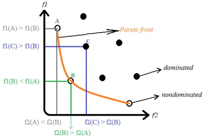
Figure 2.5. Visualization of a two objective space f1 and f2 for a minimization
problem ... 41
Figure 3.1. The representation of individuals ... 46
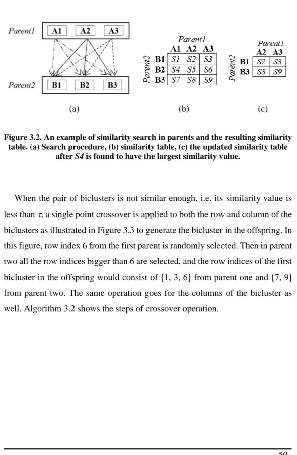
Figure 3.2. An example of similarity search in parents and the resulting similarity table. (a) Search procedure, (b) similarity table, (c) the updated similarity table after S4 is found to have the largest similarity value. ... 50
Figure 3.3. Single-point crossover ... 51
Figure 3.4. The fitness assignment scheme (the strength value and the raw fitness value) for a minimization problem with two objectives f1 and f2 ... 56
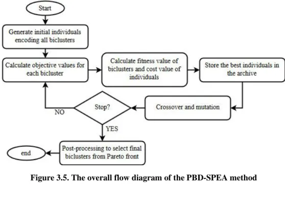
Figure 3.5. The overall flow diagram of the PBD-SPEA method ... 57
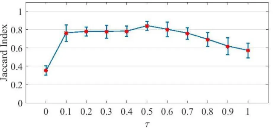
Figure 3.6. Biclustering accuracy for different values of (a) α, (b) β, and (c) τ. Vertical lines are the standard error bars... 62
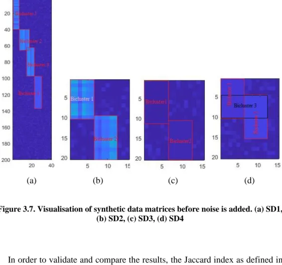
Figure 3.7. Visualisation of synthetic data matrices before noise is added. (a) SD1, (b) SD2, (c) SD3, (d) SD4... 63
xii Figure 3.8. Biclustering accuracy in detecting different biclusters for SD1 data matrix ... 64
Figure 3.9. Biclustering accuracy against different noise level for SD2 data matrix ... 65
Figure 3.10. Biclustering accuracy against different noise level for SD3 data matrix ... 66
Figure 3.11. Biclustering accuracy in detecting different biclusters for SD4 data matrix ... 66
Figure 3.12. Detected biclusters group images with similar concepts ... 75
Figure 3.13. The histogram of the mean values of pairwise cosine distance for randomly generated biclusters (a) network ID 1, (b) network ID 2, (c) network ID 3, (d) network ID 4, (e) network ID 5, (f) network ID 6, (g) network ID 7, (h) network ID 8, (i) network ID 9, (j) network ID 10 ... 80
Figure 4.1. The individual representation ... 85
Figure 4.2. Least square problem; (a) Fitting 2 dimension points to a line, (b) Fitting 3 dimension points to a plane ... 89
Figure 4.3. Visualisation of a 3×2 matrix transformation of rank two, using SVD (Tomasi, 2013) ... 91
Figure 4.4. Local and global optima solutions in a multimodal function ... 93
Figure 4.5. The division of Pareto front into three regions after applying the k-means algorithm when k = 3 ... 95
Figure 4.6. The overall flow diagram of the LBDP method ... 96
Figure 4.7. The accuracy of LBDP (y-axis) considering different parameter values (x-axis). (a) changing all parameter values at the same time to the same value (b) αrr (c) αrc (d) αar (e) αac (f) the number of rows and columns to be
removed and/or added from/to a bicluster ... 101
Figure 4.8. Boxplot of the accuracy (y-axes) for five different data matrices against different noise levels (x-axes) (a) constant value pattern data matrix, (b) constant row pattern data matrix, (c) constant column pattern data matrix, (d) additive pattern data matrix, (e) linear pattern data matrix ... 103
Figure 4.9. The accuracy of the detected biclusters (y-axis) against different noise level (x-axis) (a) constant value pattern data matrix, (b) constant row
xiii pattern data matrix, (c) constant column pattern data matrix, (d) additive pattern data matrix, (e) Linear pattern data matrix... 105
Figure 4.10. The accuracy (y-axis) of detecting different patterns in a data matrix (a) without noise, (b) with Gaussian noise variance 0.3 ... 107
Figure 4.11. The computational time of LBDP (y-axis (ms)) against the dimension of data matrix (x-axis) ... 108
Figure 4.12. The accuracy of the detected biclusters (y-axis) against different dimension (x-axis) data matrices (a) linear pattern bicluster, (b) additive pattern bicluster, (c) the overall accuracy of the methods... 110
Figure 4.13. The accuracy of detected biclusters (y-axis) against the level of overlap (x-axis) ... 111
Figure 4.14. The accuracy of the detected biclusters in the overlapped, noisy data matrix ... 112
Figure 4.15. Number of genes in concurrent annotations including GO terms and KEGG pathways in (a) human Medulloblastoma Tumour (b) Brain Tumour 119
Figure 4.16. Biological enrichment (y-axis (%)) of detected biclusters against different GO annotation level (x-axis) ... 120
xiv List of Tables
Table 2.1. Biomedical databases features ... 11
Table 2.2. A summary of different biclustering techniques ... 19
Table 3.1. The effects of the parameters on the method’s performance ... 59
Table 3.2. The comparison of biclusters of different methods for Yeast and human b-cell data matrices... 67
Table 3.3. Biological process ontology of GOTermFinder ... 68
Table 3.4. Molecular function ontology of GOTermFinder ... 69
Table 3.5. Cellular component ontology of GOTermFinder... 70
Table 3.6. Singular enrichment analysis of KEGG pathway ... 72
Table 3.7. Biclustering results on 10 different Facebook network ... 78
Table 4.1. The effects of the parameters on the method’s performance ... 98
Table 4.2. Data matrices description ... 112
Table 4.3. Statistics of the 100 detected biclusters by LBDP on the Yeast dataset ... 113
Table 4.4. Modular Enrichment Analysis (GO and KEGG Annotation) ... 114
Table 4.5. Cellular Component Ontology ... 114
Table 4.6. Biological Process Ontology ... 115
Table 4.7. Molecular Function Ontology ... 115
Table 4.8. Singular Enrichment Analysis of KEGG Pathway ... 115
Table 4.9. The biclusters of 19 organs detected by LBDP and their GO term116 Table 4.10. The biological enrichment of the breast cancer ... 121
1
Introduction
This thesis presents a multi-objective evolutionary algorithm to solve the biclustering problem in data mining and data analytic communities especially in the field of gene expression data analysis. The challenge of finding biclusters in data matrices is an NP-complete problem (Cheng and Church, 2000) because the search space for finding biclusters increases exponentially when the volume of data increases.
In this chapter, we introduce common data mining method and their shortcomings to uncover interesting patterns in data. Then, we illustrate the methodologies, the aims, and the achievements of this research in terms of the scientific contributions to solve the biclustering problem. Finally, we outline the organisation of the thesis.
1.1 From Clustering to Biclustering
Pattern recognition focuses on finding patterns and regularities in a given data. Extracting interesting patterns in data is an optimization problem (Han et al., 2011). Mining query optimization, performance and pattern evaluation are major issues in data mining (Han et al., 2011) especially when the data tends to be noisy (Fan et al., 2014). Data mining uses a variety of methodologies for analysing and modelling data. It aims at revealing similarity in samples of data while discarding irrelevant samples. A common approach for pattern recognition
2 and data analysis is cluster analysis (Bailey, 1994). Clustering is the task of partitioning samples or features into set of clusters in such a way that elements inside a cluster are more similar while elements from different clusters have low similarity to each other. Traditional clustering approaches such as partitional clustering (Celebi, 2014), hierarchical clustering (Szeto et al., 2003), and density based clustering (Kriegel et al., 2011) have several limitations. For examples, the entire set of features are considered in a cluster. In addition, most clustering methods assign a given sample or feature to only one cluster. However, in many real world situations, a set of samples exhibit similar patterns only under a subset of features (Zhao et al., 2012). Moreover, some samples or features may participate in several clusters and some samples or features may not be part of any cluster.
Given the above, Hartigan introduced biclustering (also called co-clustering) in 1972 and called it direct clustering (Hartigan, 1972) and the term is used in the book of Mirkin (Mirkin, 1996). Biclustering is a data mining method that refers to the clustering of both the sample and feature dimensions in a dataset simultaneously, and it finds subgroups to discover the interrelationship and local patterns from data. In biclustering, a sample can take part in several biclusters under different subsets of features. A bicluster determines a subgroup of elements in the dataset with rearranged samples and features that follow a coherent pattern such that subset of samples shows considerable homogeneity within a subset of features.
To illustrate the differences between clustering and biclustering, Figure 1.1 provides a visualization. Figure 1.1 (a) shows a dataset with 200 samples and 100 features, which contains two biclusters. Figure 1.1 (b) and Figure 1.1 (c) show the element values of the detected clusters by a clustering method and Figure 1.1 (d) and Figure 1.1 (e) show the element values of the detected
3 biclusters by a biclustering method. In Figure 1.1 (b), (c), (d) and (e), the x-axis is the column indices that the methods detected in the clusters or biclusters and the y-axis is the element values. Each line in the plots refers to a sample’s feature vector under a subset of features. Figure 1.1 (b) and (d), and Figure 1.1 (c) and (e) refer to a same set of samples with different subset of features (Figure 1.1 (b) and (c) include all features in the data while Figure 1.1 (d) and (e) include only a subset of features). As can be seen, Figure 1.1 (d) and (e) (i.e. biclusters) display the same pattern i.e. all samples in the detected bicluster exhibit high coherence and can provide more accurate and valuable information about the data.
4
(b) (c)
(d) (e)
Figure 1.1. Conceptual difference of clustering methods (b) and (c) versus biclustering methods (d) and (e), original data matrix is shown in (a) with two
embedded biclusters.
1.2 Research Aims
In this section, we present the problem statement and motivating factors that encouraged us to conduct this research; the aims and the goals we set for this research; the methods of dealing with the research aims to achieve our goals; and our achievements towards the goals and the contributions to the area of research.
5
1.2.1 Problem Statement
In the field of biclustering, the dimension of data, i.e. the number of columns, heavily effects the computational cost of a method. In addition, there exist only a couple of methods (Zhao et al., 2008, Gan et al., 2008) which can handle different type of patterns in noisy data. Furthermore, allowing overlap in biclusters can provide a better representation of information in many real world applications, for example, in the study of the biological relationship between genes and functions in gene expression data. These three factors motivated us to define the main problem of this research. The biclustering problem can be expressed as solving a hyperplane detection problem using a multi-objective evolutionary algorithm.
1.2.2 Research Methodology
Previous studies (Divina and Aguilar, 2006, Golchin and Liew, 2017, Liew, 2016, Mitra and Banka, 2006, Seridi et al., 2011) have shown that one way to enhance the biclustering accuracy is to optimize a fitness function via some iterative process. One promising approach is through the use of evolutionary algorithm (EA). However, there has not been extensive study in this area. In this study, we tackle issues to enhance the biclustering accuracy by
Proposing a novel dynamic encoding scheme with new crossover and mutation operators, which can optimize several biclusters concurrently. Using a newly introduced merit function, our algorithms can handle noisy data and detect overlapping biclusters in a dataset.
Proposing a new geometric based multi-objective EA biclustering method, which is able to search for hyperplanes in a high dimensional feature space.
6 Finding a set of final biclusters from the optimal set of individuals that
constitute the Pareto front in a multi-objective optimization process.
Investigating the generality of the proposed methods to other non-medical datasets such as image data and social media data
1.2.3 Contributions
The focus of this research is to propose methods that are able to discover different bicluster patterns in high dimensional noisy datasets especially gene expression data. Our contributions are as follows.
We proposed two algorithms that are based on multi-objective evolutionary optimization and the geometric biclustering framework.
We developed an effective method to detect hyperplane using SVD during EA optimization.
Our algorithms are able to detect biological meaningful biclusters in noisy and high dimensional data.
Our algorithms can extract overlapped biclusters better than existing algorithms.
Our algorithms can detect different types of bicluster patterns via the geometrical biclustering framework.
1.3 Organization of This Thesis
The rest of this thesis is organised as follows. In the second chapter, a critical survey of the literature and state of art methods has been performed to the biclustering problem. We also discuss their merits and their shortcomings.
7 In Chapter 2, we introduce the biomedical data used in this research, discuss the biclustering problem, the multi-objective evolutionary optimization, and the relevant background knowledge that lead to the proposed methods.
In Chapter 3, we present the first proposed EA based method, called PBD-SPEA (parallel bicluster detection using strength Pareto front algorithm), to search for multiple biclusters concurrently using a novel encoding scheme, crossover operation, and mutation operation.
In Chapter 4, we present our second proposed EA method based on the geometrical biclustering framework, called LBDP (linear bicluster detection by projection). In this method, the hyperplane can be detected effectively using SVD. We also combined niching method to LBDP to search different areas of the multi-objective space simultaneously for multiple bicluster detection.
Finally, in Chapter 5, we sum up this thesis by presenting the conclusions of our research and outline potential future research directions.
8
Background and Literature Survey
During the past couple of decades, a wide range of approaches has been proposed to solve the biclustering problem (Madeira and Oliveira, 2004, Zhao et al., 2012,
Pontes et al., 2015, Padilha and Campello, 2017). Among these approaches, evolutionary methods and geometric methods have attained promising results for the biclustering problem.
In this chapter, we will first discuss biomedical data analysis, specifically that of gene expression data. Second, we will discuss bicluster analysis including the types of bicluster patterns, and validation methods. Then we will review different approaches to address the biclustering problem and highlight their advantages and disadvantages. Finally, the theory of evolutionary algorithm in single objective optimization and multi-objective optimization will be explained.
2.1 Biomedical Data Analysis
Microarrays, also called microscope DNA chips or gene chips, are a collection of DNA (Deoxyribonucleic acid) sequence, known as probes or gene in defined positions attached to a solid surface. A microarray monitors the expression level of thousands of gene samples simultaneously under various biological conditions or at the same time phases in experimental molecular biology (Selvaraj and Natarajan, 2011). The probes, which detect gene expression, are also known as the set of messenger RNA (mRNA).
9 Microarray technologies provide insight about the biological processes at the genomic level enabling the quantitative analysis of gene functions. In microarray analysis, mRNAs are collected from an experimental sample (an individual with a disease like cancer or a treatment) and a reference sample (a healthy individual). Then these two samples are converted into complementary DNA (cDNA) and samples are labeled with different fluorescent colors (usually green and red). The two samples are then mixed and bind to a microarray slide (hybridization). Following hybridization, the expression of each printed gene on the slide is measured. If the expression of a gene is higher in the experimental sample, the corresponding spot in the microarray appears red. This spot appears green otherwise. If there is an equal expression, then the spot appears yellow (Babu, 2004). Figure 2.1 illustrates an overview of the above procedure.
10 Figure 2.1. Microarray procedure. Figure is from
http://ib.bioninja.com.au/standard-level/topic-3-genetics/35-genetic-modification-and/cdna-and-microarrays.html
A gene expression is created by the process of transcribing the genetic information in DNA into mRNA. In the same way, the logarithmic ratios between the intensities of the dyes after some post processing give rise to the gene expression matrix. Ultimately, the data through microarrays that creates the gene expression profiles are used to study the change in the expression of genes in response to a particular condition, diseases, treatment, or development stages. There exists different types of microarrays, namely, cDNA, oligonucleotide arrays, photolithography, ink-jet printing, electrochemical synthesis, single-channel arrays, and multiple-single-channel arrays (Adomas et al., 2008). Gene expression analysis can be a major tool for identifying biomarkers, classifying
11 diseases, monitoring the response to a therapy, diagnosis and prognosis of diseases, and the study of new medicine (Tarca et al., 2006).
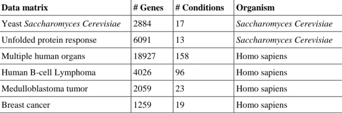
In this research, we are interested in the biclustering of gene expression data where the aim is to infer the biological roles and processes of an unknown gene and unknown genetic pathway by association with known annotated genes in a bicluster (Liew, 2016). Biclustering is also used in the detection of marker genes that are associated with certain tissue, treatment or disease when their expression values are changed (MacDonald et al., 2001, Cha et al., 2014). We used six different gene expression data in our research and an overview of each gene expression dataset is given below. Table 2.1 summarises the main features of the biomedical databases.
Table 2.1. Biomedical databases features
Data matrix # Genes # Conditions Organism
Yeast Saccharomyces Cerevisiae 2884 17 Saccharomyces Cerevisiae
Unfolded protein response 6091 13 Saccharomyces Cerevisiae
Multiple human organs 18927 158 Homo sapiens
Human B-cell Lymphoma 4026 96 Homo sapiens
Medulloblastoma tumor 2059 23 Homo sapiens
Breast cancer 1259 19 Homo sapiens
2.1.1 Yeast Saccharomyces Cerevisiae Database
The yeast Saccharomyces cerevisiae gene expression data (Cho et al., 1998) is one of the most intensively studied dataset in molecular and cell biology. There are many important proteins in common between yeast and human biology. In 60-70% of patients with Crohn’s disease and 10-15% of patients with ulcerative
12 colitis, the antibodies against s. cerevisiae are found (Walker et al., 2004). s. cerevisiae is a significant tool to study DNA damage and repair mechanisms (Nickoloff and Haber, 2001). For this reason, we used this database to study the effectiveness of the proposed methods.
2.1.2 Unfolded Protein Response Database
Unfolded protein response (GDS750) in saccharomyces cerevisiae is the HAC1 transcription and unfolded protein response that strains the expression of HAC1 under various promoters (Leber et al., 2004). There are unrecognized pathways that operates in yeast to regulate the transcription of HAC1. Biclustering aims to distinguish these pathways.
2.1.3 Multiple Human Organs Database
Multiple human organs (Son et al., 2005) originally includes 42421 genes and 158 conditions with 18927 unique genes and 19 different organs. This database helps to understand the cause of diseased organs. Studying this database can help to develop the new targeted genes that can be used in the treatment of patients.
2.1.4 Human B-cell Lymphoma Database
Diffuse large B-cell lymphoma database (Alizadeh et al., 2000) is from an aggressive malignancy of mature B-lymphocytes. Human B-cell lymphoma has attracted lots of attention in the past two decades because over 25000 new cases are obtained annually (Alizadeh et al., 2000). However, most attempts to generate diagnostic solutions failed. Consequently, there is a need to study human B-cell lymphoma in a genomic scale gene expression profiling.
13
2.1.5 Medulloblastoma Tumor Database
Medulloblastoma tumor database (GDS232) is a study on Medulloblastoma metastasis that identifies genes causing medulloblastoma tumors to metastasize (MacDonald et al., 2001). Twenty-three primaries medulloblastoma are analyzed and designated as either metastatic or non-metastatic and 85 genes have already been identified where their expression differs highly from one class to another. Little is known about the genetic regulation in metastatic medulloblastoma and this leads to poor outcomes. Therefore, new methods are needed to study this database.
2.1.6 Breast Cancer Database
Breast cancer database (GDS4085) is from estrogen receptorpositive and -negative breast cancer tumors that analyses the primary breast carcinoma tumors from estrogen receptor positive or negative (ER+/-) patients. ER+ tumors tend to metastasize to the bone while ER- tumors tend to induce visceral metastasis. Nine conditions represent positive tumor and ten conditions represents negative tumor are in this database (Julien et al., 2011). Studying this database provide insight into the molecular basis of different metastatic phenotypes in breast cancer.
2.2 Bicluster Analysis
Let Data = (eij)M×N be a data matrix representing the values of M rows (samples)
denoted by S = {s1, s2, …, sM}, and N columns (N-dimensional feature vector)
denoted by F = {f1, f2, …, fN}. The matrix element eij is the ith row value under
14 Figure 2.2. Data representation
Generally, a bicluster is a subset of rows that exhibit similar behaviour across a subset of columns. Therefore, a bicluster Bic = (R,C) Data exhibits some coherent pattern, where R = {s1, …, sm} S and C = {f1, …, fn} F.
Biclustering aims to discover a set of biclusters such that each bicluster satisfies certain coherent pattern. There are different types of coherent pattern in a bicluster (Cheng et al., 2008). The most common patterns are highlighted here.
Constant value pattern has constant value in the entire pattern as shown in Figure 2.3 (b), which can be represented as ck = … = cj = a1. Constant row pattern
has constant value for each row as in Figure 2.3 (c), which satisfies ck = … = cj.
Constant column pattern has constant value for each column as in Figure 2.3 (d) that corresponds to ck = b1 and cj = b2. Linear pattern has values that satisfies ck
= a2 × cj + b3 as in Figure 2.3 (e). Additive pattern has additive values that
satisfies ck = cj + b4 as in Figure 2.3 (f). Multiplicative pattern has multiplicative
values that satisfies ck = a3 × cj as in Figure 2.3 (g). where a1, a2, a3, b1, b2, b3,
15 Figure 2.3. (a) A 9 × 9 data matrix with hidden biclusters; (b) a constant value
pattern bicluster; (c) a constant row pattern bicluster; (d) a constant column pattern bicluster; (e) a linear pattern bicluster; (f) an additive pattern bicluster;
(g) a multiplicative pattern bicluster
From the geometrical viewpoint, we can consider each pattern as a special case of linear pattern ck = A × cj + B, i.e. in constant value pattern, A = 0 and B
= a; in constant row pattern, A = 1 and B = 0; in constant column pattern, A = 0; in additive pattern, A = 1; in multiplicative pattern, B = 0, where A and B are constant values.
16 Given the above, if the columns are considered as coordinate axes in a high-dimensional space, a constant value pattern and constant column pattern form a point, constant row pattern forms a line, whereas additive pattern, multiplicative pattern, and linear pattern form a hyperplane in the space.
The geometric interpretation of linear bicluster patterns unifies all bicluster patterns into a single linear class and allows a unified treatment in detecting them simultaneously (Du et al., 2014). This is in contrast to most existing biclustering methods where the cost function implicitly imposes a constraint on the type of bicluster patterns that could be discovered.
In principle, any method for detecting linear patterns i.e. hyperplane detection methods, can be employed to detect biclusters in data matrices. This characteristic of linear patterns is the basis of the geometric biclustering frameworks.
The other challenging issue in biclustering is how to validate a detected bicluster. Validating the quality of biclusters is accomplished by using measures derived from the data itself or by using domain knowledge (Zhao et al., 2012).
We can compute some quality measures of a biclustering result to evaluate the accuracy of the detected biclusters when the true biclusters are known in the data such as in synthetic data. In this case, Jaccard index, also called matching score, counts the number of rows and columns that are common between the detected bicluster and the ground truth as in Equation (2.1). The value of Jaccard index varies from zero to one where zero indicates no similarity and one indicates 100% similarity. The higher the value of Jaccard index, the better the accuracy of the detected bicluster and ultimately the better the performance of the method. The Jaccard index J is defined by
17 𝐽(𝐵𝑖𝑐, 𝐺) = 1 |𝐵𝑖𝑐|∑ 𝑚𝑎𝑥𝑅𝐺,𝑐𝐺 |𝑅 ∩ 𝑅𝐺| + |𝐶 ∩ 𝐶𝐺| |𝑅 ∪ 𝑅𝐺| + |𝐶 ∪ 𝐶𝐺| 𝑅,𝐶 (2.1)
where G is the bicluster ground truth, RG and CG are rows and columns of the
bicluster ground truth. |•| represents the number of elements. J calculates the ratio of similar rows and columns over the total number of rows and columns in the detected bicluster and the ground truth.
Gene expression data measures the expression level of thousands of genes (rows) under various biological conditions (columns). For gene expression analysis, the domain knowledge about the gene expression data helps to assess the biological relationship of the detected genes and enables the quantitative analysis of genes. A common way to check the enrichment in the biclusters is by using p-value statistics. The p-value measures the probability of finding the number of genes with a specific GO term in a bicluster by chance and shows the statistical significance of the results. Smaller p-value indicates strong evidence that the selected genes are highly correlated. Equation (2.2) calculates the p-value, where A is the number of annotated genes in the background set, and k is the number of annotated genes within the detected genes.
𝑃 = 1 − ∑(𝐴𝑖) (𝑀 − 𝐴𝑅 − 𝑖) (𝑀 𝑖) 𝑘−1 𝑖=0 (2.2)
In order to study the biological relevance of extracted biclusters we can use Gene Ontology (GO), metabolic pathway maps (MPM), protein-protein interaction networks (PPI), and Kyoto Encyclopaedia of Genes and Genomes (KEGG) pathway. GO is organized into hierarchical annotations (Ashburner et al., 2000) while the KEGG database organizes the genes products into pathway reaction maps (Kanehisa and Goto, 2000).
18 In addition, KEGG pathway represents the known biological knowledge about the molecular interaction and reaction networks for genetic information processing, cellular process, human diseases, and drug development (Kanehisa and Goto, 2000).
Three ontologies are available in GO which provides a dynamic, controlled vocabulary for various genomic databases, namely, biological process that represents the effects of genes in a biological objective, molecular function that shows biochemical activity, and cellular component, which refers to a location in the cell where a gene product is activated (Ashburner et al., 2000).
Tools such as GeneCodis (Tabas Madrid et al., 2012, Nogales Cadenas et al., 2009, Carmona Saez et al., 2007), GO-TermFinder (Boyle et al., 2004), and ClueGO (Bindea et al., 2009) study the biological relationship of extracted biclusters by analyzing modular and singular enrichment. GeneCodis is available online at http://genecodis.cnb.csic.es/ and calculates the p-value for different annotations. This toolbox also calculates modular enrichment analysis that provides a complete functional analysis by detecting additional significant terms (Mahé et al., 2014).
Depending on the bicluster pattern and the search strategy, a number of biclustering methods have been proposed (Zhao et al., 2012). These include distance based biclustering, spectral based biclustering, probabilistic based biclustering, geometric based biclustering, and evolutionary based biclustering. We will next review the general concepts and several well-known methods in each category. An overview of these methods is summarised in Table 2.2.
19 Table 2.2. A summary of different biclustering techniques
Category Method Reference
Distance based biclustering Iterative greedy search - CC (Cheng and Church, 2000) Spectral based biclustering Eigenvector decomposition of
normalized data
(Kluger et al., 2003)
Factor based coherence optimization by max-sum
(Denitto et al., 2017b)
Two-way subspace partitioning - TWCC
(Chen et al., 2018)
Probabilistic based biclustering
Data decomposition - FABIA (Hochreiter et al., 2010) Data decomposition - SSBiEM (Denitto et al., 2017a) Semantic enrichment (Kléma et al., 2017) Convex optimization - COBRA (Eric et al., 2017) Geometric based biclustering Fast Hough transform (Gan et al., 2005) Column pair Hough transform (Zhao et al., 2008) Column pair Hough transform (Wang and Yan, 2010) Graph spectrum column pair
Hough transform
(Wang et al., 2012)
Graph spectrum column pair Hough transform
(Wang and Yan, 2013)
Graph spectrum column pair Hough transform
(Liu et al., 2014)
Genetic algorithm hyperplane detection
(To and Liew, 2014)
Evolutionary based biclustering
Multi-objective multi-population artificial immune network – MOM-aiNet
(Coelho et al., 2008)
Dynamic multi-objective immune network optimization - DMOIOB
(Liu et al., 2011)
Genetic algorithm optimization (Divina and Aguilar Ruiz, 2006)
Optimal reordering of samples and features - OPSM
(Roh and Park, 2008)
Multi-objective non-dominated sorting genetic algorithm
20
Category Method Reference
Multi-objective genetic optimization (Maulik et al., 2009) Multi-objective evolutionary optimization (Seridi et al., 2011)
2.2.1 Distance based Biclustering
This method is one of the earliest methods in literature and it has applications in many fields. Distance based biclustering measures the quality of the biclusters using a distance metric and an iterative search by adding and/or removing rows or columns such that the residual sum of squares cost is minimized. Among different introduced residual measures, mean square residue (MSR) introduced by (Cheng and Church, 2000) is the most famous one. Although these methods may fail to detect biclusters and mostly cover constant and additive structures only, they have the potential to be very fast (Madeira and Oliveira, 2004).
Cheng and Church (CC) (Cheng and Church, 2000) were the first to apply biclustering method to analyse the biological gene expression data. They used a heuristic greedy search method to detect δ-biclusters one at a time. For a predefined number of biclusters, they iteratively removed and inserted rows and columns to a detected bicluster while the MSR error remained below δ. Some recent evolutionary based methods have used this method as a local search strategy (Golchin and Liew, 2017, Golchin and Liew, 2016, Golchin et al., 2015, Seridi et al., 2012, Seridi et al., 2011).
MSR measures the degree of coherence of a bicluster. Equation (2.3) calculates MSR value where eiC, eRj and eRC are the mean of the ith row, the mean
21 calculated by Equations (2.4)-(2.6). If MSR(R,C) ≤ δ then a bicluster is called a δ-bicluster. The smaller δ is, the better the coherence of the rows and columns.
𝑀𝑆𝑅(𝑅, 𝐶) = (∑ (𝑒𝑖𝑗 − 𝑒𝑖𝐶− 𝑒𝑅𝑗 + 𝑒𝑅𝐶)2 𝑖∈𝑅,𝑗∈𝐶 )/|𝑅||𝐶| (2.3) 𝑒𝑖𝐶 = (∑ 𝑒𝑖𝑗 𝑗∈𝐶 )/|𝐶| (2.4) 𝑒𝑅𝑗 = (∑ 𝑒𝑖𝑗 𝑖∈𝑅 )/|𝑅| (2.5) 𝑒𝑅𝐶 = (∑ 𝑒𝑖𝑗 𝑖∈𝑅,𝑗∈𝐶 )/|𝑅||𝐶| (2.6)
2.2.2 Spectral based Biclustering
In contrast to the methods that apply greedy heuristic search for biclustering problem, spectral based biclustering methods use spectral decomposition techniques. Spectral decomposition uncovers natural structures in the data that are related to hidden biclusters. The main drawback of these methods is the long computation time.
Kluger et al. (Kluger et al., 2003) found distinctive checkerboard structure patterns in the data matrices by eigenvectors corresponding to characteristic patterns across rows or columns. They assumed that the data matrix has a block diagonal structure in a way that elements outside the blocks equal to zero. In this case, each block corresponded to a bicluster. They used singular value decomposition to identify columns with the same conserved linear structure across the rows in a normalized data matrix. The normalization was done with a standard linear algebra manipulation and the whole data matrix was used in a global manner to eliminate the effects of different experimental columns. The
22 authors applied their method to cancer genomic data matrices and they achieved reasonable results.
In (Denitto et al., 2017b), the biclustering problem was solved by performing sequential search for one bicluster at a time. In order to make their proposed method scalable in comparison to the previous factor based (FG) methods, the authors used a compact binary FG based on a given coherence optimization criteria by the max-sum method. In their method, each bicluster was represented as a binary matrix Bic {0,1}n×m where b
ij = 1 if the entry (i,j) belongs to the
bicluster and zero otherwise. They found the largest biclusters by measuring the incoherence of a bicluster as a constant-type incoherence by I(eij,etk) = (eij - etk)2
or an additive-wise incoherence by I(eij,etk) = (eij - etj + etk – eik)2. They also
rewarded the solutions containing entries with high values by assuming that all the entries in a data matrix contained only positive values. Finally, their method tried to maximize the following function, where Aij(bij) = eij if bij = 1 and 0
otherwise, Oij,tk = -I(eij,btk)bijcik, and Bjk(b:j,b:k) = 0 if (ibij)(ibik)(i|bij-bik|) = 0
and - otherwise. 𝐹(𝐶) = ∑ ∑ 𝐴𝑖𝑗(𝑏𝑖𝑗) 𝑛 𝑗=1 𝑚 𝑖=1 + ∑ ∑ ∑ ∑ 𝑂𝑖𝑗,𝑡𝑘(𝑏𝑖𝑗, 𝑏𝑡𝑘) 𝑛 𝑘=1 𝑚 𝑡=1 𝑛 𝑗=1 𝑚 𝑖=1 + ∑ ∑ 𝐵𝑗𝑘(𝑏:𝑗, 𝑏:𝑘) 𝑛 𝑘=1 𝑛 𝑗=1
In their method, they use three types of factors namely, Aij, Oij,tk, and Bjk to
derive six types of messages. The authors tested the accuracy of their method by both synthetic and real dataset and achieved promising results compared to state-of-the-art methods. Although compared to other FG methods, their method has
23 achieved acceptable results, there are tight assumptions that limit their method as summarised in the following.
Using a sequential bicluster detection approach would miss the overlapped area in the detected biclusters. For this reason, in their experiments they used only one bicluster in their synthetic dataset. In addition, to calculate the incoherence of the biclusters they proposed using two models namely additive coherent and constant wise coherent. This assumption makes their method unable to detect the more general type of biclusters with linear structure. Further, they assumed the values of the data matrix are all positive, which is unrealistic for gene expression data. In their paper, the authors mentioned “the entry level counts” and they rewarded biclusters that contain elements with larger value in comparison to the background elements. However, what happen if the element values of a bicluster are close to the background noise?
Most importantly, they demonstrated their method for a 50 × 50 data matrix but in order to scale up, they used a divide and conquer strategy to randomly partition the data matrix into non-overlapping submatrices. In addition, in order to overcome the curse of dimensionality, they ignore a reasonable portion of the data matrix. The authors adopt an affinity propagation method to merge the obtained biclusters in real life datasets. However, this process is time consuming and there is no guarantee to obtain the optimal biclusters.
A two-way subspace weighting partitioned co-clustering method TWCC was proposed in (Chen et al., 2018). Two types of binary weight matrices separate the data matrix into subspaces i.e. columns in row clusters and rows in column clusters. These weights that deal with noisy data, are combined by Hadamard product of the two binary matrices to simultaneously determine the contribution of each row or column in co-clusters. The Bregman block average co-clustering
24 (BBAC) uses a squared Euclidean distance function based on these two types of weights to determine the co-clusters of data, and an iterative algorithm, is used to optimize the distance function.
Equation (2.7) is the objective function that are minimized, where K and L are the number of row clusters and column clusters, respectively. U and V are the two binary matrices, in which uig = 1 indicates that the ith row is assigned to
the gth row cluster and vjh = 1 indicates that the jth column is assigned to the hth
column cluster. Z is the centres of the K×L co-clusters. R and C are the weight matrices for rows and columns, respectively. λ And η are two positive parameters. d(eij, zgh) is the Bregman divergence and is defined as (eij – zgh)2.
The authors had run experiment on both real and synthetic datasets and claimed that their proposed method is robust and effective for large high-dimensional data. 𝑃(𝑈, 𝑉, 𝑍, 𝑅, 𝐶) = 1 𝑀𝑁∑ ∑ ∑ ∑ 𝑢𝑖𝑔𝑣𝑗ℎ𝑟ℎ𝑖𝑐𝑔𝑗𝑑(𝑒𝑖𝑗, 𝑧𝑔ℎ) 𝑁 𝑗=1 𝑀 𝑖=1 𝐿 ℎ=1 𝐾 𝑔=1 + 𝜆 𝑀∑ ∑ 𝑟ℎ𝑖log 𝑟ℎ𝑖 𝑀 𝑖=1 𝐿 ℎ=1 + 𝜂 𝑁∑ ∑ 𝑐𝑔𝑗log 𝑐𝑔𝑗 𝑁 𝑗=1 𝐾 𝑔=1 (2.7)
The performance of TWCC is sensitive to the threshold values of the penalty terms in the objective function. Furthermore, they have no strategy to handle overlapped biclusters which is an important issue in real life data.
2.2.3 Probabilistic based Biclustering
In this category, a probabilistic model of biclusters and statistical parameter estimation techniques is used to search for the biclusters. The idea is that in order to detect the existence of a bicluster, non-deterministic methods are designed
25 that detect a bicluster if the probability of a failure is less than a threshold. Not only these methods are technically complex but also these methods may not detect the desired bicluster (Alon and Spencer, 2004).
Hochreiter et al., (Hochreiter et al., 2010) proposed a generative approach based on a multiplicative model called FABIA (factor analysis for bicluster acquisition). Their method was able to detect linear dependencies between rows and columns and it had been designed for heavy tailed distributions as found in many real world data. The authors decomposed a data matrix in levels and assumed the data was the sum of several biclusters with additive noise, i.e. 𝐷𝑎𝑡𝑎 = ∑𝑝𝑖=1𝜆𝑖𝑧𝑖𝑇 + 𝛶 = 𝛬𝛧 + 𝛶, where Λi RM and zi RN are the sparse
vectors corresponding to the ith bicluster, ϒ Rn×m is the additive noise. Despite of using variational expectation maximization to estimate the model parameters, the corresponding likelihood is not tractable. Further, a post-processing step is needed to provide the biclusters membership information.
Following the work of (Hochreiter et al., 2010) and in order to overcome the drawbacks of their models, in (Denitto et al., 2017a) the authors addressed the problem of biclustering by approaching it as a probabilistic sparse low-rank matrix factorization problem. They designed a probabilistic model to describe the factorization of a given data matrix into the product of two matrices that
provided the rows and columns of the biclusters, i.e. 𝐷𝑎𝑡𝑎 = ∑𝑘𝑖=1𝑣𝑖𝑧𝑖𝑇+ 𝑌 = 𝑉𝑍 + 𝑌, where Y is random noise. Each bicluster had its own parameter values and is the outer product of two sparse vectors, with the data matrix being modelled as the sum of k (number of biclusters which is known beforehand) outer products (VZ). The authors modelled the data as a Gaussian distribution having VZ as mean and the estimated noise as the variance, and used a spike and slab sparsity inducing prior (SSBi).
26 Spike and slab is a probabilistic model for variable selection. In order to estimate the model parameters and bicluster membership information, expectation-maximization (EM) method was proposed (SSBiEM) to solve the problem of low-rank factorization problem by the augmented Lagrangian method.
The main ingredient of their method is that they assumed the vectors corresponded to the biclusters are sparse. This is a drawback since sometimes a bicluster can be a big part of the original data matrix. The EM method proposed in their paper involves an approximate M-step that minimizes a non-convex function and there is no guarantee that the method will converge. Furthermore, the performance may depend on the initialization step. The authors also claimed that their methods allows for overlapped biclusters. We tested their method (available online at https://github.com/emme-di/ssbiem/) with the data matrix designed in Experiment 4 of Section 4.3.2. The Jaccard index is 0.94 when there is no overlapped in the data matrix, but the performance drops significantly when the overlapped degree increases.
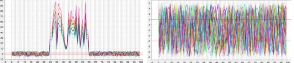
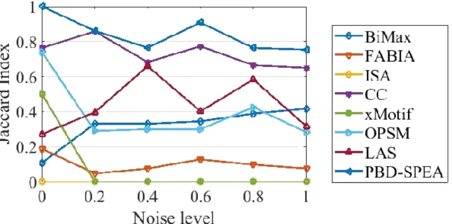
27 Figure 2.4. The accuracy of detected biclusters in (Denitto et al., 2017a) when the
level of overlapped is 2
As can be seen from Figure 2.4, SSBiEM (Denitto et al., 2017a) detects both biclusters as one bicluster including the overlapped rows and columns and a second bicluster excluding the overlapped rows and columns.
(Kléma et al., 2017) proposed a method called semantic biclustering to detect interpretable rectangular patterns in binary data matrices. To do so, they used an existing biclustering method with the semantic ingredient i.e. enrichment, and a rule and tree learning machine learning. The authors assumed a joint probability distribution over a set of rows, a set of columns, and a binary set of expression indices. In order to test the quality of their biclusters, they counted the number of ones inside a bicluster and zeros outside of it as (i,j)ext(B) eij + (i,j)M×N\ext(B)
1-eij , where ext(B) = {(i,j): im, jn, (m,n)B} and B = {Bic}. They tested their
methods on two real gene expression data and they indicated that the biclustering enrichment method achieves the best performance.
28 (Eric et al., 2017) presented a simple and interpretable convex optimization
formulation of the biclustering that possessed a unique global minimizer (F(U)) and a penalized regression (J(U)) problem. The minimizer is assumed to be continuous in the data. In their method, called COBRA, a single tunning parameter that controlled the number of biclusters, was generated that included an entire solution path of possible biclusters. In order to regenerate their results, COBRA always mapped data to a single biclustering assignment. Each element of the data matrix was assumed to be eij = 0 + rc + ij, where 0 is the grand
mean shared by all elements and is equal to zero to model a checkerboard mean for the biclustering problem. rc = 1/(|R||C|)iR,jC eij, is the mean of the
bicluster, and ij is assumed to be an independent and identical distribution
N(0,2) for some 2 > 0. The partitions were identified by minimizing the following convex function:
𝐹𝛾(𝑈) = 1 2‖𝐷𝑎𝑡𝑎 − 𝑈 ‖2𝐹+ 𝛾[Ω⏟ 𝑊(𝑈) + Ω𝑊̃(𝑈𝑇)] 𝐽(𝑈) , Ω𝑊(𝑈) = ∑ ‖𝑈.𝑖− 𝑈𝑗.‖2 𝑖<𝑗
where U.i (Ui.) denotes the ith column (row) of the matrix U and U is the estimate
of the mean matrix . J(U) penalizes deviations away from a checkerboard pattern and 0 tunes the two terms. COBRA was considered as a principled reformulation of the clustered dendrogram. They showed the stability and reproducibility of biclustering on both simulated and real microarray data. However, their method was not applicable for overlapped biclusters.
29
2.2.4 Geometric based Biclustering
Geometric biclustering method is a recently introduced biclustering method based on transferring the element values of a data matrix to a higher dimensional space (Zhao et al., 2008, Gan et al., 2008, To and Liew, 2014). In this method, each column corresponds to a dimension in a higher dimensional space and the rows correspond to points in this higher dimensional space. Thus, different patterns of linear biclusters can be categorised as points, lines or hyperplanes in the new dimensional space.
(Liu et al., 2014, Wang and Yan, 2013, Wang et al., 2012, Wang and Yan, 2010, Zhao et al., 2008, Gan et al., 2005) considered the geometrical viewpoint of biclustering, i.e. hyperplane detection, leading to finding linear pattern biclusters in the data matrices. In computer vision, an effective way to detect linear structures is Hough transform (HT) (Hough, 1962, Hough, 1959). HT identifies lines in the data matrix by a voting procedure in Hough space. HT maps the x-y coordinates into ρ-θ parameter space where ρ is the distance of the line to the origin and θ is the angle of the normal vector with the x-axis. HT parametrizes the pattern space then projects all points into the parameter space, from which the local maxima in an accumulator implies the existence of line candidates.
Gan et al. (Gan et al., 2005) proposed to detect biclusters in two main steps. First, they detected a bundle of hyperplanes among a data matrix using fast Hough transform method. Then they analysed the detected planes to see whether the planes contain any coherent values by additive and multiplicative models. They used synthetic data matrices to validate their results.
Generally, HT is computationally expensive and the storage memory requirement is high. This makes HT un-scalable for high dimensional data, thus,
30 Zhao et al., (Zhao et al., 2008) applied Hough transform in a column pair space. The authors developed a visualization tool, additive and multiplicative pattern plot (AMPP), to figure out the collinear points and to classify points into additive and multiplicative patterns. The intersection of the rows and the union of the columns generated the maximal biclusters. In their method, they detected different types of biclusters one by one.
Wang and Yan (Wang and Yan, 2010) also applied Hough transform in column pair space to find biclusters. A hypergraph model merged the sub-biclusters to generate larger sub-biclusters. In (Wang et al., 2012, Wang and Yan, 2013, Liu et al., 2014), the authors extended their method and they built their graph regarding each Hough vector as a node. The graph spectrum is utilized to produce larger biclusters.
All these efforts in using HT show the effectiveness of HT in detecting biclusters. However, the heuristic combination strategies may fail with regard to detect and combine sub-biclusters to generate bigger biclusters and may converge to a local maximum.
In order to overcome the space usage and complexity of HT, evolutionary algorithms (EA) and heuristic search are introduced into the geometric biclustering (To and Liew, 2014).
In (To and Liew, 2014), To and Liew combined genetic algorithms (GA) and the steepest descent to obtain the parameters of the fittest hyperplane. In their method, the fitness function was the root mean square error (RMSE) of the hyperplane. However, using steepest descent for parameter selection of the hyperplane was very time consuming.
31 The algorithms based on geometric based biclustering are not only able to detect all types of linear biclusters but can also handle overlapping biclusters. However, the use of HT makes these methods not scalable and the heuristics based on divide-and-conquer may fail to detect maximal biclusters.
2.2.5 Evolutionary based Biclustering
Evolutionary algorithm (EA) is a popular metaheuristic method for global optimization because of its excellence ability to explore a search space and to solve complex problems (De Jong, 2006). Using evolutionary-based approaches to solve the biclustering problem especially in gene expression data analysis has attracted tremendous attention after the seminal work of Cheng and Church in 2000 (Cheng and Church, 2000). Hence, researchers have proposed to apply evolutionary algorithms as a search strategy to the biclustering problem (Golchin and Liew, 2017, Liew, 2016, Golchin and Liew, 2016, Golchin et al., 2015, Pontes et al., 2013, Seridi et al., 2011, Roh and Park, 2008, Mitra and Banka, 2006, Divina and Aguilar Ruiz, 2006). Depending on the fitness function defined in EA, these methods can detect all types of biclusters. EA search strategy includes artificial immune system (AIS) and genetic algorithms (GA).
2.2.5.1 AIS based Biclustering
Artificial immune system (AIS) is a subfield of evolutionary algorithms inspired by the biological immune system. The methods in artificial immune system can be classified into clonal selection method, negative selection method, immune network method, and dendritic cell method (De Castro and Timmis, 2002).
In (Coelho et al., 2008), the authors used artificial immune network to search for multiple biclusters concurrently. In their proposed method, called multi-objective multi-population artificial immune network (MOM-aiNet), they
32 minimized the MSR and maximized the bicluster volume through multi-objective search. To detect multiple biclusters concurrently, the authors generated a subpopulation for each bicluster by randomly choosing one row and one column of the data matrix and running the multi-objective search on each subpopulation separately. In each iteration, each subpopulation underwent cloning and mutation. Then, all non-dominated biclusters was used to generate the new population for the next iteration. The method aimed to converge to distinct regions of the search space. To do this, MOM-aiNet compared the degree of overlap of the largest biclusters of each population. If the overlap value was greater than a threshold, two subpopulations were merged to a single subpopulation. The method also generated new random subpopulations from time to time.
Liu et al (Liu et al., 2011) proposed a dynamic multi-objective immune optimization biclustering method (DMOIOB). They detected maximized biclusters with minimized MSR and maximized row variance. A binary string encoded the antibodies of a fixed number of rows and a fixed number of columns. Their method started by generating antibodies population and antigen population. Then the size of the antibodies population increased to ensure a sufficient number of individuals and to explore unvisited areas of the search space. For each antibody, best local guide was selected using Sigma method and the best antibodies were used to produce the next generation. Non-dominated individuals were used to update the antigens population. Moreover, the size of the antibodies population was decreased to prevent excessive growth in population. In order to find the local best solution, they applied the basic idea of Sigma method and immune clonal selection among the archive individuals. The quality of the objective values and a biological analysis of the biclusters were
33 used to validate their method. DMOIOB achieved the diversity of solutions by
using the concept of crowding distance and -distance.
However, using only these distances do not guarantee diversity among archive individuals. For example, if there are two biclusters in a data matrix with the same volume and the same values, then these biclusters have the same objective values in the objective space and the method ignores one of them.
2.2.5.2 GA based Biclustering
Genetic algorithm is a subfield of evolutionary algorithms inspired by natural evolution to generate reliable solutions to optimization problems and search problems by relying on mutation, crossover, and selection. In a genetic algorithm, a population of solutions evolve toward better solutions over several generations. Each solution has a set of properties encoded as a binary string or other encoding schemes.
Divina and Aguilar-Ruiz (Divina and Aguilar Ruiz, 2006) proposed an evolutionary computation method that combined the bicluster size, MSR, and row variance in a single objective cost function. In their method, the authors found biclusters with bigger size, higher row variance, smaller MSR and low level of overlapping among biclusters. They used Equation (2.3) to calculate MSR value and Equation (2.8) to calculate row variance of bicluster Bic = (R,C).
𝑣𝑎𝑟𝑅𝐶 = (∑ (𝑒𝑖𝑗− 𝑒𝑖𝐶)2
𝑖∈𝑅,𝑗∈𝐶 )/|𝑅||𝐶| (2.8)
In order to avoid overlapping, the authors used a penalty value as the sum of
weight matrix associated with the expression matrix (penalty = wp(eij)). The