Forecasting Models for Integration of Large-Scale Renewable Energy Generation to Electric Power Systems

(1)

A Thesis Submitted to the College of Graduate and Postdoctoral Studies In Partial Fulfillment of the Requirements

For the Degree of Doctor of Philosophy

In the Department of Electrical and Computer Engineering University of Saskatchewan

Saskatoon

By

Nima Safari

(2)

i

PERMISSION TO USE

In presenting this thesis in partial fulfillment of the requirements for a Postgraduate degree from the University of Saskatchewan, I agree that the Libraries of this University may make it freely available for inspection. I further agree that permission for copying of this thesis/dissertation in any manner, in whole or in part, for scholarly purposes may be granted by the professor or professors who supervised my thesis/dissertation work or, in their absence, by the Head of the Department or the Dean of the College in which my thesis work was done. It is understood that any copying or publication or use of this thesis or parts thereof for financial gain shall not be allowed without my written permission. It is also understood that due recognition shall be given to me and to the University of Saskatchewan in any scholarly use which may be made of any material in my thesis.

Requests for permission to copy or to make other uses of materials in this thesis/dissertation in whole or part should be addressed to:

Head of the Department of Electrical and Computer Engineering 57 Campus Drive

University of Saskatchewan Saskatoon, Saskatchewan (S7N 5A9)

Canada OR

Dean

College of Graduate and Postdoctoral Studies University of Saskatchewan

116 Thorvaldson Building, 110 Science Place Saskatoon, Saskatchewan (S7N 5C9)

(3)

ii

ABSTRACT

Amid growing concerns about climate change and non-renewable energy sources depletion, variable renewable energy sources (VRESs) are considered as a feasible substitute for conventional environment-polluting fossil fuel-based power plants.

Furthermore, the transition towards clean power systems requires additional transmission capacity. Dynamic thermal line rating (DTLR) is being considered as a potential solution to enhance the current transmission line capacity and omit/postpone transmission system expansion planning, while DTLR is highly dependent on weather variations. With increasing the accommodation of VRESs and application of DTLR, fluctuations and variations thereof impose severe and unprecedented challenges on power systems operation. Therefore, short-term forecasting of large-scale VERSs and DTLR play a crucial role in the electric power system op-eration problems. To this end, this thesis devotes on developing forecasting models for two large-scale VRESs types (i.e., wind and tidal) and DTLR.

Deterministic prediction can be employed for a variety of power system operation problems solved by deterministic optimization. Also, the outcomes of deterministic prediction can be employed for conditional probabilistic prediction, which can be used for modeling uncertainty, used in power system operation problems with robust optimization, chance-constrained optimization, etc. By virtue of the importance of deterministic prediction, deterministic prediction models are developed. Prevalently, time-frequency decomposition approaches are adapted to decompose the wind power time series (TS) into several less non-stationary and non-linear components, which can be predicted more precisely. However, in addition to non-stationarity and nonlinearity, wind power TS demonstrates chaotic characteristics, which reduces the predictability of the wind power TS. In this regard, a wind power generation prediction model based on considering the chaosity of the wind power generation TS is addressed. The model consists of a novel TS decomposition approach, named multi-scale singular spectrum analysis (MSSSA), and least squares support vector machines (LSSVMs).

Furthermore, deterministic tidal TS prediction model is developed. In the proposed prediction model, a variant of empirical mode decomposition (EMD), which alleviates the issues associated with EMD. To further improve the prediction accuracy, the impact of different components of wind power TS with different frequencies (scales) in the spatiotemporal modeling of the wind farm

(4)

iii

is assessed. Consequently, a multiscale spatiotemporal wind power prediction is developed, using information theory-based feature selection, wavelet decomposition, and LSSVM.

Power system operation problems with robust optimization and interval optimization require prediction intervals (PIs) to model the uncertainty of renewables. The advanced PI models are mainly based on non-differentiable and non-convex cost functions, which make the use of heuristic optimization for tuning a large number of unknown parameters of the prediction models inevitable. However, heuristic optimization suffers from several issues (e.g., being trapped in local optima, irreproducibility, etc.). To this end, a new wind power PI (WPPI) model, based on a bi-level optimization structure, is put forward. In the proposed WPPI, the main unknown parameters of the prediction model are globally tuned based on optimizing a convex and differentiable cost function. In line with solving the non-differentiability and non-convexity of PI formulation, an asymmetrically adaptive quantile regression (AAQR) which benefits from a linear formulation is proposed for tidal uncertainty modeling. In the prevalent QR-based PI models, for a specified reliability level, the probabilities of the quantiles are selected symmetrically with respect the median probability. However, it is found that asymmetrical and adaptive selection of quantiles with respect to median can provide more efficient PIs. To make the formulation of AAQR linear, extreme learning machine (ELM) is adapted as the prediction engine. Prevalently, the parameters of activation functions in ELM are selected randomly; while different sets of random values might result in dissimilar prediction accuracy. To this end, a heuristic optimization is devised to tune the parameters of the activation functions.

Also, to enhance the accuracy of probabilistic DTLR, consideration of latent variables in DTLR prediction is assessed. It is observed that convective cooling rate can provide informative features for DTLR prediction. Also, to address the high dimensional feature space in DTLR, a DTR prediction based on deep learning and consideration of latent variables is put forward.

Numerical results of this thesis are provided based on realistic data. The simulations confirm the superiority of the proposed models in comparison to traditional benchmark models, as well as the state-of-the-art models.

(5)

iv

ACKNOWLEDGMENTS

First, I would like to express my sincere gratitude to my supervisor Dr. Chi Yung Chung for his continuous support throughout my Ph.D. study. I have learned priceless lessons from his expertise, vision, and personality. He has also financially supported me throughout my Ph.D. program and made it possible to only zero in on my research without any financial concerns.

Also, I would like to thank the College of Graduate and Postdoctoral Studies for providing the Dean’s Scholarship which is the most prestigious scholarship in the University. Besides, I would like to thank the National Science and Engineering Research Council for providing partial financial support. Also, I would like to sincerely thank the Saskatchewan Power Corporation (SaskPower) for providing data. Special thanks go to the members of my advisory committee: Dr. Nurul A. Chowdhury, Dr. Khan Wahid, Dr. Daniel Chen, and Dr. Seok-Bum Ko for their insightful comments and suggestions throughout my Ph.D. program.

The last but not the least, I owe my deepest gratitude to my parents, Mehdi and Zahra, and my loving wife, Elnaz. Words cannot express how grateful I am to them for their continuous spiritual support.

(6)

v

DEDICATION

Dedicated to my Father, Mehdi, my Mother, Zahra,

and

(7)

vi

LIST OF TABLES AND ILLUSTRATIONS

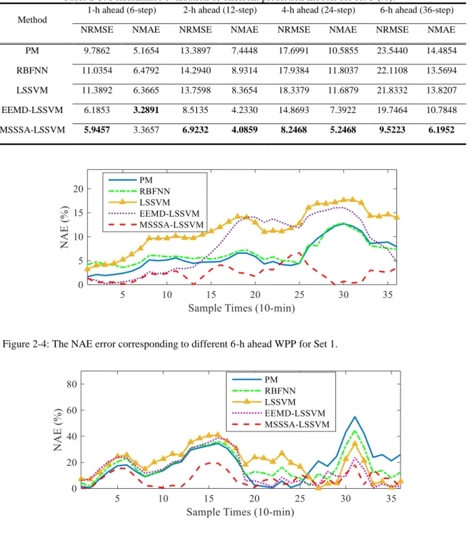
Table 2-1: Performance evaluation of different prediction models for set 1 (%). ... 37

Table 2-4: Percentage of NRMSE and NMAE reduction compared to persistence model ... 41

Table 2-5: Performance comparison of GAM and MSSSA-LSSVM ... 43

Table 3-1: Performance evaluation of different prediction models for 1-h (10-step) ahead TCS prediction ... 57

Table 3-2: Performance evaluation of different prediction models for 1-h (10-step) ahead TCS prediction ... 59

Table 4-1: Performance comparison of different WPP models for Sunbridge wind power facility in July 2016. ... 73

Table 4-2: Performance Comparison of Different WPP Models for Red Lily Wind Power Facility in July 2016. ... 73

Table 5-1: Evaluation of the Proposed WPPI in 1-Step Ahead Prediction for Feb. 2012 and 𝑅𝐿 ∗ = 90%. ... 100

Table 5-2: Performance Evaluation of Different Prediction Models for Various Months in 6-step Ahead Prediction for 𝑅𝐿 ∗= 90% ... 103

Table 5-3: Summary of Performance Evaluation of WPPI Models in 1-Step Ahead for Multi Runs and 𝑅𝐿 ∗= 90% ... 105

Table 5-4: Summary of Computation Time for Training ... 106

Table 5-5: Performance Evaluation of NCWC-based Elman and NARX WPP Models and the Proposed WPPI for Prediction for 𝑅𝐿 ∗= 90% ... 107

(15)

xiv

Table 6-2: Results of 10-minute ahead PI construction of tidal data (Minimum 𝑅𝐿 ∗=90%) .... 135 Table 6-1: Results of 1-hour ahead PI construction of tidal data (Minimum 𝑅𝐿 ∗=90%). ... 135 Table 6-3: Effects of ELM Adaptive Tuning on the Proposed NPI of TCS Data ... 137 Table 6-4: Results of Different Heuristic Optimization Techniques for the Proposed NPI of TCS

Data (Minimum 𝑅𝐿 ∗=90%) ... 137 Table 7-1: Specifications of The Conductor ... 157 Table 7-2: Comparing the Performance of the Proposed Model with and without Latent

Variables as Input ... 160 Table 7-3: Performance Evaluation of Different Prediction Models ... 161

(16)

xv

LIST OF FIGURES AND ILLUSTRATIONS

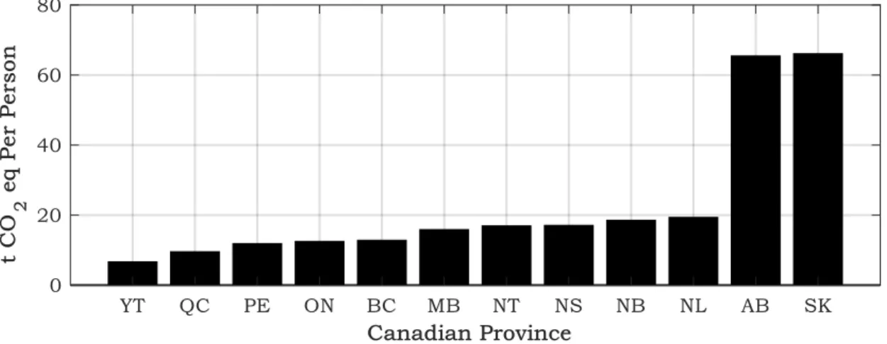
Figure 1-1: The greenhouse gas emission in Canada in 2015. ... 1

Figure 1-2: An example of the power system future scenario under high penetration of RESs. .... 2

Figure 2-1: Flowchart of the MSSSA method for obtaining the 𝑖th component. ... 25

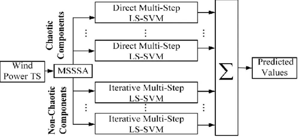
Figure 2-2: Flowchart of the proposed MSSSA-LSSVM framework. ... 31

Figure 2-3 NRMSE and computation time variation for different training dataset lengths. ... 34

Figure 2-4: The NAE error corresponding to different 6-h ahead WPP for Set 1. ... 38

Figure 2-7: NAE distribution for 6-h ahead WPP in Set 2, Oct. 2011. ... 39

Figure 2-8: NAE distribution for 6-h ahead WPP in Set 1, Feb 2012. ... 39

Figure 2-9: NAE distribution for 6-h ahead WPP in Set 3, Oct. 2016. ... 40

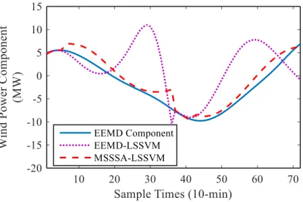
Figure 2-10: Comparing the effectiveness of MSSSA and EEMD in WPP. ... 40

Figure 2-11: 5-h ahead WPP results of MSSSA-LSSVM in Set 1 for March 2012. ... 42

Figure 2-12: 5-h ahead WPP results of MSSSA-LSSVM in Set 1 for March 2012 for 25 hours 42 Figure 3-1: The flowchart of the proposed prediction model. ... 52

Figure 3-2: Historical TCD and its ICEEMDAN components for 20 days, (a) Original time series, (b)-(j) ICEEMDAN components, (k) the residual component. ... 56

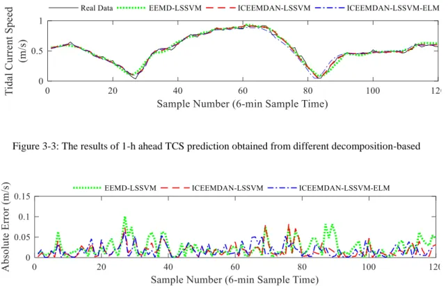
Figure 3-3: The results of 1-h ahead TCS prediction obtained from different decomposition-based prediction models. ... 57

(17)

xvi

Figure 3-5: The results of 1-h ahead TCD prediction obtained from different

decomposition-based prediction models. ... 58

Figure 4-1: The process of multilevel decomposition based on Mallat’s algorithm. ... 64

Figure 4-2: Location of wind farms in Saskatchewan, Canada 2016. ... 70

Figure 4-3: The relation between number of features and WPP. ... 72

Figure 4-4: WPP for 30-min ahead in Sunbridge wind farm. ... 74

Figure 4-5: WPP for 30-min ahead in Red Lily wind farm. ... 74

Figure 4-6: Kernel density estimation of NAE distribution of various WPP models in Sunbridge wind farm. ... 75

Figure 5-1: 𝐶𝜔, 𝜃, 𝒂 for different 𝜔. ... 88

Figure 5-2: General scheme of the proposed WPPI. ... 92

Figure 5-3: Flowchart of the proposed WPPI training procedure... 93

Figure 5-4: 10-min ahead wind power generation for AESO (Feb. 2012). ... 97

Figure 5-5: NRMSE for 10-min ahead forecasting. ... 98

Figure 5-6: Pareto front derived by the proposed WPPI for 1-step ahead (10-min ahead) prediction. ... 101

Figure 5-7: 𝑆𝑐 values for various months in training and test datasets for 𝑅𝐿 ∗= 90%. ... 102

Figure 5-8: Average 𝑃𝐼𝑁𝐴𝑊 and 𝑆𝑐 evaluation of WPPIs with 𝑅𝐿 ∗= 90% for the proposed WPPI and benchmark models for different prediction steps. ... 103

Figure 5-9: WPPIs with 𝑅𝐿 ∗= 90% constructed by the proposed WPPI in the 2nd week of Feb. 2012... 104

(18)

xvii

Figure 5-10: Convergence of convex optimization of Eq. (5-20). ... 106

Figure 5-11: Convergence of proposed WPPI for 𝑅𝐿 ∗= 90%. ... 106

Figure 6-1: Conversion of potential energy of tides to electrical energy in tidal range. ... 118

Figure 6-2: Conversion of the kinetic energy of tides to electrical energy in a tidal stream. ... 119

Figure 6-3: CDF of various probability distributions. ... 120

Figure 6-4: An illustrative example of non-uniform CDF. ... 124

Figure 6-5: The general scheme of the proposed AAQR-based NPI model. ... 126

Figure 6-6: Flowchart of the proposed AAQR-based NPI model. ... 129

Figure 6-7: 1-hour ahead prediction of the TL using the proposed AAQR-based NPI for Port Dover... 132

Figure 6-8: 1-hour ahead prediction of the TCD using the proposed AAQR-based NPI for Akutan Pass. ... 133

Figure 6-9: 1-hour ahead prediction of the TCS using the proposed AAQR-based NPI for Akutan Pass. ... 133

Figure 6-10: 1-hour ahead prediction of the TCD using the proposed AAQR-based NPI for the Bay of Fundy... 133

Figure 6-11: 1-hour ahead prediction of the TCS using the proposed AAQR-based NPI for the Bay of Fundy... 134

Figure 6-12: 𝜏 and 𝜏 for 1-hour ahead TCS prediction. ... 137

Figure 7-1: General scheme of the proposed DTLR prediction. ... 145

Figure 7-2: A schematic diagram of DTLR. ... 146

Figure 7-3: An LSTM unit ... 151

(19)

xviii

Figure 7-5: Dispersion of DTLR with respect to different feature types and Kendall 𝜏 rank

coefficient and mutual information of different features and DTLR. ... 157 Figure 7-6: Exceedance of DTLR values as the result of various prediction models; ; (a) 𝐶𝐿 ∗=

95% and (b) 𝐶𝐿 ∗= 99%. ... 161 Figure 7-7: Prediction of DTLR using the proposed model for 𝐶𝐿 ∗= 95%. ... 162 Figure C-1: Graph of convex function 𝐶(𝜔, 𝜃, 𝒂). ... 175

(20)

xix

LIST OF ABBREVIATIONS

AAQR Asymmetrically Adaptive Quantile Regression

AE Autoencoder

AESO Alberta Electric System Operator

AR Autoregressive

ARMA Autoregressive Moving Average

ARIMA Autoregressive Integrated Moving Average

CEEMD Complementary Ensemble Empirical Mode

Decomposition

CDF Cumulative Distribution Function

CL Confidence Level

CSA Coupled Simulated Annealing

CV Cross-Validation

CWC Coverage Width-based Criterion

CWT Continuous Wavelet Transform

DAE Denoising Autoencoder

DISR Double Input Symmetrical Relevance

DNN Deep Neural Network

DTLR Dynamic Thermal Line Rating

ELM Extreme Learning Machine

EEMD Ensemble Empirical Mode Decomposition

(21)

xx

EPEC Electric Power and Energy Conference

ERCOT Electric Reliability Council of Texas

FMF Fuzzy Membership Function

FORCE Fundy Ocean Research Center for Energy

FS Feature Selection

GA Genetic Algorithm

GAM Generalized Additive Model

GHGE Greenhouse Gas Emissions

GWO Gray Wolf Optimizer

HIA Hybrid Intelligent Algorithm

ICEEMDAN Improved Complete Ensemble Empirical Mode

Decomposition Adaptive Noise

IEA International Energy Agency

IESO Independent Electric System Operator

KNN 𝐾- Nearest Neighbor

LCOE Levelized Cost of Energy

LP Linear Programming

LSSVM Least Square Support Vector Machine

LSTM Long Short-Term Memory

LUBE Lower Upper Bound Estimation

MCS Monte Carlo Simulation

MI Mutual Information

(22)

xxi

MLP Mathematical-Morphology-based Local Prediction

MOD Method of Delay

MRES Marine Renewable Energy Source

MSSSA Multi-Scale Singular Spectrum Analysis

MTD Mean Trend Detector

NAE Normalized Absolute Error

NARX Nonlinear Autoregressive Exogenous

NCWC New Coverage Width-based Criterion

NMAE Normalized Mean Absolute Error

NN Neural Network

NOAA National Oceanic and Atmospheric Administration

NPI Nonparametric Prediction Interval

NRMSD Normalized Root-Mean-Squared Error Deviation

NRMSE Normalized Root-Mean-Squared Error

NWEC National Wind Energy Center

NWP Numerical Weather Prediction

OES Ocean Energy System

OHL Overhead Line

PDF Probability Distribution Function

PI Prediction Interval

PIMSE Prediction Interval Mean-Squared-Error

PINAW Prediction Interval Nominal Average Width

(23)

xxii

PSO Particle Swarm Optimization

QR Quantile Regression

QRF Quantile Regression Forest

RBFNN Radial Basis Function Neural Network

RES Renewable Energy Sources

RL Reliability Level

RMSE Root-Mean-Squared Error

RNN Recurrent Neural Network

SDAE Stacked Denoising Autoencoder

SO System Operator

SSA Singular Spectrum Analysis

STLR Static Thermal Line Rating

SUMD Sacramento Municipal Utility District

SVM Support Vector Machine

SVR Support Vector Regression

TCD Tidal Current Direction

TCS Tidal Current Speed

TEP Transmission Expansion Planning

TL Tidal Level

TS Time Series

VRES Variable Renewable Energy Source

WD Wavelet Decomposition

(24)

xxiii

WPP Wind Power Prediction

(25)

1

INTRODUCTION

General Context

Ever growing global electricity demand, fossil fuel depletion crisis, global warming concerns, and environmental pollution issues necessitate looking for alternative substitutes for electricity power generation. Figure 1-1 demonstrates the greenhouse gas emissions (GHGEs) per person in different provinces of Canada in 2015 [2, 3]. As it is apparent from this figure, Saskatchewan province is ranked first in producing greenhouse gas. Besides, according to the statistics presented in [4], in 2015, Canada was amongst the top-10 countries in GHGEs.

Since 2015, Canada, as a member of G7 [5], has aimed at cutting the GHGEs by terminating the use of fossil fuels by the end of the century [6]. The electricity sector is one of the major producers of greenhouse gases; therefore, as part of this plan, in 2016, Canada has announced phasing out the use of coal-fired electricity generation units by 2030 [7]. In support of this national transition to a cleaner electricity sector, provincial governments along with their electricity sectors have

(26)

2

planned to ambitiously increase the penetration of renewable energy sources (RESs), including hydro, wind, tides, etc.

Figure 1-2 displays an example of future power systems without coal-fired generation units. In such case, the electricity load, which is highly uncertain, should be predicted for the next day and/or next coming hours. Various load forecasting tools (i.e., [8-11]) have been developed in the literature to decrease the uncertainty of the electricity load values for the next hours. Based on the load forecasting output, the generation units which are usually far from load centers need to be economically scheduled such that the electricity demand is met. However, some degree of uncertainty in load forecast is inevitable. In this regard, operating reserve units need to be at disposal to meet the demand in the case that the demand is more than the forecasted values. On

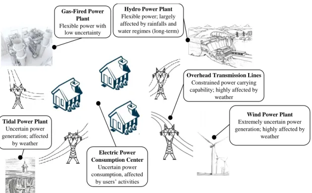
Figure 1-2: An example of the power system future scenario under high penetration of RESs.

Wind Power Plant Extremely uncertain power generation; highly affected by

weather Hydro Power Plant

Flexible power; largely affected by rainfalls and water regimes (long-term)

uncertainty) Gas-Fired Power

Plant Flexible power with

low uncertainty Electric Power Consumption Center Uncertain power consumption, affected by users’ activities

Overhead Transmission Lines Constrained power carrying capability; highly affected by

weather

Tidal Power Plant Uncertain power generation; affected

(27)

3

the other hand, in the case that the demand is lower than the scheduled power generation, some generation units need to ramp down and decrease their generation.

Changing the generation in a short period requires the high flexibility of the generation units. As shown in Figure 1-2, in the future scenario only gas-fired generation and hydropower plants are flexible, and their generation output can be dispatched in the case operating reserve or ramp down is required; while wind power generation and tidal power generation varies based on the weather [12, 13]; and therefore, they cannot be used as an operating reserve. Besides, due to the high level of uncertainty in weather and consequently wind and tidal power generation, economic scheduling of dispatchable and flexible generation units (i.e., hydro and gas-fired generation units) for the next day and/or coming hours become hardened. Accurate forecasting of the variable RESs (VRESs), e.g., wind and tidal, can substantially facilitate the power system operation problem by alleviating the VRESs uncertainty. Based on the aforementioned discussion, precise forecasting of available generation from VRESs is a key for future power systems operation.

In generation scheduling, the capability of transmission lines in carrying the available power and delivering to load center is an imperative constraint. Generally, the large-scale VRESs are far from the load centers; therefore, transmission lines are required to connect them thereto. Transmission expansion planning (TEP) requires huge investments and time. Besides, it also brings several adverse environmental impacts. Prevalently, the transmission systems are designed conservatively. In this manner, the maximum allowable power carrying capability, known as static thermal line rating (STLR), is calculated such that the transmission line’s temperature does not exceed the maximum tolerable temperature under the worst weather conditions. Unlike the conservative STLR, a dynamic thermal line rating (DTLR) estimates the transmission line’s actual ampacity under the present weather conditions [14]. The additional exploitable headroom of the transmission

(28)

4

lines can accommodate the VRESs; and thus, the need for TEP can be postponed or even omitted. As DTLR is weather dependent, the surplus transmission line ampacity varies. To effectively consider the DTLR in generation scheduling, its prediction becomes of great importance.

To recapitulate, with the increasing need for the integration of higher amount of VRESs and curtailing fossil fuel use in the electricity industry. Uncertainty in power system operation significantly increase and therefore results in unprecedented issues. Prediction of large-scale VRESs and DTLR can greatly address the power system operation problems.

Research Motivations

Wind―one of the most distributed available energy sources―is increasingly exploited for electricity generation all around the world [15]. Due to more than 40% average reduction of the levelized cost of energy (LCOE) of renewable energy generation during the last five years, nowadays, wind provides electricity competitively comparable with fossil-fuel-fired generation units in terms of overall cost [16]. Consequently, in several countries, such as Denmark, Spain, etc., wind directly participates in the market. Furthermore, several other countries, including Canada, have already considered the wind as a valuable and clean alternative, and have substantially added wind power to their electricity supply systems. As an example, in the last five years, the average growth in wind power generation capacity in Canada has an average of 23% increase per year [17]. In 2016, Canada invested $1.5 B in the wind power industry [18]. Wind energy provides approximately 5% of Canada’s total electricity and is projected to generate 20% or more of the electricity demand by 2025. Also, SaskPower set an ambitious goal of wind power penetration increment to 30% by 2030.

(29)

5

In addition to wind harnessing, marine RESs (MRESs) harvesting has recently grabbed remarkable attention across governments and power industries in the United States, Canada, Australia, France, Ireland, China, and South Korea [19]. Although the MRESs technology is still in developing stage, Ocean Energy Systems (OES) projects the potential of developing 748 GW installed MRESs by 2050 [20]. Among MRESs, tidal energy is of the main interest in Canada due to several potential sites [19]. The Bay of Fundy, located in Canada, has the highest tides in the world, it is assessed that more than 2,500 MW can be extracted from the 8,000 MW of the kinetic resource in the Bay of Fundy [21]. In this regard, Fundy Ocean Research Center for Energy (FORCE)―a not-for-profit corporation―is attracted $239.6 M funding from both public and private sectors for establishing research platform, site characterization and monitoring, and in-creasing the tidal energy capacity. In 2014, FORCE created the largest transmission capacity (64 MW) for tidal power in the world.

With the enormous investments in wind and tidal energy generation, unprecedented challenges are faced by power systems. These are mainly due to uncertainty and variability of the output generation of these VRESs, such as wind and tidal. However, employing forecasting tools and using their outputs as the input of the generation scheduling optimization problem can substantially alleviate the emerged issues [22].

With the electricity demand growth as well as the extensive VERSs exploitations, transmission lines, which are operated near their STLR constraints, may not be able to transfer the electric power due to transmission line congestions. In such a case, there are two main solutions including transmission system expansion and DTLR. The former requires vast investments and time; also, it causes several environmental concerns, while the latter can lead to an increment of the current transmission lines’ ampacity and therefore delaying the need for transmission expansion with

(30)

6

minimum costs. However, DTLR highly varies based on meteorological variables, and therefore, the maximum available transmission line capacity is uncertain.

Increasing the penetration of VRESs, including wind and tidal, surges the power systems uncertainty. On the other hand, employing the DTLR for meeting the ever-growing demand through exploiting VRESs intensifies the uncertainty in power systems. The progressively growing uncertainty can lead to several challenges in both power systems operation and planning problems. Forecasting tools can provide estimations of the available generation from VRESs and available ampacity of transmission lines. Employing the forecasting tools outcome as the input of the operation optimization problems can markedly decrease the uncertainty in VRESs and DTLR. The cost of VRESs error in forecasting manifests depending on power system operation structures. In a study conducted by Xcel Energy1_{[23], it is concluded that reduction of the normalized mean} absolute error (NMAE) by one percent would have saved over $1 million in Public Service of Colorado in 2008 [24]. Besides, the prediction model which is preferred by power producers and system operators (ISOs) are widely different from each other. For instance, some system operators like the Electric Reliability Council of Texas (ERCOT) use historical data of prediction error statistics to determine the non-spinning reserve2_{requirements. While some others like Sacramento} Municipal Utility District (SUMD) in CA, USA requires spatial and temporal variability of VRESs for energy market and dispatch decisions [16]. Therefore, the need for more accurate prediction models and different types of prediction models are the main motivations of this thesis.

1_{Xcel Energy currently manages about 7000 megawatts of installed wind power.}

2_{The non-spinning reserve, which is also known as supplemental reserve, is the ancillary generating capacity that is not currently offline and}

disconnected from the electric power grid but can be brought online within a short period of time. In an isolated electric power grid, non-spinning reserve is supplied by fast-start generators. While, in an interconnected electric system, the non-spinning reserve might be the additional power which can be imported from other electric power grids.

(31)

7

Based on the forecast horizon, prediction models can be categorized into four groups, comprising long-, medium-, short-, and very short-term prediction [12]. Long- and medium-term prediction models with horizons more than 6 hours ahead are employed for maintenance scheduling, reserve planning, unit commitment, etc., while short- and very short-term prediction models are vital for economic dispatch, electricity market clearing, regulation and control actions, etc. Physical models are preferred for prediction horizons longer than 6 hours ahead; however, statistical models are utilized for shorter horizons due to their low computational complexity and high accuracy. Due to the high importance of short-term prediction horizons, this work zeros in on developing a statistical prediction for short horizons.

Research Objectives and Scope

The main objective of this research is to provide proficient short-term prediction models required for optimal operation of electric power system in high penetration of large-scale VRESs, specifically wind and tidal. The objective of this Ph.D. study can be apportioned to six sub-objectives.

The first is to develop accurate deterministic prediction models which are capable of predicting the wind power and tidal energy. This deterministic prediction can be used for a range of power system problems, such as economic dispatch [25], energy storage sizing and planning [26], etc. The second is to develop wind power prediction (WPP) considering the spatiotemporal correlation among wind farms. Usually, several wind farms may be situated in a region; and therefore, the reflection of the correlation of wind farms power generation during the last samples with the target wind farm output in the next samples in the prediction model can enhance the prediction accuracy. The third is to address probabilistic prediction tools for robust [27] or interval optimization-based

(32)

8

[28] power system problems. The fourth is to develop DTLR forecasting model which facilitates efficient integration of large-scale VRESs to the electric power systems.

In line with the first sub-objective, in Chapters 0 and 3-, two deterministic prediction models are developed for wind and tidal prediction, respectively. According to the literature, wind power time series (TS) possesses nonlinearity and nonstationarity, which are the main culprits for inaccurate prediction of wind power. Signal processing approaches have been recently used to decompose the wind power TS into several less non-stationary and non-linear components which can be predicted more efficiently. Some recent studies reveal that wind power TS contains chaotic components. chaos is the property of some types of nonlinear system and results in wild and random looking patterns in TS. The existence of strong chaos in wind power TS can lead to inaccurate prediction. In Chapter 4-, the importance of considering different components with different frequency ranges (scales) in spatiotemporal wind power prediction modeling is analyzed, and a multiscale spatiotemporal prediction model is developed towards realizing the second sub-objective. To facilitate the power system operators with PI models which are of great importance for robust or interval-based power system optimization, prediction models for wind and tidal are respectively developed in Chapters 5-6- and 6 as the third sub-objective. In Chapter 7-, a DTLR probabilistic forecasting is proposed towards realizing the fourth sub-objective.

In this thesis, real-world data are used to develop and validate prediction models. The data are mainly available for the public. For wind power generation prediction, the data from AESO, Sotavento wind farm (located in Spain), and Saskatchewan wind farms, are used. While for tidal prediction due to unavailability of historical tidal power data, the influential factor to tidal power generation, including tidal level (TL), tidal current speed (TCS), and tidal current direction (TCD), are predicted. In the literature (e.g., [29, 30]), models are developed to estimate the tidal power

(33)

9

based on the mentioned factors. To develop tidal prediction models, the TL data from Port Dover (located in Ontario, Canada) and TCS and TCD data from Bay of Fundy (located in Nova Scotia, Canada) and Shark River Entrance (located in New Jersey, US) are used. Also, the DTLR model is developed based on the data related to M2 met tower in National Wind Energy Center (NWEC) [31].

Thesis Contributions

To achieve the objectives stated in Section 1-3, several contributions have been made to the related literature. A summary of these contributions is illustrated in the following. However, in each chapter of this manuscript-based thesis, these contributions are further elaborated.

The first contribution of this thesis is to develop a multi-step deterministic prediction model for wind power forecasting. This multi-step prediction model can be used for a range of power system problems, e.g., economic dispatch [32], energy storage planning and coordination [33], etc. The proposed prediction model consists of two main stages, including decomposition, and prediction. In the decomposition stage, a TS decomposition framework, based on considering the non-linearity, non-stationarity, and chaosity of the wind power TS. Prevalently, wind power TS is decomposed into several components using the decomposition tools, such as wavelet decomposition (WD), empirical mode decomposition (EMD), etc. Afterward, the decomposed components, which are less non-linear and non-stationary, are used to develop the prediction models. The existence of strong chaotic components can deteriorate the predictability of a TS. In recent literature, the presence of chaotic components in the decomposed wind power TS components are shown; however, no decomposition framework has been proposed to deal with these chaotic components, thus far. To this end, In Chapter 0 [12], I propose a decomposition

(34)

10

framework based on ensemble EMD (EEMD), chaotic TS analysis, and singular spectrum analysis (SSA). To realize the multi-step prediction, in the prediction stage, iterative prediction strategy is devised for non-chaotic components. While the chaotic components are predicted using direct prediction strategy, which prevents from accumulating the prediction error in predicting the chaotic components.

As the second contribution, a tidal energy prediction is proposed which considers the non-stationarity and non-linearity of the TCS and TCD TS. In the recent literature, it is shown that the TCS and TCD TS cannot be represented by a set of periodic components, and therefore, the TCD and TCS are non-stationary [34]. Besides, it is shown that TCS and TCD are nonlinear, and thus, linear prediction models, such as autoregressive moving average (ARMA), are not apposite for TCS and TCD prediction [34]. To address these issues, first, a decomposition approach named improved complete EEMD adaptive noise (ICEEMDAN), is proposed. ICEEMDAN is employed to decompose the TCS/ TCD TS into several less non-stationary components. The main reason behind proposing ICEEMDAN is to address the issues related to EEMD. Traditionally, to perform EEMD different realizations of the white noise are added to the original TS (i.e., TCS and TCD) [13]. However, using various realizations of the noise with the original TS can result in various extracted components for each noise associated TS; thus, the final components, obtained from EEMD, might vary for different sets of noise. Secondly, adding various noises can result in a different number of EMD components; therefore, the final averaging process for finding EEMD components becomes problematic. To further improve the prediction accuracy, a localized prediction model is developed. In the proposed prediction model, unlike the thus far TCD and TCS prediction, the prediction model is trained and developed based on the feature input vectors and their corresponding target, which are nearest

(35)

11

to the test feature input vector. To this end, K-nearest neighbor (KNN) is employed to identify the training set. Least square support vector machine (LSSVM), which has several advantages compared to the other prediction engines (e.g., neural networks, support vector machine, etc.) is employed to the TCS and TCD for the first time. To modify the prediction error, an error correction stage, consisting of an ensemble of extreme learning machines (ELMs), is developed. As the third contribution, a multiscale spatiotemporal wind power prediction model is developed. In this prediction model, the correlations of wind farms located in the vicinity of the target wind farms are considered, using wavelet decomposition and a mutual information-based feature selection (FS). In this prediction model, first, the wind power TS of different wind farms are decomposed into different frequency ranges (scales). Then, using FS, the most relevant scales of different wind farms in different time lags are considered as the input of the prediction engine. Afterward, localized prediction models are developed to predict the next value of each component, and the wind power generation in the next sample is predicted by aggregation of predicted values of all components.

As the fourth contribution, a WPP interval (WPPI) for short-term prediction is proposed to provide information about the wind power generation uncertainty. This WPPI can be employed as the input of different power system regulation tasks. Tuning the prediction engine is one of the most imperative steps in developing a WPPI. The prediction engine parameters are tuned using a cost function, which needs to be optimized. Most of the thus far proposed WPPI models are based on non-differentiable and non-convex cost functions, which make the use of heuristic optimization unescapable. However, heuristic optimizations are prone to be trapped in local solutions. Besides, with increasing the number of prediction parameters, which need to be tuned, finding the optimal prediction engine parameters by heuristic optimizations become

(36)

12

more troublesome. To this end, I propose a bi-level WPPI, in which the upper-level controls the quality of the WPPI based on the power system operator preference using few hyperparameters. While the lower-level tunes the ELM parameters via a differentiable and convex optimization using global optimization techniques.

As the fifth contribution, a tidal prediction interval (PI) for short-term prediction is put forward. This PI model is developed for TL, TCS, and TCD prediction, which are key factors in tidal power generation by means of different technologies. The proposed model is based on a bi-level optimization formulation, in which ELM prediction engine and quantile regression (QR) are employed. The quantile probabilities are asymmetrically and adaptively chosen in the upper-level optimization, which assesses the quality of the PIs. Additionally, the training process of ELM is amended by adaptively selecting ELM’s hidden neurons via upper-level optimization. The lower-level problem attains ELM’s output weighting coefficients by linear programming of QR. The heuristic optimization, consisting of gray wolf optimizer and simplex method, is designed to equip the NPI with high exploration and exploitation capabilities in the upper-level optimization.

As the sixth and the last contribution, a probabilistic DTLR is introduced for short-term power system operation problems. The proposed DTLR PI model benefits from new predictors which can provide valuable information about DTLR by representing the highly nonlinear and complex relation of DTLR values with meteorological variables. Besides, in the DTLR PI, for the first time, a deep neural network (DNN) is adapted as the prediction engine. Stacked denoising autoencoder (SDAE) is employed for feature extraction and dimension reduction. The DNN is composed of recurrent neural networks (RNNs) which are more suitable in TS

(37)

13

forecasting. A novel cost function, defined to facilitate the training of the prediction model for probabilistic forecasting, is another valuable feature of this work.

Thesis Organizations

The rest of this manuscript-based thesis is as follows.

Chapter 0 is titled “A novel multi-step short-term wind power prediction framework based on chaotic time series analysis and singular spectrum analysis.” In this Chapter, the proposed multi-step deterministic wind power prediction, which is published in IEEE Transactions on Power Systems, is described. Mr. G. C. D. Price is a co-author of this paper, and he provided me with invaluable technical comments. Also, he helped me to evaluate the proposed model using the Centennial wind power generation. I developed and implemented the model, performed the simulation, and analyzed the results, along with the paper write-up

Chapter 3- is titled “An advanced multistage multi-step tidal current speed and direction prediction model.” This chapter presents the proposed deterministic prediction for TCS and TCD, which has been published as an article in Proceedings of the Electric Power and Energy Conference (EPEC), Saskatoon, Saskatchewan, CA, October 2017. Mr. Khorramdel and Mr. Zare assisted me in preparing the presentation and programming the forecasting model in MATLAB software. I developed and implemented the model, performed the simulation, and analyzed the results, along with the paper write-up

Chapter 4- titled “A spatiotemporal wind power prediction based on wavelet decomposition, feature selection, and localized prediction.” This chapter demonstrates the multiscale spatiotemporal wind power prediction modeling, which has been published as an article in Proceedings of the EPEC, Saskatoon, Saskatchewan, CA, October 2017. Ms. Y. Chen, Mr. B.

(38)

14

Khorramdel, and Mr. L. P. Mao assisted me in developing the model in MATLAB and preparing the presentation. I developed and implemented the model, performed the simulation, and analyzed the results, along with the paper write-up.

Chapter 5- titled “Very short-term wind power prediction interval framework via bi-level optimization and novel convex cost function.” This chapter describes the proposed wind power PI, which has been submitted to IEEE Transactions on Power systems for the third round of revision.

Dr. Mazhari as the co-author provided invaluable comments and suggestions during the development of the model. I developed and implemented the model, performed the simulation, and analyzed the results, along with the paper write-up.

Chapter 6- is titled “Tidal current and level uncertainty prediction via adaptive linear programming.” This chapter demonstrates the proposed tidal PI, which has been published in IEEE Transactions on Sustainable Energy. Dr. Mazhari as the co-author provided invaluable comments and suggestions during the development of the model. I developed and implemented the model, performed the simulation, and analyzed the results, along with the paper write-up.

Chapter 7- is titled “A secure deep probabilistic dynamic thermal line rating prediction.” This chapter demonstrates the proposed DTLR probabilistic prediction, which is going to be submitted to IEEE Transactions on Power Systems. Dr. Mazhari as the co-author provided invaluable comments and suggestions during the development of the model. Dr. S. B. Ko provided priceless comments on presentation of the proposed model. I developed and implemented the model, performed the simulation, and analyzed the results, along with the paper write-up. The conclusions of this thesis are provided in Chapter 8-.

(39)

15

A NOVEL MULTI-STEP SHORT-TERM WIND POWER

PREDICTION FRAMEWORK BASED ON CHAOTIC TIME SERIES

ANALYSIS AND SINGULAR SPECTRUM ANALYSIS

3

Decomposition methods are widely applied as a prestage of wind power prediction (WPP) to reduce the prediction errors caused by the nonstationarity and nonlinearity of wind power time series (TS); however, they cannot address the issues posed by the chaotic behavior of wind power TS. This paper, therefore, proposes a novel decomposition approach to take the chaotic nature of wind power TS into account and to improve WPP accuracy. In this decomposition approach, as a primary step, the wind power TS is separated into several components with different time-frequency characteristics (scales) by means of ensemble empirical mode decomposition. Chaotic TS analysis is then applied to determine which components are chaotic, and then singular spectrum analysis (SSA) is applied thereto. This multi-scale SSA (MSSSA) can maintain the general trend of chaotic components, which become smoother by eliminating extremely rapid changes with low amplitudes, and thus several steps ahead WPP with higher accuracy can be realized. Following the proposed decomposition, a novel short-term WPP method comprised of localized direct and iterative prediction is proposed to perform multi-step prediction for the chaotic and nonchaotic components of MSSSA, respectively. The proposed framework is finally validated using historical data related to overall wind power generation for Alberta (Canada), the Sotavento wind farm (Spain), and Centennial wind farm in Saskatchewan (Canada).

prediction framework based on chaotic time series analysis and singular spectrum analysis,” IEEE Trans. Power Syst., vol. 33, no. 1, pp. 590-601, Jan. 2018.

(40)

16

Introduction

Duo to high intermittency and non-dispatchability, large-scale wind power integration creates new challenges in power system operation, but these can be significantly alleviated by short-term wind power prediction (WPP) [35]. Existing WPP methods are mainly based on three types of prediction models: physical models [36], statistical models [37, 38], and hybrid models (combining aspects of physical and statistical models) [39, 40]. Physical models are based on detailed physical descriptions of terrain and wind farm layout as well as simulation results obtained from numerical weather prediction (NWP), while statistical models only require time series (TS) of historical data such as wind speed and wind power [38]. Due to the high computational cost of NWP, physical models based on NWP are not preferred for short-term WPP (≤ 6-h ahead) [35]. Because hybrid models also require results of NWP, their application to short-term WPP is also limited. In contrast, statistical WPP models have lower cost and complexity and therefore can be used for shorter-term WPP [37, 38].

Generally, statistical WPP can be classified into two types: indirect and direct prediction. In indirect prediction, wind speed values are first predicted and then mapped into wind power by a parametric or non-parametric wind power curve (e.g., [38, 39, 41, 42]). An accurate wind power curve requires data for several environmental and meteorological variables [43], but such variables have not been considered in indirect prediction [44]. Consequently, the indirect prediction has limited accuracy. In direct prediction, wind power is directly predicted from historical data (e.g., [37, 45, 46]), resulting in greater accuracy [44, 47].

Most recent direct statistical WPP methods [37, 46, 48-50] decompose the TS into several components with different characteristics [51] as a pre-stage of prediction; this remedies the

(41)

17

inaccuracy originating from the non-linearity and non-stationarity of the original TS. In [46], a morphological-based decomposition approach for separating wind power TS into a mean trend component and a stochastic component is proposed. In [37, 49], the effectiveness of the wavelet transform (WT) decomposition method is assessed. Recently, a few studies in WPP have employed empirical mode decomposition (EMD) variants [48, 50]. Generally, WT decomposition requires some prior knowledge and assumptions about the TS to find an appropriate mother wavelet, while EMD is a data-driven heuristic method that does not need initial assumptions about TS shape prior to decomposition [52]. A comprehensive comparison of the performance of EMD vs. WT variants shows the superiority of the former [50]. Ensemble EMD (EEMD) has the best performance in terms of improvement in WPP accuracy compared to other EMD variants and WT [50]. Additionally, the low computational complexity of EEMD has been theoretically demonstrated [53], confirming its suitability in terms of a low computational burden for short-term WPP. Although decomposition methods can deal with the non-linearity of the components to a large extent, the components obtained from wind power TS can still be of a chaotic nature, which can lead to prediction errors [54]. In a chaotic component, some subcomponents highly fluctuate in unpredictable patterns with low amplitudes [55, 56]. Singular spectrum analysis (SSA) can remove highly fluctuating and low amplitude variations from the chaotic TS, and therefore significantly improve the accuracy of the prediction [56]; however, this has not yet been applied to WPP as a supplementary tool for decomposition processes to handle the chaotic behavior of wind power TS. After decomposition, various prediction methods can be used for WPP. Machine learning tools including neural networks (NNs) and support vector machines (SVMs) have recently been employed for this purpose due to their efficiency in predicting non-linear TS (e.g., [46, 57]). In [57], a comparative study of the conventional statistical approach known as autoregressive

(42)

18

integrated moving average (ARIMA) and NNs shows the superiority of the latter approach. Recently, a modified SVM, known as least squares-SVM (LSSVM), was successfully employed in WPP [46, 58]. LSSVM demonstrates better performance than SVM and NNs in terms of computational burden, simplicity, and the probability of convergence to global minima [58].

For all of the methods mentioned above, the prediction model should first be trained. Global [58] and localized [46] training are two possible training procedures that can be utilized. Localized prediction with an on-line training process, which makes use of historical data points that are very similar to the most recent data points, has superior performance in terms of prediction accuracy compared to global fitting approaches [46, 59]. Localized prediction focuses only on predicting the upcoming output from the current data point; hence, the model should be kept updated by historical data points with the smallest Euclidean distance to the most recent data points.

According to prediction output, statistical WPP models proposed in the literature can be categorized into probabilistic prediction [60], prediction interval [45], and deterministic prediction [46-52]. Probabilistic prediction and prediction interval are the extension of deterministic WPP to model the uncertainty in prediction [61]. Having information about WPP uncertainty is very useful. However, system operators need probabilistic or interval WPP results accompanied by deterministic WPP to make an optimal decision [62]. Deterministic WPP can be interpreted as the most likely wind power [27]. The application of deterministic WPP has been reported for short-term power system security [35], various unit commitment strategies [63], energy storage sizing [26], etc. In addition, a deeper understanding of the chaotic behavior of TS, such as wind power, can significantly reduce the prediction uncertainty and make the predicted value closer to the actual value [59]. For the aforementioned reasons, this paper aims at developing deterministic WPP

(43)

19

framework and improving prediction accuracy by proposing a deterministic chaotic time series analysis-based WPP.

Multi-step WPP is crucial for multi-step optimization problems such as unit commitment [64]. Several machine learning algorithms can be used in multi-step prediction; however, only a limited number of studies have been carried out for short-term multi-step WPP [46]. Multi-step prediction can be divided into direct prediction and iterative prediction. In the latter approach, the predicted values from previous steps are used to predict the next step; in the former approach, the predicted values at different steps are only calculated based on historical data. Iterative prediction is appropriate for predicting multi-step non-chaotic TS while multi-step direct prediction is suitable for chaotic TS [59, 65]. Indeed, iterative prediction can lead to significant accumulative error in predicting chaotic components [59]; however, hitherto no WPP has employed direct and iterative prediction methods to predict chaotic and non-chaotic components, respectively.

From the above discussion, the main purpose of this paper is to consider both the chaotic and non-chaotic natures of wind power TS. Considering the distinguishing characteristics of chaotic and non-chaotic components in both decomposition and prediction stages can result in a significant increase in WPP accuracy. In this regard, a novel decomposition stage based on the proposed multi-scale singular spectrum analysis (MSSSA) is developed. The MSSSA is used to decompose the wind power TS. Utilizing MSSSA alleviates the issues related to wild patterns in wind power TS. MSSSA consists of three main building blocks: EEMD, chaotic TS analysis, and SSA. EEMD is first applied to wind power TS, resulting in decomposition of TS into several components (scales). Then, by employing chaotic TS analysis, chaotic components (scales) are detected. To increase the predictability of the chaotic components, the wildest and most unpredictable subcomponents in each scale (component) are recognized based on SSA. Thereafter, the chaotic

(44)

20

components are processed to make them smoother and more predictable. Hence, this MSSSA framework is different from the decomposition-based WPP models presented thus far. After the decomposition stage, a localized LSSVM-based framework is employed and a multi-step short-term WPP method is proposed that comprises localized direct and iterative prediction of chaotic and non-chaotic components, respectively. Using direct multi-step prediction helps to avoid the accumulated error in the prediction of chaotic components, while iterative multi-step increases the accuracy of the prediction for non-chaotic components. The proposed framework that comprises MSSSA and LSSVM is herein named MSSSA-LSSVM.

To see the effectiveness of the proposed WPP in the prediction of aggregated wind power generation, as well prediction of wind farm generation, data from Alberta Electric System Operator (AESO), in Canada, Sotavento wind farm located in Spain, and Centennial wind farm, in Saskatchewan, Canada, are reported. Several well-established WPP models have been employed to confirm the superiority of the proposed MSSSA-LSSVM.

The remainder of this paper is organized as follows. Section 2-2 presents the proposed decomposition method. Section 2-3 introduces the proposed multi-step WPP. Data, evaluation indices, and simulation results of the proposed MSSSA-LSSVM framework are discussed in Section 2-4. Section 2-5 concludes the paper.

Decomposition Method

This section first provides a brief overview of EEMD, chaotic TS analysis, and SSA, and then introduces the proposed decomposition method in detail.

(45)

21

EEMD

EEMD is obtained from an ensemble of NE (number of generated trials from combinations of the original TS and white noises) EMDs. Hereafter, we assume 𝑥(𝑛𝑇_𝑆) is the TS of wind power,

n is the sample number with 𝑇_𝑆 sampling time, and N is the total number of available samples. Decomposing the wind power TS with EEMD can be summarized according to the following steps. A detailed explication can be found in [66].

1) Add white noise (𝑤_𝑗(𝑛𝑇𝑆), 𝑗 = 1, … , 𝑁𝐸) to the original TS (𝑥(𝑛𝑇𝑆)) to construct 𝑁𝐸 trials

of TS (𝑥(𝑛𝑇𝑆)) as follows:

𝑥_𝑗(𝑛𝑇_𝑆) = 𝑥(𝑛𝑇_𝑆) + 𝑤_𝑗(𝑛𝑇_𝑆) (2-1)

then perform Steps 2-6 for every trial (𝑗) to find corresponding EMD components. 2) Find the local maxima and local minima of 𝑥𝑗(𝑛𝑇𝑆).

3) Interpolate the identified local maxima and minima points to find the upper envelope (

𝑈𝐸_𝑗(𝑛𝑇𝑆)) and lower envelope (𝐿𝐸𝑗(𝑛𝑇𝑆)) of 𝑥𝑗(𝑛𝑇𝑆) respectively.

4) Calculate the difference between 𝑥𝑗(𝑛𝑇𝑆) and the mean of 𝑈𝐸𝑗(𝑛𝑇𝑆) and 𝐿𝐸𝑗(𝑛𝑇𝑆) as

follows:

𝑚𝑗(𝑛𝑇𝑆) = 𝑥𝑗(𝑛𝑇𝑆) −

𝑈𝐸_𝑗(𝑛𝑇𝑆) + 𝐿𝐸𝑗(𝑛𝑇𝑆)

2 (2-2)

5) Repeat Steps 2-4 with 𝑚_𝑗(𝑛𝑇_𝑆) instead of 𝑥_𝑗(𝑛𝑇_𝑆), until 𝑈𝐸𝑗(𝑛𝑇𝑆)+𝐿𝐸𝑗(𝑛𝑇𝑆)

2 ≤ 𝜀 (where 𝜀 is

the acceptable error and should be close to zero), then keep 𝑐_𝑗1(𝑛𝑇_𝑆) = 𝑚_𝑗(𝑛𝑇_𝑆) as the first EMD component of𝑥𝑗(𝑛𝑇𝑆). At this stage, the residue 𝑟𝑗1(𝑛𝑇𝑆) = 𝑥𝑗(𝑛𝑇𝑆) − 𝑐𝑗1(𝑛𝑇𝑆) is then

(46)

22

6) Given 𝑐_𝑗𝑖(𝑛𝑇𝑆) and 𝑟𝑗𝑖−1, for 𝑖 > 1 then 𝑐𝑗𝑖+1(𝑛𝑇𝑆) can be calculated by setting 𝑟𝑗𝑖(𝑛𝑇𝑆) =

𝑟_𝑗𝑖−1(𝑛𝑇𝑆) − 𝑐𝑗𝑖(𝑛𝑇𝑆) and repeating Steps 2-5 with 𝑥𝑗(𝑛𝑇𝑆) replaced by 𝑟𝑗𝑖(𝑛𝑇𝑆) .

Theoretically, the above iteration should continue until the residue becomes monotonic; however, different stoppage criteria are required to find the appropriate number of necessary components [51, 66]. In this paper, the number of required components (𝑀) is selected based on a tradeoff between computational burden and monotonicity. Based on this process,

𝑥𝑗(𝑛𝑇𝑆) can be decomposed into different EMD components as follows:

𝑥_𝑗(𝑛𝑇𝑆) = ∑ 𝑐𝑗𝑖(𝑛𝑇𝑆) + 𝑟𝑗𝑀(𝑛𝑇𝑆) 𝑀

𝑖=1

(2-3) 7) Calculate the components of EEMD (𝑐𝑖(𝑛𝑇𝑆)) by averag-ing the respective components

(𝑐𝑖(𝑛𝑇𝑆)) of all trials.

Finally, 𝑥(𝑛𝑇_𝑆) can be reconstructed as follows:

𝑥(𝑛𝑇_𝑆) = ∑ 𝑐𝑖_(𝑛𝑇

𝑆) + 𝑟𝑀(𝑛𝑇𝑆) 𝑀

𝑖=1

(2-4) where 𝑟𝑀(𝑛𝑇𝑆) is the residue and calculated by averaging 𝑟𝑗𝑀(𝑛𝑇𝑆), 𝑗 = 1, … , 𝑁𝐸. Notably,

the amplitude of the residue is very small and hence is negligible in WPP.

Chaotic TS Analysis

Chaotic TS has wild and non-periodic behaviors [59] and its chaosity can be determined by its corresponding maximal Lyapunov exponent (MLE) (Appendix A). To find the MLE, the TS must first be embedded in a multidimensional space to form the trajectory matrix. This can be done with the method of delays (MOD) [67]. In such an embedding, each point in multidimensional space is

(47)

23

a vector whose components are the delayed version of the TS. In this multidimensional space, Lyapunov exponents determine the exponential convergence or divergence of nearby points, and MLE is the largest Lyapunov exponent that shows the largest convergence or divergence. If the sign of MLE is positive, then the TS is recognized as a chaotic TS; otherwise, it is non-chaotic. A detailed discussion of the MLE, as well as the program for calculating it, is available in [67].

SSA

A TS is comprised of several intrinsic components with different time-frequency characteristics [55]. SSA is a non-parametric spectral extraction method that can be used to separate the general trend, fluctuations, and noise components in a TS. First, to find components of the TS by means of SSA, the TS is mapped into a multidimensional space by the construction of the trajectory matrix. Then, eigenvalues and corresponding eigenvectors of the trajectory matrix are calculated by means of singular value decomposition. Using eigenvectors, the components in the trajectory matrix corresponding to every eigenvalue can be extracted. Next, in a grouping stage, the components which share some similarity are grouped together. In the last step, using diagonal averaging [55], the grouped components should be mapped from reconstructed multidimensional space to form a TS.

The smallest eigenvalues in SSA correspond to components with the smallest amplitudes, highest fluctuations, or noise, which are called non-informative (as they do not provide useful information and distort the main trend of the TS); the largest eigenvalues (dominant eigenvalues) are related to the highest amplitudes and smallest variations (i.e., the general trend of the TS) [55].

Using the advantages of SSA, the components obtained from SSA can be grouped into informative and non-informative groups. In other words, SSA can reconstruct the TS with

(48)

24

informative components (large eigenvalues), thereby increasing the prediction accuracy.Further information on SSA can be found in [56].

Proposed MSSSA Decomposition Method

Figure 2-1 shows the flowchart of the proposed MSSSA decomposition method for obtaining its

ith component. The detailed procedure of the proposed method is also provided as follows: 1) Apply EEMD to find components related to wind power TS by following the procedure

described in Section 2-2-1.

2) Identify the chaotic and non-chaotic components based on chaotic TS analysis as explained in Section 2-2-2.

3) Carry out SSA as described in Section 2-2-3 for any chaotic components, while non-chaotic components remain unchanged. To perform SSA for a chaotic component, the corresponding trajectory matrix by means of MOD is constructed. If 𝑐𝑖(𝑛𝑇_𝑆) in Eq. ((2-4) is a chaotic component, the corresponding trajectory matrix can be defined as

𝑪𝑖 _{= [𝐶}

1𝑖 𝐶2𝑖 ⋯ 𝐶𝑙𝑖 ⋯ 𝐶𝑚𝑖 ]𝑑×𝑚𝑇 (2-5)

where 𝑑 is the number of lags (or embedding dimension) and its appropriate value [54] can be found based on Cao’s method [68]. C