On the external validity of experimental
inflation forecasts:
A comparison with five categories
of field expectations
Camille Cornand
Paul Hubert
EDITORIAL BOARD
Chair: Xavier Ragot (Sciences Po, OFCE)
Members: Jérôme Creel (Sciences Po, OFCE), Eric Heyer (Sciences Po, OFCE), Lionel Nesta (Université Nice Sophia Antipolis), Xavier Timbeau (Sciences Po, OFCE)
CONTACT US
OFCE
10 place de Catalogne | 75014 Paris | France Tél. +33 1 44 18 54 87
www.ofce.fr
WORKING PAPER CITATION
This Working Paper:
Camille Cornand et Paul Hubert
On the external validity of experimental inflation forecasts: A comparison with five categories of field expectations
Sciences Po OFCE Working Paper, n° 03
Downloaded from URL : www.ofce.sciences-po.fr/pdf/dtravail/OFCEWPWP2019-03.pdf DOI - ISSN
ABOUT THE AUTHOR
Camille Cornand Univ Lyon, CNRS, GATE Email Address: [email protected] Paul Hubert OFCE, Sciences Po, Paris* Email Address: [email protected]
ABSTRACT
Establishing the external validity of laboratory experiments in terms of inflation forecasts is crucial for policy initiatives to be valid outside the laboratory. Our contribution is to document whether different measures of inflation expectations based on various categories of agents (participants to experiments, households, industry forecasters, professional forecasters, financial market participants and central bankers) share common patterns by analyzing: the forecasting performances of these different categories of data; the information rigidities to which they are subject; the determination of expectations. Overall, the different categories of forecasts exhibit common features: forecast errors are comparably large and autocorrelated, forecast errors and forecast revisions are predictable from past information, which suggests the presence of information frictions. Finally, the standard lagged inflation determinant of inflation expectations is robust to the data sets. There is nevertheless some heterogeneity among the six different sets. If experimental forecasts are relatively comparable to survey and financial market data, central bank forecasts seem to be superior.
KEY WORDS
Inflation expectations, experimental forecasts, survey forecasts, market-based forecasts, central bank forecasts
JEL
E3, E5, E7
* We would like to thank Klaus Adam, Cars Hommes, Domenico Massaro, Damjan Pfajfar, Matthias Weber and Blaz Žakelj for sharing their experimental data. We also thank Christophe Blot and Pauline Gandré for detailed feedbacks, and participants to the 2018 BEAM-ABEE workshop, in particular John Duffy, Cars Hommes, Simas Kucinskas, Tomasz Makarewicz, and Baptiste Massenot for valuable comments.
1.
Introduction
Understanding the formation of economic agents’ inflation expectations is crucial for the conduct of monetary policy. Recently a growing macro-experimental literature has focused on inflation expectations formation in the laboratory. Laboratory experiments – in particular Learning-to-Forecast Experiments (LtFE)1 (see Hommes (2011) for a survey) – are used to validate expectations hypotheses
and learning models. These experiments may also serve as an important tool for central bankers, by providing a test-bed for competing policy actions or monetary policy rules (Cornand and Heinemann, 2014, 2018). The external validity of expectations is critical for policy initiatives to be valid outside the laboratory (Duffy, 2008).2
The question of how agents form inflation expectations is generally studied owing to survey data on expectations of future inflation. Survey data present the advantages (over experimental data) to provide ‘natural’ expectations, that are, in principle, more representatively sampled and should be subject to more external validity. However, they present the inconvenience to pay a fixed reward, implying that there is no incentive for economic agents to provide an answer that is as accurate as possible.3 Extracting expectations from financial instruments (such as swaps) provides a response to
the lack of incentives. But they are no direct observations of expectations and their extrapolation may interfere with biases or other uncontrolled elements (yielding a problem of testing joint hypotheses). While survey measures are not directly linked to financial decisions, market-based measures incorporate liquidity or risk premia. In contrast, laboratory experiments provide data on expectations that respond to incentives. They also offer data, whose generating process is perfectly known by the experimenter and provide the experimenter with a large number of independent observations.4
Overall, all inflation expectations data (experimental data, market-based data, survey data and central bank data) have some relative advantages and drawbacks, and provide an overview of how economic agents form inflation expectations, how successful they are in forming these forecasts, how much these expectations are rational (or depart from rationality), to what extent they are subject to information rigidities, and what variables enter their determination.
The debate on the external validity of experimental inflation forecasts echoes the issue – pointed by Carroll (2003) among others – of the heterogeneity between the inflation expectations of various categories of agents – professional forecasters, industrial forecasters, central bankers, households, financial market participants – and how each of these groups form expectations. While the literature has provided some comparisons of survey measures of inflation expectations (see e.g. Thomas (1999)
1 In LtFE, participants in the experiment play the role of professional forecasters. Their task is to provide their expectation
about an economic variable (for example the market price or in the case we are interested in, inflation). Their payoffs depend negatively on their forecast error. The expectations that are formed by subjects in the laboratory are aggregated (either by mean or median) and this summary statistic is introduced into the theoretical model as the aggregate expectation of agents. Most recent experiments on DSGE models use variants of the standard three equations: IS-curve, Phillips curve, and policy rule. This model is directly implemented via a computer program, except the expectations that are determined by participants to the experiment. The computer program derives the current values of variables conditional on the model parameters, which yields, period after period, time series of the main variables.
2 External validity is particularly important for macro-experimentalists as they necessarily recourse to small-scale laboratory
evidence. A complementary line of research consists in testing the robustness of macro-experiments when considering large group size (100 participants) instead of the standard 6 to 10 participants’ group size. See Hommes et al. (2018).
3 In fact, some surveys conducted toward professionals introduce incentives to respond as accurately as possible. For
example, the publisher of Blue Chip Economic Indicators organizes an annual dinner during which the most accurate forecaster of the previous year is honored and identified in later issues of the newsletter. Something similar is organized by the central bank of Brazil for professional inflation forecasts.
for such a study on US data), a comparison across types of measures (survey, market-based, central bank, and also experimental) based on various categories of agents (including household, industry, professional forecasters, financial market participants, central bankers, and also participants to laboratory experiments) has not been examined yet. Our contribution is therefore to document whether different types of measures share common patterns by analyzing:
The forecasting performances of these different types of data (following Diebold and Mariano (1995), Romer and Romer (2000), Ang, Bekaert and Wei (2007));
The information frictions to which they are subject (following Andolfatto, Hendry and Moran (2007), Coibion and Gorodnichenko (2012, 2015), Andrade and Le Bihan (2013));
The formation process of expectations and the variables entering this process (following Mankiw and Reis (2002), Sims (2003), Lanne, Luoma and Luoto (2009), Pfajfar and Santoro (2010), Fendel, Lis and Rülke (2011), Dräger, Lamla and Pfajfar (2016)).
While these analyses (forecasting performance, information rigidities, determination of expectation formation) have been conducted separately and have excluded experimental data, this paper precisely aims at conducting these analyses in parallel in order to have a large set of characteristic comparisons and at enlarging the data sets by including experimental inflation expectations. These comparisons intend to determine whether the various sets of inflation expectations exhibit heterogeneous or common patterns and thus to examine the external validity of experimental inflation forecasts. We therefore use standard measures of forecast characteristics, information rigidity and expectation formation determination that we apply to each of our different sets of expectations:
Assess the characteristics of forecast errors
To this aim, we analyze for each of our different samples (experimental, survey, financial market and central bank data) whether forecast errors are significant in order to evaluate whether economic agents (participants to laboratory experiments, households, industry, professional forecasters, financial market participants, central bank staffs and policymakers) make systematic mistakes, i.e. form biased inflation expectations. We also measure the magnitude of absolute forecast errors in order to establish the forecasting quality of our different samples.
Assess the informational frictions affecting forecast errors
In order to evaluate whether and to what extent expectations are formed on the basis of the information available to our different categories of economic agents, we study for each of our different samples whether forecast errors are autocorrelated, correlated to forecast revisions and whether forecast revisions depend on past forecast revisions. We compare how our different categories of agents take into account available information.
Evaluate the usual determinants of inflation forecasts
We study how lagged inflation and output gap affect inflation forecasts in order to evaluate whether the usual determinants of inflation are used by the different considered categories of agents.
While establishing the external validity of laboratory experiments in terms of inflation expectation represents a key step for the development of macro-experiments, especially those dealing with
monetary policy issues, to our knowledge, there is no available study relying on a sample of experimental data on inflation expectation confronting it with field data.5 The aim is also to inform the
policymaker about the informativeness of the different types of data.
In spite of the considerable heterogeneity among our six different categories of data, we find that the different datasets exhibit various common features: forecast errors are comparably large; autocorrelations of forecast errors are positive and significant, forecast errors and forecast revisions are very often predictable, which suggests the presence of information frictions; the standard lagged inflation determinant of inflation expectations is robust to the data sets. There is nevertheless some heterogeneity among the six different sets. If experimental forecasts are relatively comparable to survey and financial market data, central bank’s forecasts seem superior, as they do not exhibit systematic bias, are less autocorrelated, and hardly predictable. Excluding central bank forecasts, we conclude that experimental data are reasonably comparable to other data sets in the sense that forecast errors exhibit the same kind of bias (except for industry forecasts) and lagged forecast revisions enter significantly and usually negatively in forecast revisions.
The paper is structured as follows. Section 2 presents the data. Section 3 describes the empirical results. Section 4 concludes the paper.
2.
Data
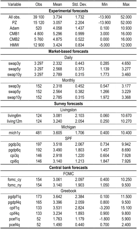
We collect inflation expectation forecast data for four different types of measures of inflation expectations (experimental data, survey data, financial market data, and central bank data) corresponding to six categories of agents (participants to experiments, households, industry, professional forecasters, financial market participants, central bank’s staffs and policymakers). We also collect macroeconomic data. Descriptive statistics of the different series are provided in Table A in the Appendix.
We acknowledge the heterogeneity of the different datasets with respect to their forecasting horizons, their frequency, and the sample period considered. Regarding the horizon and frequency, while they may be different from one set to the other, it is worth stressing that for all categories of agents, they correspond to the relevant horizon and frequency for their respective usual economic decisions, while the forecasting horizon and frequency in experimental forecasts are abstract. Regarding the sample period for field data, we focus our empirical analysis on a relatively recent sample period, from 1987 to 2017, for comparability purposes between types of agents as well as macroeconomic and structural environments. Two exceptions are inflation swaps that start in 2004 and Greenbook forecasts that end in 2012.6
5 Some recent papers have focused on establishing the external validity of experiments on expectation formation in a different
manner. In particular, Armantier et al. (2015) present a study in which they compare survey data on inflation expectations reported by consumers to the behavior of the same subjects in a financially incentivized investment experiment. They show that the survey is informative: stated beliefs in the survey and experimental decisions are highly correlated and conform to theoretical predictions. Armantier et al. (2017) somehow mix experimental and survey methods in order to investigate how consumers’ inflation expectations respond to new information. They randomly provide a subset of agents with factual information (i.e. either past-year average food price inflation or the average forecast of next-year overall inflation in the Survey of Professional Forecasters). They are thus able to identify causal effects of new information on agents’ expectations. Our methodology and aim are different: we investigate whether experimental data share the same pattern as field data.
6 At least for experimental, survey and central bank data, there is also some heterogeneity inside samples as the way data
are collected (type of survey or type of design and model behind experiments) and the category of economic agents can vary. A priori, there is no reason for one sample to be more heterogeneous than another.
2.1. Data from laboratory experiments (from various published research papers)
We collect a sample of macro-experimental data on inflation expectations formation from published papers. In these experiments, participants are mainly students.
The first paper is that of Pfajfar and Žakelj (2018), which presents a LtFE (conducted at the University Pompeu Fabra in Spain and the University of Tilburg in the Netherlands) based on a simple version of forward-looking sticky price New Keynesien model. They ask subjects to form inflation expectations (more precisely, a prediction of the t+1 period inflation and the 95% confidence interval of their inflation prediction), but no output gap expectation (instead the computer program feeds the model with naïve output gap expectations). The economy is subject to two types of shocks: a government spending shock or taste shock and a cost-push shock. They consider four different treatments, corresponding to four different policy rules: inflation forecast targeting, with three different degrees of monetary policy aggressiveness; and contemporaneous inflation targeting, with an intermediate degree of monetary policy aggressiveness (the target is 3%).7 Subjects observe the history of
macroeconomic variables: at each period t, participants observe inflation, the output gap and the interest rate up to period t-1.8 There are 70 periods, each period corresponds to a quarter. The number
of observations amounts to 24 independent groups.
The second one is Adam (2007). The experiment took place at the University of Salerno in Italy and at the Goethe University of Frankfurt in Germany. Hefocuses on a monopolistic competition framework. Participants in the experiment play the role of firms that set prices one period in advance and have to form inflation forecasts 2 periods ahead (even though prices are sticky for a single period only). In any period t, subjects observe history of output and inflation up to period t-1, and are asked to forecast inflation for periods t and t+1.9 The economy is subject to shocks (mean zero white noise shock with
small bounded support). There are 6 independent groups.10
The third one is Cornand and M’baye (2018), who focus on a design that is very close to that of Pfajfar and Žakelj (2018). Their experiment relies on the same model, but the considered parameter values are slightly different. Cornand and M’baye asked subjects to state inflation expectations, but not output expectations, although the macro-model behind the experiment requires both. As in Pfajfar and Zakelj (2014), Cornand and M’baye assumed that firms naively expect the same level of aggregate output as realized in the last period. Cornand and M’baye (2018) study the role of central bank’s inflation target communication by comparing treatments in which the central bank explicitly announces its inflation target to treatments in which the central bank does not announce the target. They consider four treatments differing by the type of inflation targeting procedure.11 An important
7 Their aim is to study which targeting rule best stabilizes the economy. They find that a higher degree of monetary policy
aggressiveness reduces the variability of inflation, but may lead to cycles and that contemporaneous inflation targeting outperforms inflation forecast targeting for a same degree of monetary policy aggressiveness.
8 Regarding initial values, before the experiment starts, subjects observe inflation, the output gap, and the interest rate from
periods -9 to 0, which are generated under the assumption of rational expectations.
9 The experiment is in between a LtFE and a LtOE: there is an additional optimization task, but subjects neither know the
steady state nor any feature of the underlying economy. Note that only average forecasts per group (and not individual ones) were available.
10 Two treatments were considered: four sessions were subject to the high-elasticity treatment, two sessions to the low
elasticity treatment.
11 More precisely, these treatments are: (1) Implicit strict inflation target, in which the central bank does not announce its
inflation target to the public and its sole objective is to stabilize inflation; (2) Explicit strict inflation target, in which the central bank explicitly communicates its 5% inflation target and its sole objective is to stabilize inflation; (3) Implicit flexible inflation target, in which the central bank does not announce its target for inflation to the public and the central bank both has an
point is that agents are given information about the target, so there may be a forward-looking component to their expectation, in contrast to Adam or Pfajfar and Žakelj. For each treatment, they have 4 sessions with 6 subjects each. Each session lasted for 50 periods.
The fourth paper is Cornand and M’baye (2016), who are similar to Cornand and M’baye (2018) in terms of design. They consider 4 different treatments differing with respect to whether the central bank implemented a band or point target and differing also by the size of shocks.12 They had 4 sessions
with 6 subjects for each treatment. Sessions lasted for 60 periods. Both experiments by Cornand and M’baye took place at the GATE-LAB of the University of Lyon in France.
The fifth paper is Hommes et al. (2017), which presents a LtFE (conducted at the CREED lab at the University of Amsterdam in the Netherlands) based again on a simple standard version of the New Keynesien model, with similar characteristics as the LtFEs described above. Subjects’ task consists in forming both inflation and output gap expectations in period t for period t+1. They consider two different treatments, corresponding to the implementation of two different policy rules by the central bank: one in which the central bank reacts to inflation only, and one in which the central bank additionally reacts to the output gap.13 Subjects observe the history of macroeconomic variables (all
realizations of inflation, output gap and interest rate) up to period t-1. There are 50 periods; the number of observations amounts to 43 independent groups, composed of 6 participants each.
2.2. Survey data
2.2.1. Households (Michigan)
The Michigan Survey of Consumer Attitudes and Behavior surveys a cross section of the population about their expectations over the next year. Most papers using the Michigan survey cover only the period since 1978, during which these data have been collected monthly and on quantitative basis: respondents were asked to state their precise quantitative inflation expectations. Before that the Michigan survey was qualitative. It has been conducted quarterly since 1946, although for the first 20 years respondents were asked only whether they expected prices to rise, fall, or stay the same. Each month a sample of about 500 households is interviewed, where the sample is chosen to statistically represent households in the US, excluding Alaska and Hawaii. The monthly phone call survey focuses on respondents’ perceptions and expectations regarding personal finances, business conditions and news regarding the economy in general, as well as macroeconomic aggregates such as unemployment, interest rates and inflation. Furthermore, the survey collects individual and household socioeconomic characteristics.
2.2.2. Industry (Livingston)
inflation and an output gap stabilization objective; (4) Explicit flexible inflation target, in which the central bank explicitly communicates its target for inflation and the central bank both has an inflation and an output gap stabilization objective.
12 More precisely the considered treatments were the following: (1) Band targeting with small shocks, in which the central
bank simply announces a band inflation target (interval [4% - 6%]) to the public, in a context where shocks have a low variance; (2) Point targeting with small shocks, in which the central bank explicitly communicates its 5% numerical target with a tolerance band of +/-1% around its target in a context where the variance of shocks is low; (3) Band targeting with large shocks, in which the central bank simply announces the band inflation target ([4% - 6%]) to the public, but in a context where the variance of shocks is relatively high; (4) Point targeting with large shocks, in which the central bank explicitly communicates its 5% numerical target with a tolerance band of +/-1% around its target, but in a context where the variance of shocks is relatively high.
13 Their aim is to test a theoretical behavioral model showing that the central bank’s reaction to output gap on top of inflation
The Livingston Survey was started in 1946 by the late columnist Joseph Livingston. It is the oldest continuous survey of economists’ expectations. It summarizes the forecasts of economists from industry, government and academia in the US. The Federal Reserve Bank of Philadelphia took responsibility for the survey in 1990. The Livingston Survey covers analysts-economists working in industry. It is conducted twice a year, in June and December, so has a semiannual frequency. It provides twelve-month Consumer Price Index (CPI) inflation forecasts from around 50 survey respondents.
2.2.3. Professional forecasters (Survey of Professional Forecasters)
The Survey of Professional Forecasters (SPF) is collected and published by the Federal Reserve Bank of Philadelphia. It focuses on professional forecasters mostly in the banking sector in the US. Surveys are sent to approximately 40 panelists at the end of the first month of the quarter, the deadline for submission is the second week of the second month of the quarter, and forecasts are published between the middle and end of February, May, August, and November. GDP price index forecasts (available since 1968) are fixed-horizon forecasts for the current and the next four quarters. They are provided as annualized quarter-over-quarter growth rate. We also perform our analysis with CPI forecasts that are provided since 1981. We consider the median of individual responses rather than the mean that could be affected by potential outliers.
2.3. Financial market instruments (swap data)
Market-based inflation expectations are derived from inflation swaps. These instruments are financial market contracts to transfer inflation risk from one counterparty to another. We consider instantaneous forwards at different maturities that measure expected inflation at the date of the maturity of the contract. In general, the advantage of financial market expectations over survey measures of expectations is that they are directly related to payoff decisions, so there is no strategic response bias or no difference between stated and actual beliefs. However, one disadvantage is that financial market expectations do not provide a direct measure of inflation expectations as they are affected by credit risk, liquidity and inflation risk premia. Swaps tend to be a better market measure for deriving inflation expectations than inflation-indexed bonds because they are generally less sensitive to liquidity and risk premia. Another advantage of market-based measures is that they are available at the daily frequency. For comparison purposes, we also perform our analysis at the monthly frequency and take the average of all the working day observations in each month. These are available since October 2004 only for liquidity reasons.
2.4. Central bank (Fed)
2.4.1. Federal Open Market Committee (FOMC)
The FOMC publishes forecasts for inflation and real GDP growth twice a year in the Monetary Policy Report to the Congress since 1979. Since October 2007, their publication is quarterly. We consider forecasts of the GDP deflator until 1988, then the Consumer Price Index until 1999 and then the Personal Consumption Expenditures (PCE) measure of inflation following the focus of the FOMC. These forecasts are fourth quarter-over-fourth quarter growth rates for current and next calendar years. Until 2005, the forecast for next year was published only a year. While each FOMC member was required to submit a forecast, the Monetary Policy Reports provide only summary statistics for each variable. In particular, they report ‘central tendency’ values, which show the highest and lowest forecasts after dropping the extremes (commonly defined as the three highest and three lowest values, although this is not consistently made clear in the reports) and the ‘range’ of forecasts listing the
highest and lowest values. We consider the midpoint of the ‘full range’ of all individual FOMC members’ forecasts, which should be more informative of all views in the FOMC than the central tendency. It should then also be more comparable with surveys or experimental data, that are not truncated. These FOMC forecasts are a mix of the model-based forecasts of the Greenbook (see below) and FOMC members’ judgement.
2.4.2. Greenbook
The ‘Greenbook’ contains the forecasts of the staff of the Federal Reserve. These forecasts are model-based forecasts, formed and provided to the FOMC members before FOMC meetings. They are made available to the public after a five-year embargo and forecast different measures of inflation and real GDP/GNP growth at different quarterly horizons up to 1-year ahead. They are available for all horizons since 1969Q4 and are measured as annualized quarter-over-quarter growth rates.
2.5.Macroeconomic data
Regarding experimental data, macroeconomic variables (inflation and output gap) are generated by the computer program that implements the model of the economy, conditional on the parameters and on the expectations and prices that participants to the experiment are asked for depending on the design (inflation expectations for all experiments considered in this paper and prices for Adam only). For observed macroeconomic data, we use the Consumer Price Index for All Urban Consumers (FRED mnemonic: CPIAUCSL), the Gross Domestic Product: Implicit Price Deflator Index (GDPDEF), the Personal Consumption Expenditures: Chain-type Price Index (PCECTPI) and the Real Gross Domestic Product, Billions of Chained 2009 Dollars (GDPC1).
3.
Empirical evidence
We first analyze the forecasting performances of our different types of data (inflation expectations from participants to laboratory experiments, households, industry, professional forecasters, financial market participants, central bankers). Then following Coibion and Gorodnichenko (2012), we study to what extent our different samples compare to each other in terms of information rigidities and up-dating frequency. Third, we analyze in what respect the usual determinants enter our different categories of inflation expectations.
While survey data are available for a very long period of time, in order to have comparable samples (unbiased for informational frictions or potentially lower quality forecasts in the past), we focus on the relatively recent period 1987-2017.14 For laboratory experiments, we rely on more than 38,000
observations.15
3.1. Forecast characteristics: bias and accuracy
What is the forecasting performance of our different categories of economic agents: are forecast errors biased for the different categories of agents?16 Is their accuracy comparable? Our strategy
14 Results for the full sample are provided in Appendix (Tables B, C, D, E, F, G, and I).
15 We use individual data when available as they provide more information. We nevertheless offer some robustness checks
on Table J reported in the Appendix for comparability purpose with average survey data, midpoint central bank data and market clearing price swap data for financial market participants.
16 Notice that we rely on an unconditional bias. An alternative methodology calculating a bias conditional on the perception
consists in analyzing whether forecast errors exhibit systematic biases before focusing on absolute forecast errors to establish the overall quality of these forecast errors.
We denote by 𝜋𝑡 inflation in period t and 𝜋̅̅̅̅̅̅̅̅t+1\t the mean forecast across agents made in period t of
inflation in period t+1. The forecast error at time t of inflation in period t+h is defined by: FEt,t+h≡ 𝜋𝑡+ℎ− 𝜋̅̅̅̅̅̅̅̅t+h\t. We first test the following equation (following Romer and Romer (2000) and Ang,
Bekaert, and Wei (2007)):
FEt,t+h= 𝛽1+ 𝜖𝑖𝑡 (1)
where 𝛽1 is the estimated constant, 𝜖𝑖𝑡 is the error term (i stands for the six different categories of
economic agents (participants to laboratory experiments, households, industry, professional forecasters, financial market participants, central bankers)) and the null hypothesis is: the estimated constant 𝛽1is not significantly different from 0.
While forecast rationality (as defined e.g. in Romer and Romer (2000)) implies that forecast errors should theoretically – consistently with the commonly maintained rational expectations assumption – be null on average, the literature however provides some evidence that this may not be the case: economic agents are usually prone to make persistent forecast errors.17
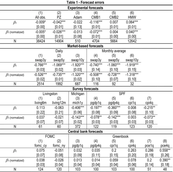
Table 1 presents the results of the estimation of equation (1) for our different types of measures and categories of agents. In order to make results more easily comparable, Table 1 also provides forecast errors normalized by the standard deviation of the predicted variable (i.e. the different measures of inflation). A significant coefficient indicates that the forecast is biased. A positive coefficient indicates that economic agents underestimate inflation.
Forecast errors are almost systematically negative in our sample of laboratory experiments: participants to laboratory experiments tend to overestimate inflation. However, there is some heterogeneity. In the data of Hommes, Massaro and Weber (2017) participants instead significantly underestimate inflation. In the sub-samples by Adam (2008) and Cornand and M’baye (2016), the error is not significant; however, as will become clear below from the analysis of absolute forecast errors, this is due to a compensation in errors.
The forecasts of financial market participants (extracted from inflation swaps) are always negative and significant. They increase with the horizon. Considering daily or monthly data does not affect these results. Similarly, forecast errors in the household sample are also negative and significant.
Forecast errors of professional forecasters exhibit a slightly less clear pattern: those regarding CPI for the next quarter (cpi1q) are not significant, while those for the next year (cpi4q) are. GDP price index forecasts for the current and next quarter (pgdp1q and pdgd4q) are also significant. We conclude that forecast errors of professional forecasters are most of the time negative and significant.
17 For evidence see, e.g., Roberts (1997), Croushore (1997), Thomas (1999), and more recently Mankiw et al. (2004), and
Mehra (2002). Notice however, that some authors point that the fact that expectations are apparently biased errors serially correlated, cannot be construed as evidence against the rational expectations hypothesis. Andolfatto et al.(2007) argue that the hypothesis of unbiasedness tends to be rejected in particular in small samples, but less often in larger samples and that it may be rational to be adaptive for agents when they cannot disentangle the effects of persistent and transitory shocks. Note finally that Romer and Romer (2000) observe that forecast rationality is insured after correcting for serial correlation, for almost all their data (except the Blue Chip sample, for which rationality is obtained when excluding Volcker disinflation). In our case, since some of the series exhibit forecast rationality, we do not control for serial correlation for comparability purposes so as to estimate the same regression specification in all cases.
By contrast, in the industry sample, forecast errors are not significant, whatever the horizon of the forecast (expectations at 6 months (living6m) and at 12 months (living12m)). Central bank forecasts are not significant either (except pce4q).
Table 1 - Forecast errors Experimental forecasts
(1) (2) (3) (4) (5) (6)
All obs. PZ Adam CMB1 CMB2 HMW
1 -0.009* -0.042*** -0.022 -0.116*** 0.007 0.064*** [0.00] [0.01] [0.13] [0.01] [0.01] [0.01] 1 (normalized) -0.005* -0.026*** -0.013 -0.072*** 0.004 0.040*** [0.00] [0.01] [0.08] [0.01] [0.00] [0.00] N 38424 14904 510 4704 5664 12642 Market-based forecasts
Daily Monthly average
(1) (2) (3) (4) (5) (6)
swap3y swap5y swap10y swap3y swap5y swap10y 1 -0.766*** -1.069*** -1.920*** -0.740*** -1.060*** -1.919*** [0.03] [0.02] [0.03] [0.14] [0.10] [0.15] 1 (normalized) -0.526*** -0.735*** -1.320*** -0.508*** -0.728*** -1.318*** [0.02] [0.01] [0.02] [0.10] [0.07] [0.10] N 2514 1992 687 116 92 32 Survey forecasts Livingston Michigan SPF (1) (2) (3) (4) (5) (6) (7)
living6m living12m mich1y pgdp1q pgdp4q cpi1q cpi4q 1 0.113 -0.063 -0.406*** -0.197** -0.360*** 0.008 -0.215**
[0.22] [0.21] [0.06] [0.08] [0.09] [0.08] [0.10]
1 (normalized) 0.037 -0,021 -0.143*** -0.078** -0.142*** 0.003 -0.073**
[0.07] [0.07] [0.02] [0.03] [0.03] [0.03] [0.03]
N 61 60 372 122 119 123 120
Central bank forecasts
FOMC Greenbook
(1) (2) (3) (4) (5) (6) (7) (8)
fomc_cy fomc_ny pgdp1q pgdp4q cpi1q cpi4q pce1q pce4q 1 0.075 -0.051 0.032 0.035 0.2 0.263 0.286 0.558**
[0.07] [0.08] [0.09] [0.11] [0.15] [0.20] [0.19] [0.26]
1 (normalized) 0.038 -0.026 0.013 0.014 0.059 0.078 0.2 0.390**
[0.03] [0.04] [0.04] [0.04] [0.04] [0.06] [0.14] [0.18]
N 124 120 103 100 103 100 51 48
Note: Standard errors in brackets. * p < 0.10, ** p < 0.05, *** p < 0.01. Parameters are obtained by estimating equation (1) with OLS. Market-based forecasts are considered at a daily or monthly frequency, Livingston has a semiannual frequency, Michigan monthly, SPF quarterly. FOMC and Greenbook are taken at a quarterly frequency. N is the size of each sample. For experimental data: PZ indicates data from Pfajfar and Zakelj (2018), Adam those from Adam (2008), CMB1 those from Cornand and M’baye (2018), CMB2 those from Cornand and M’baye (2016), and HMW those from Hommes, Massaro and Weber (2017). For market-based forecasts, the forecasting horizon is 3, 5 and 10 years. For surveys, the horizon for Livingston is 6 or 12 months, for Michigan 1-year, and for SPF 1-quarter and 4-quarter. For central bank forecasts, the horizon is the current and next calendar years for FOMC and 1-quarter and 4-quarter for Greenbook.
Table B provided in the Appendix performs robustness checks. Results exhibit less clear patterns for survey and central bank forecasts depending on the considered period. For a longer time period, forecast errors of industry and central bank become significant, while those of households and professional forecasters become insignificant.
Overall, comparing our different samples: SPF forecast errors (except cpi1q), financial market participants’ forecast errors, households’ and laboratory experiment forecasts are consistent and exhibit systematic errors: inflation is over-estimated. Forecasts obtained in laboratory experiments
exhibit lower errors. Central bank’s and industry’s forecasts exhibit no significant results. As will become clear below, considering absolute forecast errors qualifies such a result.
We secondly provide a robustness check of results from Table 1, by estimating the absolute forecast error. Our aim is to evaluate whether positive and negative errors possibly compensated each other and to determine the quality of forecasts for our different categories of agents and types of measures. The absolute forecast error at time t of inflation in period t+h is defined by: |FEt,t+h| ≡ |𝜋𝑡+ℎ − 𝜋̅̅̅̅̅̅̅̅|t+h\t . Following Romer and Romer (2000)18 and Ang, Bekaert, and Wei (2007) among
others, we test the following equation:
|FEt,t+h|= 𝛽2+ 𝜖𝑖𝑡 (2)
where 𝛽2 is the estimated constant, 𝜖𝑖𝑡is the error term (i stands for the six different categories of
economic agents) and the null hypothesis is: the estimated constant 𝛽2is not significantly different
from 0.
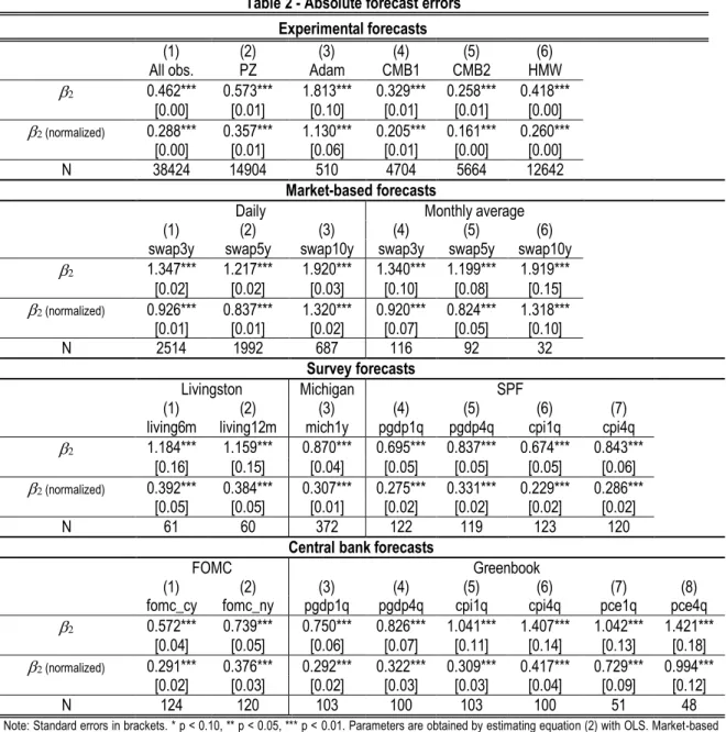
Table 2 provides estimates of equation (2) for our different samples. In order to make results more easily comparable, Table 2 also provides absolute forecast errors normalized by the standard deviation of the predicted variable (i.e. the different measures of inflation). A significant coefficient indicates that the absolute forecast error is significantly different from 0.
Table 2 shows that, considering absolute forecast errors, all forecast errors (that were not already significant in Table 1) become significant: experimental forecast errors become all significant, households’ forecast errors become significant even on a long period sample, industry’s forecast errors become significant even on the short 1990-2017 sub-period, professional forecast errors become all significant but there seems to be an inconsistency as swap3y errors are larger than swap5y (both for daily and monthly data). Also for SPF, we see that the CPI prevision is better than the GDP deflator at one year.19 In terms of accuracy (as evaluated by the average magnitude of absolute forecast errors),
forecast errors are comparable in our different data sets, especially when considering absolute forecast errors normalized by the standard deviation.20 They seem to be more pronounced for
market-based data and much less pronounced for experimental data (though the size of the sample may play a role).
Overall, the comparison between the analyses of forecast errors and absolute forecast errors enables us to formulate the following result:
Result 1: While forecast errors of participants to laboratory experiments, financial market participants, households and professional forecasters are systematically biased (i.e. forecasts exhibit over-evaluation of inflation on average), those from central bank and industry surveys are not. However, for each type of measure (experimental, survey, financial market and central bank data) and each category of economic agents, the forecast accuracy in terms of absolute forecast error is comparably large.
18 More precisely, Romer and Romer (2000) use the Mean Squared Errors (MSE) to estimate forecast accuracy, rather than
the absolute forecast error.
19 These results are robust to the considered period, as shown in Table C provided in the Appendix.
20 The fact that forecast errors are comparable also within the sample of experimental data is interesting. Because the designs
by Cornand and M’baye focus on central bank’s inflation target communication while other experimental designs do not, we could have expected more heterogeneity in forecast errors. Indeed, Dräger et al. (2016) make the link between consistent expectations, central bank communication and forecast accuracy. More precisely, they interpret consistency as effectiveness of central bank communication.
Table 2 - Absolute forecast errors Experimental forecasts
(1) (2) (3) (4) (5) (6)
All obs. PZ Adam CMB1 CMB2 HMW
0.462*** 0.573*** 1.813*** 0.329*** 0.258*** 0.418*** [0.00] [0.01] [0.10] [0.01] [0.01] [0.00] (normalized) 0.288*** 0.357*** 1.130*** 0.205*** 0.161*** 0.260*** [0.00] [0.01] [0.06] [0.01] [0.00] [0.00] N 38424 14904 510 4704 5664 12642 Market-based forecasts
Daily Monthly average
(1) (2) (3) (4) (5) (6)
swap3y swap5y swap10y swap3y swap5y swap10y 1.347*** 1.217*** 1.920*** 1.340*** 1.199*** 1.919*** [0.02] [0.02] [0.03] [0.10] [0.08] [0.15] (normalized) 0.926*** 0.837*** 1.320*** 0.920*** 0.824*** 1.318*** [0.01] [0.01] [0.02] [0.07] [0.05] [0.10] N 2514 1992 687 116 92 32 Survey forecasts Livingston Michigan SPF (1) (2) (3) (4) (5) (6) (7)
living6m living12m mich1y pgdp1q pgdp4q cpi1q cpi4q 1.184*** 1.159*** 0.870*** 0.695*** 0.837*** 0.674*** 0.843*** [0.16] [0.15] [0.04] [0.05] [0.05] [0.05] [0.06]
(normalized) 0.392*** 0.384*** 0.307*** 0.275*** 0.331*** 0.229*** 0.286***
[0.05] [0.05] [0.01] [0.02] [0.02] [0.02] [0.02]
N 61 60 372 122 119 123 120
Central bank forecasts
FOMC Greenbook
(1) (2) (3) (4) (5) (6) (7) (8)
fomc_cy fomc_ny pgdp1q pgdp4q cpi1q cpi4q pce1q pce4q 0.572*** 0.739*** 0.750*** 0.826*** 1.041*** 1.407*** 1.042*** 1.421***
[0.04] [0.05] [0.06] [0.07] [0.11] [0.14] [0.13] [0.18]
(normalized) 0.291*** 0.376*** 0.292*** 0.322*** 0.309*** 0.417*** 0.729*** 0.994***
[0.02] [0.03] [0.02] [0.03] [0.03] [0.04] [0.09] [0.12]
N 124 120 103 100 103 100 51 48
Note: Standard errors in brackets. * p < 0.10, ** p < 0.05, *** p < 0.01. Parameters are obtained by estimating equation (2) with OLS. Market-based forecasts are considered at a daily or monthly frequency, Livingston has a semiannual frequency, Michigan monthly, SPF quarterly. FOMC and Greenbook are taken at a quarterly frequency. N is the size of each sample. For experimental data: PZ indicates data from Pfajfar and Zakelj (2018), Adam those from Adam (2008), CMB1 those from Cornand and M’baye (2018), CMB2 those from Cornand and M’baye (2016), and HMW those from Hommes, Massaro and Weber (2017). For market-based forecasts, the forecasting horizon is 3, 5 and 10 years. For surveys, the horizon for Livingston is 6 or 12 months, for Michigan 1-year, and for SPF 1-quarter and 4-quarter. For central bank forecasts, the horizon is the current and next calendar years for FOMC and 1-quarter and 4-quarter for Greenbook.
A few remarks are in order. First, this result confirms the superiority of central bank’s forecasts already established in the literature.21 Romer and Romer (2000) – who compare the forecasting performance
of the Federal Reserve (using Greenbook data) and of commercial banks (using Blue Chip Economic Indicators, Data Resources, Inc. (DRI) and SPF) – show that the Federal Reserve better forecasts inflation than commercial forecasters.
Second, our first result qualifies the superiority of professional forecasts. The literature usually finds that professional forecasters stand in a better position than many other economic agents to forecast inflation (e.g. Carroll (2003)). Ang, Bekaert and Wei (2007) offer a comparison of four methods to study
21 Note however that this superiority should be taken with care as the number of observations is small. However, it is not
smaller than some of the other datasets (Livingston, SPF or monthly swaps for instance) and not smaller than equivalent samples in the literature.
inflation forecasting: time series forecasts, forecasts based on the Phillips curve, forecasts from the yield curve, and surveys (Livingston, Michigan, and SPF). Their comparison also shows the superiority of survey forecasts in forecasting inflation. Nevertheless, commenting such a result, they write (p. 1165): "That the median Livingston and SPF survey forecasts do well is perhaps not surprising, because presumably many of the best analysts use time-series and Phillips curve models. However, even participants in the Michigan survey who are consumers, not professionals, produce accurate out-of-sample forecasts, which are only slightly worse than those of the professionals in the Livingston and SPF surveys.” Our results are in line with this comment and extends it to experimental data.
Third, our first result emphasizes the performance comparability of laboratory data to various categories of field data: experimental forecasts are biased as other data and are not less accurate than other data.
3.2. Informational frictions and up-date frequency
We analyze whether our different economic agents are subject to informational frictions when forecasting inflation and how they up-date their information. Is there some heterogeneity in these respects for our different categories of agents? To answer these questions, following Coibion and Gorodnichenko (2012), we evaluate for our different categories of economic agents whether forecast errors are autocorrelated, whether they depend on forecast revisions, and whether forecast revisions depend on past forecast revisions. If they are, this means that economic agents do not incorporate all available information. Instead, if forecast errors are not predictable, economic agents use all the information they have and are in particular able to up-date their information set between two periods. First of all, to study the potential autocorrelation of forecast errors, wetest the following equation:
FEt,t+h= 𝐶1+ 𝛽3FEt−1,t+h−1𝑖+ 𝜖𝑖𝑡 (3)
where 𝛽3 is the estimated coefficient, 𝐶1 is a constant, 𝜖𝑖𝑡is the error term (i stands for the six different
categories of economic agents) and the null hypothesis is: the estimated coefficient 𝛽3is not
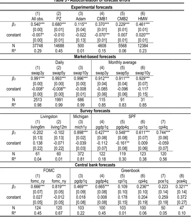
significantly different from 0. Table 3 provides estimations of equation (3) for our different samples. A significant coefficient indicates that forecast errors are autocorrelated.
Theoretically, in a frictionless world, forecast errors should not be correlated to previous forecast errors. However, in the sticky information model (Mankiw and Reis, 2002), "forecast errors depend both on the inflation process after the shock and on the degree of information rigidity. […] As the degree of information rigidity rises, conditional forecast errors will become increasingly persistent." (Coibion and Gorodnichenko, 2012, p. 122). There is much evidence in the literature that they are. For example, Diebold (1989) shows that inflation forecast errors are typically serially correlated and hence predictable. Romer and Romer (2000, p. 433) also show that "the serial correlation increases as the horizon for the forecasts becomes longer." However, more recently, evidence is mixed. Coibion and Gorodnichenko (2012) show that "forecast errors are not predictable using lagged inflation conditional on lagged forecast errors".
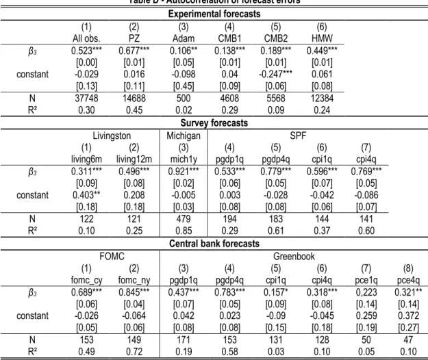
Table 3 shows that forecast errors are indeed autocorrelated: the forecast error is predictable owing to the former error, suggesting that economic agents do not form rational expectations. This characteristic is robust over almost all our samples (with only a few exceptions: Industry data (Livingston), Greenbook data (cpi1q and pce1q)). Note that Table D reported in Appendix shows that for a longer period of time, autocorrelation of forecast errors on industry data also become significant. In terms of amplitude, market-based forecast errors seem to be more autocorrelated, while
Greenbook data exhibit less autocorrelation in forecast errors (although one should be careful in interpretation because coefficients are biased by the frequency of the sample). Considering fixed effects for experimental data does not yield further insights.
Table 3 - Autocorrelation of forecast errors Experimental forecasts
(1) (2) (3) (4) (5) (6)
All obs. PZ Adam CMB1 CMB2 HMW
β3 0.540*** 0.680*** 0.115** 0.370*** 0.229*** 0.461*** [0.00] [0.01] [0.04] [0.01] [0.01] [0.01] constant -0.007* -0.010 -0.022 -0.070*** 0.007 0.020*** [0.00] [0.01] [0.13] [0.01] [0.01] [0.01] N 37748 14688 500 4608 5568 12384 R² 0.29 0.45 0.01 0.15 0.06 0.23 Market-based forecasts
Daily Monthly average
(1) (2) (3) (4) (5) (6)
swap3y swap5y swap10y swap3y swap5y swap10y β3 0.991*** 0.993*** 0.996*** 0.912*** 0.911*** 0.929*** [0.00] [0.00] [0.00] [0.04] [0.04] [0.07] constant -0.008* -0.008** -0.008 -0.085 -0.096 -0.117 [0.00] [0.00] [0.01] [0.06] [0.06] [0.15] N 2513 1991 686 115 91 31 R² 0.98 0.99 0.99 0.85 0.83 0.85 Survey forecasts Livingston Michigan SPF (1) (2) (3) (4) (5) (6) (7)
living6m living12m mich1y pgdp1q pgdp4q cpi1q cpi4q β3 -0.202 -0.102 0.898*** 0.427*** 0.548*** 0.611*** 0.744*** [0.13] [0.13] [0.02] [0.08] [0.08] [0.07] [0.06] constant 0.138 -0.071 -0.039 -0.112 -0.161** 0.009 -0.059 [0.22] [0.22] [0.03] [0.07] [0.08] [0.06] [0.07] N 61 60 372 122 119 123 120 R² 0.04 0.01 0.81 0.18 0.30 0.38 0.56
Central bank forecasts
FOMC Greenbook
(1) (2) (3) (4) (5) (6) (7) (8)
fomc_cy fomc_ny pgdp1q pgdp4q cpi1q cpi4q pce1q pce4q β3 0.666*** 0.819*** 0.469*** 0.665*** 0.109 0.236** 0.223 0.321** [0.07] [0.05] [0.09] [0.08] [0.10] [0.10] [0.14] [0.14] constant 0.027 -0.012 0.018 0.008 0.178 0.204 0.259 0.372 [0.05] [0.05] [0.08] [0.08] [0.15] [0.19] [0.19] [0.27] N 124 120 103 100 103 100 50 47 R² 0.45 0.67 0.22 0.45 0.01 0.06 0.05 0.10 Note: Standard errors in brackets. * p < 0.10, ** p < 0.05, *** p < 0.01. Parameters are obtained by estimating equation (3) with OLS. Market-based forecasts are considered at a daily or monthly frequency, Livingston has a semiannual frequency, Michigan monthly, SPF quarterly. FOMC and Greenbook are taken at a quarterly frequency. N is the size of each sample. For experimental data: PZ indicates data from Pfajfar and Zakelj (2018), Adam those from Adam (2008), CMB1 those from Cornand and M’baye (2018), CMB2 those from Cornand and M’baye (2016), and HMW those from Hommes, Massaro and Weber (2017). For market-based forecasts, the forecasting horizon is 3, 5 and 10 years. For surveys, the horizon for Livingston is 6 or 12 months, for Michigan 1-year, and for SPF 1-quarter and 4-quarter. For central bank forecasts, the horizon is the current and next calendar years for FOMC and 1-quarter and 4-quarter for Greenbook.
Second, we analyze whether forecast errors are predictable owing to forecast revisions. The forecast revision at time t of inflation in period t+h is defined by: FRt,t+h≡ 𝜋̅̅̅̅̅̅̅̅ − 𝜋t+h\t ̅̅̅̅̅̅̅̅̅̅̅̅̅̅t+h−1\t−1. We estimate
the following equation (equivalent to equation (11) in Coibion and Gorodnichenko (2012)):
where 𝛽4 is the estimated coefficient, 𝐶2 is a constant, 𝜖𝑖𝑡is the error term (i stands for the six different
categories of economic agents) and the null hypothesis is: the estimated coefficient 𝛽4is not
significantly different from 0. If there is no informational friction, forecast errors should theoretically not be correlated to forecast revisions.
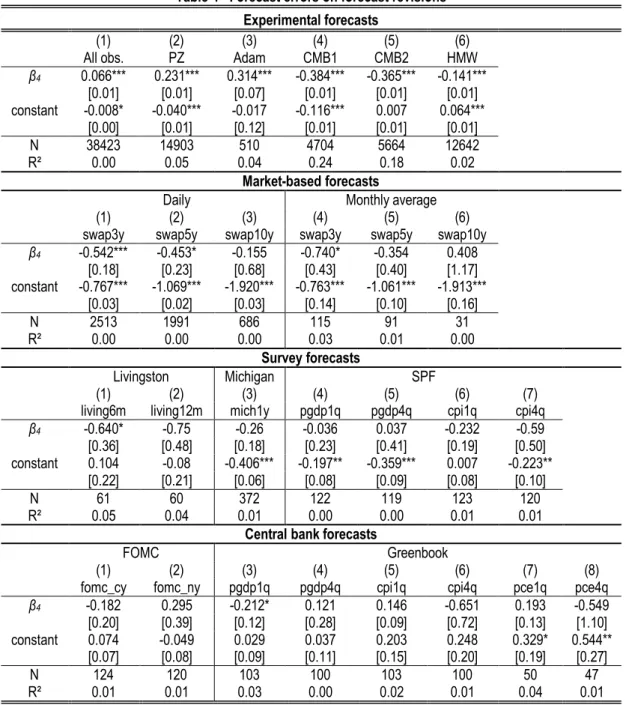
Table 4 provides estimates of equation (4) for our different samples. A significant coefficient indicates that the error is predictable owing to the revision.
Errors of professional forecasters and central bankers (except pdgp1q) are not predictable (as for financial market participants on long horizons) owing to forecast revision, meaning that they tend to use more available information than other economic agents. By contrast, coefficients are significant in the samples of laboratory participants, industry (except linving6m) and to some extend for financial market participants (especially swap3y).22 Data from laboratory experiments are thus relatively
comparable to financial market participants’ data in this respect (although the amplitude is even more pronounced for market-based data).
However, there is some heterogeneity among our samples and within the sample of experiments in terms of signs. When economic agents revise their expectations upward between t-1 and t, this reduces their forecast error in industry data (when significant, i.e. on the 1956-2017 period as presented in Table E of the Appendix) and for the experiment by Pfajfar and Zakelj and Adam, but increases their forecast error in Cornand and M’baye and in Hommes, Massaro and Weber,23 in
household data (over a long time period as exposed in table E in Appendix) and in financial market data on short horizons.
Tables H and I provided in Appendix give additional precisions to Table 4 by providing a decomposition between current and lagged inflation forecasts following equation (12) in Coibion and Gorodnichenko (2012). In particular, in the case where previous Table 4 does not exhibit significant results, one can see whether one of the two (current and lagged inflation forecasts) is significant. Theoretically, without informational friction, they should not be (Coibion and Gorodnichenko, 2012). The main result of Table 4 is confirmed by Tables H and I reported in the Appendix.24
22 It seems that both industry and household data are more reliable in the recent period than in the past, as Table E in
Appendix shows that over a longer period, forecast errors on forecast revisions on industry and household data become significant when they were not on a shorter period or even more significant when they were already significant.
23 Considering fixed effects does not alter the results regarding experimental data as shown in Table E reported in the
Appendix.
24 Only lagged expected inflation is significant, with a negative sign for household data; expected inflation in living6m is
significant with a negative sign for industry data; regarding central bank’s forecast, lagged expected inflation is significant on Greenbook data for pgdp4q, cpi1q, pce1q.
Table 4 - Forecast errors on forecast revisions Experimental forecasts
(1) (2) (3) (4) (5) (6)
All obs. PZ Adam CMB1 CMB2 HMW
β4 0.066*** 0.231*** 0.314*** -0.384*** -0.365*** -0.141*** [0.01] [0.01] [0.07] [0.01] [0.01] [0.01] constant -0.008* -0.040*** -0.017 -0.116*** 0.007 0.064*** [0.00] [0.01] [0.12] [0.01] [0.01] [0.01] N 38423 14903 510 4704 5664 12642 R² 0.00 0.05 0.04 0.24 0.18 0.02 Market-based forecasts
Daily Monthly average
(1) (2) (3) (4) (5) (6)
swap3y swap5y swap10y swap3y swap5y swap10y β4 -0.542*** -0.453* -0.155 -0.740* -0.354 0.408 [0.18] [0.23] [0.68] [0.43] [0.40] [1.17] constant -0.767*** -1.069*** -1.920*** -0.763*** -1.061*** -1.913*** [0.03] [0.02] [0.03] [0.14] [0.10] [0.16] N 2513 1991 686 115 91 31 R² 0.00 0.00 0.00 0.03 0.01 0.00 Survey forecasts Livingston Michigan SPF (1) (2) (3) (4) (5) (6) (7)
living6m living12m mich1y pgdp1q pgdp4q cpi1q cpi4q β4 -0.640* -0.75 -0.26 -0.036 0.037 -0.232 -0.59 [0.36] [0.48] [0.18] [0.23] [0.41] [0.19] [0.50] constant 0.104 -0.08 -0.406*** -0.197** -0.359*** 0.007 -0.223** [0.22] [0.21] [0.06] [0.08] [0.09] [0.08] [0.10] N 61 60 372 122 119 123 120 R² 0.05 0.04 0.01 0.00 0.00 0.01 0.01
Central bank forecasts
FOMC Greenbook
(1) (2) (3) (4) (5) (6) (7) (8)
fomc_cy fomc_ny pgdp1q pgdp4q cpi1q cpi4q pce1q pce4q β4 -0.182 0.295 -0.212* 0.121 0.146 -0.651 0.193 -0.549 [0.20] [0.39] [0.12] [0.28] [0.09] [0.72] [0.13] [1.10] constant 0.074 -0.049 0.029 0.037 0.203 0.248 0.329* 0.544** [0.07] [0.08] [0.09] [0.11] [0.15] [0.20] [0.19] [0.27] N 124 120 103 100 103 100 50 47 R² 0.01 0.01 0.03 0.00 0.02 0.01 0.04 0.01 Note: Standard errors in brackets. * p < 0.10, ** p < 0.05, *** p < 0.01. Parameters are obtained by estimating equation (4) with OLS. Market-based forecasts are considered at a daily or monthly frequency, Livingston has a semiannual frequency, Michigan monthly, SPF quarterly. FOMC and Greenbook are taken at a quarterly frequency. N is the size of each sample. For experimental data: PZ indicates data from Pfajfar and Zakelj (2018), Adam those from Adam (2008), CMB1 those from Cornand and M’baye (2018), CMB2 those from Cornand and M’baye (2016), and HMW those from Hommes, Massaro and Weber (2017). For market-based forecasts, the forecasting horizon is 3, 5 and 10 years. For surveys, the horizon for Livingston is 6 or 12 months, for Michigan 1-year, and for SPF 1-quarter and 4-quarter. For central bank forecasts, the horizon is the current and next calendar years for FOMC and 1-quarter and 4-quarter for Greenbook.
We can thus conclude that in contrast to professional and central bankers’ forecasts, for households and industry, forecast errors are predictable owing to forecast revisions (though less than for the other samples), and in the same direction as in the financial market participant sample, as well as in the same direction of some of the experimental sub-samples.
Thirdly, we evaluate whether forecast revisions can be predicted owing to past forecast revisions. More precisely, the question we answer is whether economic agents revise their expectations upwards if the former forecast is revised upwards. To this aim, we test the following equation:
FRt,t+h= 𝐶3+ 𝛽5FRt−1,t+h−1+ 𝜖𝑖𝑡 (5) where 𝛽5 is the estimated coefficient, 𝐶3 is a constant, 𝜖𝑖𝑡is the error term (i stands for the six different
categories of economic agents) and the null hypothesis is: the estimated coefficient 𝛽5is not
significantly different from 0.
Forecast revisions should theoretically not be correlated to lagged forecast revisions, as there is no reason for economic agents to always revise their forecasts in the same direction.
Table 5 presents estimations of equation (5) for our different samples. A significant and positive coefficient indicates that economic agents revise their expectations upwards if the former forecast is revised upwards. The table exhibits significant coefficients (except for households, swap10y for financial market participants on monthly data, pgdp4q for professional forecasters and most central bank’s forecasts). The sign is generally negative (except for Pfajfar and Zakelj’s and Hommes, Massaro and Weber’s sub-samples in experimental data).
Table F in Appendix overall confirms this analysis on longer periods, except for industry data that become non-significant and household data that become significant.25
Overall, regarding information frictions, we can state the following result:
Result 2: For each type of measure and each category of agents at the notable exception of central bank data, inflation forecasts are subject to information rigidities.
(a) Forecast errors are highly autocorrelated for all types of measure (experimental, survey, financial market, and central bank data) and each category of agents except industry forecasters.
(b) Forecast errors are predictable owing to forecast revisions – indicating that economic agents are unable to up-date their information between periods – except for central bank and professional forecasters.
(c) Lagged forecast revisions enter significantly and usually negatively in forecast revisions for all types of measures and each category of agents – indicating that economic agents alternate revising their expectations upwards and downwards –, except for central bank data.
Our second result calls for some comments. First, our result confirms previous studies pointing to evidence of information frictions. In particular, our results are in line with those of Andrade and Le Bihan (2013) who – relying on the European Central Bank Survey of Professional Forecasters – show that forecasters fail to update their forecasts and have predictable forecast errors. As argued by Coibion and Gorodnichenko (2012, p. 136), "because professional forecasters are some of the most informed economic agents, […] any evidence of information rigidity on their part [is] particularly notable". Our result also goes in the direction of those of Romer and Romer (2000) emphazising the idea that staff and policymakers from the Fed form better forecasts than professional (commercial) forecasters.
25 Considering fixed effects does not alter the results regarding experimental data as shown in Table F reported in the
Table 5 - Forecast revisions on lagged forecast revisions Experimental forecasts
(1) (2) (3) (4) (5) (6)
All obs. PZ Adam CMB1 CMB2 HMW
β5 0.078*** 0.258*** -0.156*** -0.471*** -0.441*** 0.051*** [0.01] [0.01] [0.04] [0.01] [0.01] [0.01] constant -0.001 -0.008 -0.011 -0.019 0.001 0.019*** [0.00] [0.01] [0.08] [0.01] [0.01] [0.01] N 37748 14687 500 4608 5568 12385 R² 0.01 0.07 0.02 0.25 0.21 0.00 Market-based forecasts
Daily Monthly average
(1) (2) (3) (4) (5) (6)
swap3y swap5y swap10y swap3y swap5y swap10y β5 -0.310*** -0.223*** -0.268*** -0.353*** -0.278*** -0.103 [0.02] [0.02] [0.02] [0.08] [0.08] [0.08] constant 0 0 0 -0.009 -0.007 -0.006 [0.00] [0.00] [0.00] [0.02] [0.02] [0.01] N 3295 3295 3295 150 150 150 R² 0.10 0.05 0.07 0.12 0.08 0.01 Survey forecasts Livingston Michigan SPF (1) (2) (3) (4) (5) (6) (7)
living6m living12m mich1y pgdp1q pgdp4q cpi1q cpi4q β5 -0.466*** -0.432*** -0.075 -0.188** -0.126 -0.230** -0.176** [0.11] [0.12] [0.05] [0.09] [0.09] [0.09] [0.09] constant -0.025 -0.032 -0.001 -0.009 -0.014 -0.011 -0.015 [0.07] [0.05] [0.02] [0.03] [0.02] [0.04] [0.02] N 62 62 373 124 124 124 124 R² 0.22 0.19 0.01 0.04 0.02 0.05 0.03
Central bank forecasts
FOMC Greenbook
(1) (2) (3) (4) (5) (6) (7) (8)
fomc_cy fomc_ny pgdp1q pgdp4q cpi1q cpi4q pce1q pce4q β5 0.004 -0.039 -0.408*** -0.173* -0.237** 0.014 -0.218 0.122 [0.09] [0.09] [0.09] [0.10] [0.10] [0.10] [0.14] [0.14] constant -0.004 -0.007 -0.014 -0.015 -0.029 -0.021 -0.045 -0.013 [0.03] [0.02] [0.07] [0.04] [0.15] [0.03] [0.20] [0.03] N 124 124 104 104 104 104 50 50 R² 0.00 0.00 0.17 0.03 0.06 0.00 0.05 0.02 Note: Standard errors in brackets. * p < 0.10, ** p < 0.05, *** p < 0.01. Parameters are obtained by estimating equation (5) with OLS. Market-based forecasts are considered at a daily or monthly frequency, Livingston has a semiannual frequency, Michigan monthly, SPF quarterly. FOMC and Greenbook are taken at a quarterly frequency. N is the size of each sample. For experimental data: PZ indicates data from Pfajfar and Zakelj (2018), Adam those from Adam (2008), CMB1 those from Cornand and M’baye (2018), CMB2 those from Cornand and M’baye (2016), and HMW those from Hommes, Massaro and Weber (2017). For market-based forecasts, the forecasting horizon is 3, 5 and 10 years. For surveys, the horizon for Livingston is 6 or 12 months, for Michigan 1-year, and for SPF 1-quarter and 4-quarter. For central bank forecasts, the horizon is the current and next calendar years for FOMC and 1-quarter and 4-quarter for Greenbook.
Second, in spite of differences in economic context (long vs. short period of time, including data from a potentially less vs. more transparent period of time) and design regarding experimental data sets (for exemple, with vs. without communication about a forward-looking variable such as the central bank target in Cornand and M’baye vs. Pfajfar and Zakelj and Hommes, Massaro and Weber) that could have induced more or less informational frictions, our results are relatively consistent within samples. The most important heterogeneity in results is observed when regressing forecast errors on forecast
revisions (Result 2 (b)) and can possibly be attributed to these differences in economic context and design.26
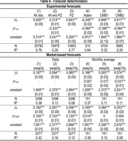
3.3. Forecast determination
Are inflation forecasts’ determinants the usual ones (namely lagged inflation and output gap) for each of our different categories of economic agents? To answer this question, in line with e.g. Lanne et al. (2009), Fendel et al. (2010), and Dräger et al. (2016), we test the following equation:
𝜋t+1\t
̅̅̅̅̅̅̅̅ = 𝐶4+ 𝛽6𝜋𝑡−1+ 𝛽7𝑦𝑡+ 𝜖𝑖𝑡 (6) where 𝛽6 and 𝛽7 are the estimated coefficients, 𝑦𝑡 denotes the output gap in period t, 𝐶4 is a constant, 𝜖𝑖𝑡 is the error term (i stands for the six different categories of economic agents). Based on the
standard Phillips curve relationship, we expect inflation forecasts to be determined by lagged inflation and output gap.
Table 6 - Forecast determination Experimental forecasts
(1) (2) (3) (4) (5) (6)
All obs. All w/o PZ PZ Adam CMB1 CMB2
6 0.928*** 0.314*** 0.943*** -0.248*** 0.646*** 0.617*** [0.00] [0.01] [0.00] [0.02] [0.03] [0.01] OG . -0.333*** . -0.560*** -0.390*** -0.064*** [0.01] [0.02] [0.02] [0.01] constant 0.314*** 3.437*** 0.200*** 4.973*** 1.845*** 1.884*** [0.01] [0.05] [0.02] [0.09] [0.13] [0.07] N 25782 10879 14903 510 4704 5665 R² 0.76 0.26 0.77 0.64 0.32 0.28 Market-based forecasts
Daily Monthly average
(1) (2) (3) (4) (5) (6)
swap3y swap5y swap10y swap3y swap5y swap10y
6 0.187*** 0.094*** 0.060*** 0.188*** 0.093*** 0.074*** [0.00] [0.00] [0.00] [0.02] [0.02] [0.02] OG . . . 0.001 -0.017 -0.031** [0.02] [0.02] [0.01] constant 1.949*** 2.375*** 2.664*** 1.929*** 2.372*** 2.631*** [0.01] [0.01] [0.01] [0.05] [0.05] [0.04] N 3296 3296 3296 151 151 151 R² 0.38 0.13 0.08 0.37 0.11 0.11 6 0.182*** 0.091*** 0.056*** 0.169*** 0.084*** 0.053*** [0.00] [0.00] [0.00] [0.02] [0.02] [0.02] GDP 0.155*** 0.102*** 0.120*** 0.015** 0 0.004 [0.01] [0.01] [0.01] [0.01] [0.01] [0.01] constant 1.951*** 2.377*** 2.666*** 1.957*** 2.390*** 2.670*** [0.01] [0.01] [0.01] [0.05] [0.05] [0.04] N 3277 3277 3277 151 151 151 R² 0.42 0.16 0.12 0.39 0.10 0.08 (continued)
26 Over a longer time period, including data from a less transparent period of time, economic agents (household and industry)
might have been more backward than forward-looking, which may impede them using potentially available information and thus make more accurate forecasts. The same kind of reasoning can be applied to experimental data. Indeed, in contrast to participants in Adam’s and Pfajfar and Zakelj’s experiments, participants in the experiments by Cornand and M’baye where in some treatments provided with the inflation target of the central bank, which possibly induced more forward-looking behavior.