CAEPR Working Paper #014-2009
Why do Education Vouchers Fail?
Peter Bearse, Buly A. Cardak, Gerhard Glomm, B. Ravikumar
Indiana University
August 16, 2009
This paper can be downloaded without charge from the Social Science Research Network electronic library at: http://ssrn.com/abstract=1456391.
The Center for Applied Economics and Policy Research resides in the Department of Economics at Indiana University Bloomington. CAEPR can be found on the Internet at:
http://www.indiana.edu/~caepr. CAEPR can be reached via email at [email protected] or via phone at 812-855-4050.
©2008 by NAME. All rights reserved. Short sections of text, not to exceed two paragraphs, may be quoted without explicit permission provided that full credit, including © notice, is given to the source.
Why do Education Vouchers Fail?
Peter Bearse
yBuly A. Cardak
zGerhard Glomm
xB. Ravikumar
{August 16, 2009
Abstract
We examine quantitatively why uniform vouchers have repeatedly su¤ered electoral defeats against the current system where public and private schools coexist. We argue that the topping-up option available under uniform vouchers is not su¢ ciently valuable for the poorer households to prefer the uniform vouchers to the current mix of public and private education. We then develop a model of publicly funded means-tested edu-cation vouchers where the voucher received by each household is a linearly decreasing function of income. Public policy, which is determined by majority voting, consists of two dimensions: the overall funding level (or the tax rate) and the slope of the means testing function. We solve the model when the political decisions are sequential – households vote …rst on the tax rate and then on the extent of means testing. We establish that a majority voting equilibrium exists. We show that the means-tested voucher regime is majority preferred to the status-quo. These results are robust to alternative preference parameters, income distribution parameters and voter turnout.
We are thankful for helpful comments from Marco Basetto, V.V. Chari, Gianni De Fraja, Rich Romano, Jon Sonstelie, Itzhak Zilcha and seminar participants at Ben Gurion University, Tel Aviv University, The Federal Reserve Bank of Minneapolis and the University of Illinois. This paper has also bene…tted from comments received at the Meeting of the Society for Economic Dynamics in San Jose, Costa Rica, the Winter Meetings of the Econometric Society in Atlanta, GA, the CEPR/IHS Conference on Dynamic Aspects of Policy Reform in Vienna, Austria and the Public Economic Theory meetings in Galway, Ireland. Any remaining shortcomings are entirely our own.
yDepartment of Economics, 462 Bryan School of Business and Economics, University of North Carolina
at Greensboro, Greensboro, NC 27402-6165, [email protected]
zSchool of Economics and Finance, La Trobe University, Victoria 3086, Australia,
xCorresponding author: Department of Economics, Wylie Hall, Room 105, Indiana University,
Bloom-ington, IN 47405, [email protected]
{Department of Economics, Pappajohn Business Building, University of Iowa, Iowa City, IA 52242,
1
Introduction
In the year 2000, two U.S. states — California and Michigan — put proposals for large scale, statewide education vouchers on their ballots. Both proposals were soundly rejected in statewide elections, with opposition at the ballot box in excess of 60%. These two cases are the most well known in a string of electoral defeats involving vouchers. This phenomenon is not limited to the U.S.; education vouchers of scope greater than that of an experimental level are rare in other countries as well. (West (1997) and Carnoy (1997) provide descriptions and di¤ering interpretations of these experiments.) The coexistence of public and private education seems to be the predominant institutional arrangement (see James, 1987).
In this paper, we examine the political support for (or opposition to) education vouchers. To illustrate our …ndings, we use the model of Epple and Romano (1996) and Glomm and Ravikumar (1998) as our benchmark education …nance regime. In that model, both public and private schools coexist. All households pay income taxes to fund public education, but they can opt out of public education to attend a private school of their choice at their own cost. The funding level for public education in this mixed public-private regime is determined by majority voting. We compare the benchmark against a uniform voucher economy similar to the one recommended by Friedman (1962). In our voucher economy, the government collects taxes on income and uses the tax revenue to …nance education vouchers. Each school age child receives the same voucher amount. Unlike the status-quo mix of public and private education, the government does notprovideeducation in our voucher economy; it only
…nances education. Given the voucher amount each child receives, households determine the level of educational services for their children. Some households use their after-tax income to supplement vouchers (and reduce their consumption/other goods), while others do not. The amount of public funding for the vouchers is determined through majority voting.
Both regimes, the status-quo mix of public and private education as well as the uniform vouchers, impose lower bounds on the educational expenditures of each household. However,
the uniform voucher regime provides households the option of “topping up” whereas the status-quo does not. When we switch from the status-quo to the uniform vouchers, the size of the pie (i.e., the tax rate) as well as the distribution of the pie changes. For a household whose allocation in the status-quo is such that the marginal rate of substitution (MRS) of education for other goods is greater than the marginal rate of transformation (MRT) i.e., for the relatively rich households, the topping-up option might have positive value and might a¤ect the political support for the status-quo. However, poor households in our setup are typically faced with the opposite situation where their MRS is less than the MRT and the topping-up option does not have positive value. The magnitude of the change in the tax rate and the number of households who are better o¤ with the topping-up option are clearly important for the support for vouchers.
We calibrate the status-quo mixed education regime to match the U.S. data. We then change the regime to a uniform voucher economy and calculate the new equilibrium values. (We think of this as a constitutional reform, where the regime is switched once and for all.) The uniform voucher regime yields a higher equilibrium tax rate relative to the status-quo (5:34% vs. 5:18%). We then conduct an election between the status-quo and uniform vouchers. We …nd that the uniform voucher regime is unable to garner a majority of the votes. This …nding is robust to various plausible changes in parameters for preferences and income distribution. Under our parameterization, the bottom68% of the income distribution stands to lose from switching to uniform vouchers. The cross-sectional distribution of welfare gains/losses reveals that the bottom68% su¤er a welfare loss of slightly less than one percent of their income whereas some rich households gain as much as three percent.
To isolate the e¤ect of the distribution of the pie, we compare the two regimes by …xing the size of the pie to be the same as that in the status-quo (by …xing the tax rate at the status-quo level of 5:18%). With the same tax rate, the rich households who chose private education in the status-quo would be better o¤ since part of the cost of private education is o¤set by the voucher. The poor households receive a smaller voucher than the educational
expenditure in the status-quo since the tax revenues are distributed among all households in the uniform voucher regime instead of among just those who chose public education. Despite the lower voucher amount some households could take advantage of the topping-up option in the uniform voucher regime if the overall resources available to them are su¢ ciently large and if their consumption-voucher bundle is such that their MRS is greater than the MRT. Quantitatively, however, it turns out that for the lower part of the income distribution the topping-up option does not make them better o¤ relative to the status-quo, either because the overall resources are not su¢ ciently large or because their MRS is less than the MRT. Consequently, even with the same tax rate, a majority of households prefer the status-quo to uniform vouchers.
Since the opposition to uniform vouchers is mainly from the poorer households, a natural alternative is to consider means-tested vouchers. By distributing the pie progressively instead of uniformly, the opposition to vouchers could potentially be reduced. To examine the alternative, we develop a model of means-tested vouchers where the voucher amount is decreasing linearly in income.1 As in the case of uniform vouchers, some households use
their after-tax income to supplement the vouchers, while others do not. In our means-tested voucher model, public policy is two-dimensional: (i) the overall funding level for the voucher program and (ii) the extent of means testing, i.e., the tax rate and the slope of the means testing function. Both policy variables are endogenously determined through majority voting. (Note that the uniform voucher is a special case of this model where the means-testing rate is set to zero.) We determine political outcomes sequentially in order to avoid well-known existence problems associated with multidimensional voting; see Ordeshook (1986, Chapter 4.7). We assume households …rst vote on the tax rate, followed by a vote on the means testing rate. When households vote on the tax rate, they anticipate the majority
decision rule for means testing that follows in the sequence. For this voting sequence, we
1Many public subsidies around the world are targeted or means–tested (see van de Walle and Nead,
1995). A number of the small-scale, experimental voucher programs in the US are means tested, such as the program in Milwaukee.
prove the existence and uniqueness of a majority voting equilibrium.
Quantitatively, we …nd that the means-tested voucher regime yields a lower equilibrium tax rate relative to the status-quo mix of public and private education (4:48% vs. 5:18%). In the election between the status-quo and the tested vouchers, we …nd that the means-tested voucher regime is chosen by a majority of voters. This majority consists of a coalition of the rich and poor. Again, this result is robust to di¤erent plausible parameterizations of the preferences and income distribution. When we switch from the status-quo to means-tested vouchers, the bottom45% and the top17% gain roughly one percent of their income. When we …x the tax rate in the means-tested regime at the status-quo level of5:18%, the poor households receive a larger voucher relative to the educational expenditure in the status-quo and a majority prefers the means-tested vouchers to the status-quo.
Our sensitivity analysis also considers the case where voter participation in elections depends on income. In the U.S., the probability of voting increases with income. We recalibrate the status-quo mixed education model to the U.S. education data as well as voter participation data. Our main results are qualitatively unchanged. First, a uniform voucher regime is unable to garner a majority of the votes relative to the status-quo and, second, a means-tested voucher regime is preferred to the status-quo by a majority.
Finally, for the means-tested vouchers, we consider “simultaneous voting” on the tax and means testing rates, as in Shepsle (1979), instead of sequential voting (in the voting literature, this case is referred to as “voting one dimension at a time” or “issue by issue voting”). Again, our conclusions are qualitatively unchanged.
In related work, Chen and West (2000) study both uniform and targeted education vouchers.2 In their means-tested (selective) voucher model, all households with income below
a threshold receive the same voucher amount whereas households with higher income receive no voucher at all. In equilibrium, only households with incomes less than or equal to that of
2Other work on education vouchers includes Hoyt and Lee (1998), Nechyba (1999, 2000), Rangazas (1995),
Cohen-Zada and Justman (2003, 2005), Ferreyra (2007) and Bearse, Glomm and Ravikumar (2000). For a study of other institutional arrangements in education see, for example, Fernandez and Rogerson (2003).
the decisive voter in the mixed public-private school regime receive a voucher. They …nd the mixed regime is preferred to the uniform voucher regime while the decisive voter is indi¤erent between their selective voucher and the mixed regimes. When they assume that the mixed regime is ine¢ cient at delivering educational services relative to a voucher regime i.e., a unit of tax revenue yields more education in the voucher regime than in the mixed regime, they …nd that their selective voucher regime is majority preferred to the mixed regime. The latter conclusion depends heavily on the presumed production ine¢ ciency in their model. We have no production ine¢ ciency in our model and, yet, we …nd that means-tested vouchers are majority preferred to the mixed regime whereas uniform vouchers are not.3
The structure of our paper is the following. In Section 2, we develop our model of means-tested vouchers. Uniform vouchers are a special case of this model. In Section 3 we prove that a sequential majority voting equilibrium exists for our model. We also prove the existence of and characterize the majority voting equilibrium for the case of uniform vouchers. In Section 4, we calibrate the status-quo mixed public-private education regime to match features of the U.S. data. We then conduct computational experiments to examine the popular support and the distribution of welfare gains for the di¤erent voucher regimes relative to the status-quo. Section 5 examines the sensitivity of our results to alternative levels of voter participation, preference parameters and income distribution parameters and to simultaneous voting over the tax and means testing rates. Concluding remarks are contained in Section 6. Proofs are relegated to Appendix A.
2
Model
In this section, we describe a model of means-tested vouchers. The model of uniform vouchers is a special case of the means-tested vouchers model where the means testing rate is set to
3As the evidence on improvements in student outcomes arising from the introduction of large scale
vouchers is mixed, we choose to exclude such e¤ects from our model. For some of this evidence see Angrist et al. (2002) on Colombia, Brunello and Checchi (2005) on Italy, Figlio and Rouse (2006) and Rouse et al. (2007) on the US state of Florida, Filer and Munich (2000) on the Czech Republic and Hungary, Ladd and Fiske (2000, 2001) on New Zealand, Parry (1997) and Hsieh and Urquiola (2006) on Chile, and Sandström and Bergström (2005) on Sweden.
zero. The means-tested vouchers model has two variables chosen via majority voting whereas the uniform vouchers model has only one.
The economy is populated by a large number of households. We normalize the size of the population to 1. Households di¤er only by income, y, which is endowed across households according to the c.d.f. F (p.d.f. f); the p.d.f. is assumed to be continuously di¤erentiable. We label households by their income and refer to a household with incomey as “household
y”. The support of F is R+ and mean income, Y, exceeds median income,ym.
Households derive utility from a numeraire consumption good cand a good e which we refer to as education. The common utility function is u(c; e) which is strictly increasing in both arguments, strictly quasiconcave, and twice continuously di¤erentiable. We follow Epple and Romano (1996) and impose the following:
Assumption 1. For c1 >0; e1 >0; c2 0; and e2 0,
u(c1; e1)>maxfu(c2;0); u(0; e2)g:
The market foreis assumed to be perfectly competitive with a large number of producers facing identical technologies exhibiting constant marginal costs. We measure units of e so as to normalize its price to one unit of consumption. Both consumption and education are assumed to be normal goods.
The government collects a tax on income at the rate 2[0;1]. Total tax revenue is given by Y. All tax revenue is used to …nance education vouchers which are means-tested in the sense that the voucher amount depends inversely on income and there is an income threshold above which a household receives no voucher. Formally, the voucher amount for household
y is given by
v(y; ; ) = maxf y;0g; 0; 0: (1)
0 implies uniform vouchers. We assume that the government runs a balanced budget; i.e.,
Z 1
0
v(y; ; )f(y)dy= Y:
Equivalently, since the voucher amount is 0 for a household with income larger than , we can write the balanced budget restriction as
F
Z
0
yf(y)dy = Y: (2)
We refer to (2) as the Government Budget Constraint (GBC) and lete( ; )be the value of satisfying(2)given ( ; ). Note that in a uniform voucher regime each household receives the voucher amount v, so we can write the government budget constraint as v = Y.4
2.1
Household Optimization
Each household treats ; ; and as given and chooses the pair (c; e) so as to maximize utility u(c; e) subject to the budget constraint
c+e (1 )y+v(y; ; ); c (1 )y: (3)
Denote the optimal choices of household y bybc(y; ; ; ) and be(y; ; ; )and the indirect utility of household y byV (y; ; ; ) u(bc(y; ; ; );be(y; ; ; )).
Remark 1. In cases where = 0 or = 1; no household obtains a voucher and all
educational expenditures are privately …nanced. When = 0, the GBC requires = 0; no household receives a voucher. When = 1, (3) implies that all households get zero consumption. Assumption 1 will rule this out as a potential equilibrium.
Household y supplements its voucher if and only if
@u((1 )y+v(y; ; ) e; e)
@e e=v(y; ; ) >0
4As noted in the Introduction, both uniform vouchers and means-tested vouchers are merely instruments
used by the government to …nance education; the government does not directly provide education. In our model of vouchers, a “school” is similar to a “…rm” in the neoclassical model that converts resources to education, so terms such as “public schools” are meaningless.
or, equivalently,
R(y) u1((1 )y; v(y; ; ))
u2((1 )y; v(y; ; ))
<1
where the subscripts here denote partial derivatives of u. Put di¤erently, there exists a threshold income such that household y supplements its voucher if and only if y exceeds the threshold. We further restrict preferences to ensure that, for income distributions with support on the real line, there exist low income households who do not supplement their voucher as well as rich households who do supplement their voucher.
Assumption 2. For all >0; 2(0;1); and 2(0;1); (i) limy&0R(y)>1, and,
(ii) limy%1R(y)<1:
2.2
Politico-Economic Equilibrium
The voting problem in this means-tested voucher regime involves two variables, and . Once these are determined, the value of is pinned down by GBC (2). We determine the pair ( ; ) through majority voting in two stages. In the …rst stage, individuals vote on the tax rate anticipating how the means testing parameter will be chosen in the second stage and how might depend on . In the second stage, is voted on taking from the …rst stage as given. We de…ne a politico-economic equilibrium for this voting sequence as follows.
De…nition 1. Apolitico-economic equilibriumfor the means-tested vouchers economy is an allocation (c; e) across households and a public policy ( ; ; ) satisfying (i) Each household’s choice of (c; e) is individually rational given public policy( ; ; ); (ii) Given ,
is a majority winner in the second stage; (iii) Anticipating how a¤ects voting over , is a majority winner in the …rst stage; and, (iv) The government runs a balanced budget; i.e., = e( ; ).
We de…ne majority voting in the usual sense of binary comparisons between all policies. We treat voters as sincere in that they will vote for the policy that yields a higher utility in
any binary comparison between policies.5 We say that a policy is amajority winner at each
stage if and only if no other policy satisfying the GBC at that stage is strictly preferred to it by a strict majority of the population.
In the case of uniform vouchers, household y’s budget constraint is the same as (3) except that the voucher amount is independent of y i.e., set v(y; ; ) = v in (3). The voting problem has only one variable, . The equilibrium for the uniform voucher economy is de…ned below.
De…nition 2. Apolitico-economic equilibriumfor the uniform vouchers economy is an allocation (c; e) across households and a public policy (v; ) satisfying (i) Each household’s choice of (c; e) is individually rational given public policy (v; ); (ii) is a majority winner; and, (iii) The government runs a balanced budget; i.e.,v = Y.
3
Majority Voting Equilibrium
As noted earlier, the households in our model have to collectively choose two policy variables – and – sequentially. In this section, we establish the existence of a majority voting equilibrium for our means-tested voucher model and characterize the equilibrium. We also establish the existence of and characterize the majority voting equilibrium for the uniform voucher model.
3.1
Voting over Means Testing
Here we solve the problem of voting over . At this stage, the households have already voted on a tax rate and the problem is to choose (collectively) a means testing rate. However, we have to take into account the fact that in voting over the tax rate, households would have considered the e¤ect of each tax rate on the subsequent election for . To this end, we have to determine the majority preferred for each . Household y chooses
5In this section, we assume that all households actually vote. In our computational experiments below,
to maximize the indirect utility subject to (2): Formally, given 2 (0;1), her optimal is arg max V (y;e( ; ); ; ):
Remark 2. When = 0, there are no vouchers and the choice of is irrelevant. The case
= 1can never occur in equilibrium since every household would get zero consumption and, as noted before, this is ruled out by Assumption 1.
Since is given, the size of the pie to be redistributed is …xed. Since our means testing formula bestows larger amounts to poorer households, no household above mean income Y
will bene…t from this formula and they will all prefer = 0. Support for a positive means testing rate must then come from households whose incomes are below the mean. The following proposition characterizes the extent of means testing preferred by the majority.
Proposition 1. (Majority preferred ) The household with the median income (ym) is the
decisive voter. Given 2(0;1); b( ) is a majority winner where b solves
ym =
@e( ; )
@ :
In deciding the means testing rate, the decisive voter has to choose a pair ( ; ) among the pairs that satisfy the GBC. In the ( ; ) space, the GBC is concave as illustrated in Figure 1. To understand the trade-o¤s faced by each voter receiving a voucher, consider an arbitrary householdy whose income is less thanY (recall that households withy Y prefer
= 0). Suppose that household y is constrained by the voucher amount in the sense that its consumption is(1 )y and its educational expenditure is y. Then, on the margin, any increase in has to be o¤set by an increase in to keep this household indi¤erent. More precisely, every unit increase in would require an increase in by y units. So, in the ( ; ) space, the slope of the indi¤erence curve for household y is y. Now, suppose that householdy is not constrained by the voucher amount in which case the household will optimally allocate its resources (1 )y+ y between consumption and educational expenditures. (Recall that the optimal choices are denoted by bc and be.) On the margin,
α β GBC slope= y slope= y′< y
Y
τ
0 0 y α β− =Figure 1: GBC and Indi¤erence Curves of households.
a unit increase in decreases this household’s utility by yfu1(bc;be) +u2(bc;be)g whereas a
unit increase in increases this household’s utility by fu1(bc;be) +u2(bc;be)g. To keep the
household indi¤erent, has to increase byy units for every unit increase in . Again, in the
( ; )space, the slope of the indi¤erence curve for household y is y, as illustrated in Figure 1. The preferred( ; ) pair for householdy is clearly where its indi¤erence curve is tangent to the GBC. (Note from Figure 1 that the tangency point implies y >0.) Proceeding along the same lines, a poorer householdy0 < y would have a ‡atter indi¤erence curve in the
( ; )space and would, hence, prefer a higher( ; )pair. Thus, the preferred means testing rate is a decreasing function of income –richer households prefer a lower , with households above the mean income preferring = 0. This monotonicity allows us to invoke the median voter theorem and establish Proposition 1.
To determine the majority preferred tax rate, we have to characterize the function b( )
in Proposition 1 i.e., we have to understand how the majority preferred changes as the tax rate changes. To this end, the following properties of the GBC are helpful.
Lemma 1. (Properties of GBC) Fix 2(0;1)and let( ; )be a point on the GBC. Denote this GBC as GBC1. Consider another GBCj with tax rate j = j 2 (0;1). Then, (i) the
pair (j ; j ) is on GBCj and (ii) the slope of GBCj at (j ; j ) is the same as the slope of
GBC1 at( ; ).
Lemma 1 characterizes the set of feasible ( ; ) pairs that constrains household ym for
each : For every change in , proportionate changes in and are in the feasible set, according to part (i). Part (ii) implies that household ym would indeedchoose the
propor-tionate change. That is, if ( ; ) was the most preferred pair for household ym on GBC1,
then (j ; j ) is its most preferred pair on GBCj. Thus, the functional relation between the
majority preferred and the tax rate can be characterized as follows.
Proposition 2. (Decision rule for the majority preferred and ) b( ) =k
for some constant k > 0 for all 2 (0;1): Furthermore, associated with b( ), the unique b( ) e( ; k ) that satis…es the GBC can be written as
b( ) =k for some constant k >0:
Among the pairs ( ; ) that satisfy the GBC, the majority preferred pair establishes an extensive margin that excludes some households from receiving any portion of the pie (households withy bb = kk ). A natural question then is, does the extensive margin change as the size of the pie changes (i.e., as the tax rate and, hence, the GBC changes)? According to Proposition 2, the answer is no. As the tax rate changes, the majority preferred ( ; )
pairs must have the property that is constant. In turn, this implies the identities of the households that are excluded from receiving vouchers are invariant to the tax rate. Put di¤erently, no matter what the size of the pie is, the pie is always distributed between the
3.2
Voting over the Tax Rate
To determine the majority preferred , each household takes as given the majority preferred
functions b( ) and b( ) given by Proposition 2 and chooses its most preferred . With a slight abuse of notation, householdy chooses to
maxV (y; ) V (y;k ; k ; ):
We will …rst establish that the households’ preferences over are single-peaked. It is easy to see that households above the income level kk would prefer a tax rate of zero since they do not receive any voucher at all. Furthermore, their utility is monotonically declining in the tax rate, so V (y; ) peaks at = 0 for y > kk . The set of households whose utilities are declining in the tax rate is, in fact, larger. Consider all households who receive positive vouchers and whose voucher amount is less than what they pay in taxes. The set of such households is given by fy: 0< y < yg or fy: 0< k k y < yg. The critical household for which the voucher exactly o¤sets taxes is y = k
1+k , so for y > k
1+k , it is
clear that (i) the most preferred tax rate would be zero and (ii) the household’s utility is monotonically declining in since the gap between taxes and bene…ts ( y (k k y)) is increasing in (or, the total resources available to household y are decreasing in ). In Appendix A, we prove that households with y < 1+kk also have single-peaked preferences, so we have the following proposition.
Proposition 3. (Majority preferred existence) Given b( )and b( )from Proposition 2, households’preferences over are single-peaked and, hence, there exists a majority voting equilibrium tax rate.
Since the households with incomes above 1+kk prefer a zero tax rate, for the equilibrium tax rate to be positive, the decisive voter must come from the group y < 1+kk . Denote the decisive voter’s income byyd. The lemma below states necessary conditions for the majority
Lemma 2. (Properties of ) Suppose that the majority preferred tax rate is positive. Then, (i) the decisive voter’s income yd 2
h
0;1+kk i, (ii) The most preferred tax rate b(yd) of
the decisive voter is such that the decisive voter is constrained i.e., his consumption and educational expenditure are given by
b
c= (1 b(yd))yd; be=k b(yd) k b(yd)yd;
(iii) The most preferred tax rateb(yd) is the unique solution to
u2((1 )yd; k k yd) u1((1 )yd; k k yd) = yd k k yd : Slope = -1 Slope y kα k yβ = − c e 1 k y k α β < + ,τ τ′ < . kατ−kβτy
( )
1−τ y(
1−τ′)
y+kατ′−kβτ′y( )
1−τ y+kατ−kβτyFigure 2: Tradeo¤s for the decisive voter
The decisive voter, if unconstrained by the voucher amount, can make himself better o¤ with a higher tax rate. Higher implies more resources, but a tighter constraint on e (or
c). For an increase of ; he gains k k y y > 0 units of resources, which translates into higher c and e since he is not constrained, as illustrated in Figure 2. He
can increase the tax rate until he is constrained, at which point the increase in would imply less consumption and his marginal rate of substitution of consumption for educational expenditure is no longer equal to 1. However, he can continue to increase the tax rate and make himself better o¤ until he reaches the equality in part (iii) of Lemma 2.
What remains to be determined is who is the decisive voter. To this end, we restrict the preferences further to the constant relative risk aversion (CRRA) class. Let
u(c; e) = 8 > < > : 1 1 (c 1 + e1 ); >0; 6 = 1; >0; lnc+ lne; = 1: (4)
For this class of preferences, the proposition below pins down the decisive voter and the majority voting equilibrium. We will use these preferences in the next section for our quan-titative analysis.
Proposition 4. (Majority preferred for CRRA utility) Let u(c; e) be speci…ed according to (4). If 1;then the decisive voter is household ym and the majority preferred tax rate
is given by (k k ym) ((1 )ym) = ym k k ym : (5)
If >1;then the decisive voter is implicitly determined by
1 F k
1 +k +F (yd) = 0:5 (6)
and the majority preferred tax rate is given by
(k k yd) ((1 )yd) = yd k k yd :
3.3
Uniform Vouchers
In the uniform voucher regime, every household gets a voucher amount equal to Y. House-hold y’s budget constraint is similar to (3):
Letbcandbebe the optimal choices and let V(y; )be the indirect utility of householdy: The voting problem for each household here is one dimensional. The proposition below is the counterpart to the results in the previous subsection.
Proposition 5. (Uniform Vouchers majority preferred ) (i) Households’preferences over are single-peaked and there exists a majority voting equilibrium tax rate. (ii) For the equilibrium tax rate to be positive, the decisive voter’s income yU
d is less than Y, the most
preferred tax rateb(yU
d)of the decisive voter is such that
bc= 1 b(yUd) ydU; eb=b(ydU)Y; and b(yU
d) is the unique solution to
u2 (1 )ydU; Y u1((1 )ydU; Y) = y U d Y :
(iii) Let u(c; e) be speci…ed according to (4). If 1; then the decisive voter is household ym and the majority preferred tax rate is given by
( Y) ((1 )ym)
= ym
Y ;
and if >1; then the decisive voter is implicitly determined by 1 F (Y) +F yU
d = 0:5
and the majority preferred tax rate is given by
( Y) ((1 )yU d) = y U d Y :
Part (iii) of Proposition 5 is described in detail in Glomm and Ravikumar (1995).
4
Are Vouchers Electable?
In this section, we examine quantitatively whether vouchers can garner a majority of the votes when compared with the status-quo mixed public-private education regime of Epple and Romano (1996) and Glomm and Ravikumar (1998). We choose the mixed public-private regime as our benchmark since it is a good description of the current K-12 education system in the U.S. In this regime, households can opt out of public education, sending their children
Parameters Variables Matched
m= 3:36
s= 0:68
Model U.S. Data Median Income $28,789 $28,906 Mean Income $36,257 $36,250
= 1:54 = 0:02
Model U.S. Data
Public Education Expenditure
per Public Household $2,126 $2,111 Implied Price Elasticity of
Demand for Public Education -0.67 -0.67
Table 1: Calibrated values for model parameters
to private schools instead, albeit at their own cost. For completeness, we provide a brief description of this discrete-choice model in Appendix B.
We consider two voucher regimes – uniform and means-tested – as alternatives to the status-quo. To implement our quantitative analysis, we assume a lognormal(m; s2)income
distribution, and we parameterize the utility function described in (4). With these functional forms, we pin downmands2directly from the data on household income distribution. Hence,
we have only two preference parameters, and , to calibrate.
We choose m = 3:36 and s = 0:68 to match the mean and median incomes in the U.S. household income distribution in 1989, measured in thousands of dollars. Recall that the vouchers were defeated at the polls in California and Colorado in 1992 and again in California and Michigan in 2000. We choose = 1:54and = 0:02to match public funding per public pupil of$4;222 in the 1989 U.S. data (assuming0:5pupils per household) and an implied price elasticity of demand for public education equal to 0:67.6 The values of the
calibrated parameters are presented in Table 1. These values imply that the bottom88% of the households choose public education and the top 12% opt out, which is consistent with the school enrollment data.
6Solution techniques for the mixed and uniform voucher regimes are well known. (See Epple and Romano,
1996, and Glomm and Ravikumar, 1995.) Our approach to solving for equilibrium (see de…nition 1) in the means-tested voucher regime is described in Bearse, Glomm and Ravikumar (2000).
4.1
Status-Quo Versus Vouchers
For the benchmark, we consider the case where all households vote. (We will consider incomplete participation where the probability of voting is an increasing function of income in Section 5 and show that the results on the electability of vouchers are unchanged.) Voting equilibria are summarized in Table 2 and the outcomes of pairwise elections over education funding regimes are presented in Table 3.
Tax Rate Public expenditure or Voucher Mixed Education 5.18% $2,126
Uniform Voucher 5.34% $1,936 Means-Tested Voucher 4.48% $(3244 0:0492y)
Table 2: Voting equilibria for the three education …nancing regimes.
M-T Vouchers vs. Mixed 62.2% for M-T Vouchers M-T Vouchers vs. Uniform Vouchers 56.7% for M-T Vouchers
Uniform Vouchers vs. Mixed 31.4% for Uniform Vouchers Table 3: Binary voting comparisons
The uniform voucher involves a higher tax compared to the mixed education status-quo (5:34% versus5:18%), but each household receives a voucher less than the public expenditure in the status-quo ($1;936versus$2;126). The lower voucher amount occurs because the tax revenues in the mixed regime are distributed only among the 88 percent of the population who choose public education whereas in the uniform voucher regime the tax revenues are distributed among all households. Households with incomes below the43rd percentile choose not to supplement the voucher. For these households, the status-quo o¤ers higher consump-tion (since the tax rate is lower) and higher educaconsump-tional expenditure (since they don’t opt out), so they are strictly better o¤ in the status-quo. The lower tax rate in the status-quo suggests that households choosing private education might be better o¤, but the uniform voucher regime o¤ers$1;936as a lump sum to these households whereas the status-quo o¤ers zero. For the very rich households (above the99th percentile), however, the higher after-tax income in the status-quo more than o¤sets the uniform voucher amount. These households
will also be strictly better o¤ in the status-quo. As shown in Table 3, the status-quo is preferred to the uniform voucher regime by a majority.
The means-tested voucher regime o¤ers lower taxes relative to the status-quo (4:48% versus 5:18%). The parameters of the means testing function in Table 2 imply that almost every household that chose private education in the status-quo receives zero voucher. Almost all of the tax revenues in the means-tested voucher economy are distributed among the
88 percent of the households that chose public education in the status-quo regime. For households with incomes below the 36th percentile, it also o¤ers a voucher greater than the status-quo public expenditure. The lower tax plus a higher voucher will certainly make the households below the 36th percentile strictly better o¤ in the means-tested regime. Furthermore, the means-tested regime will receive support from all households above the88th percentile in the income distribution since these households opted out of public education and faced higher taxes in the status-quo. Finally, continuity suggests that the means-tested regime will also garner support from some households slightly above the36th percentile and slightly below the88th percentile. As a result, the means-tested regime is majority preferred to the status-quo.
Comparing the uniform voucher regime to the means-tested voucher regime, households pay less taxes in the latter (5:34% versus4:48%). Households with incomes below the 45th percentile receive a higher voucher amount in the latter; these households are strictly better o¤ in the means-tested regime. The lower tax rate implies that each household’s after-tax income increases by 0:86% in the means-tested regime. In contrast, some households receive zero vouchers in the means-tested regime whereas all households receive $1;936 in the uniform voucher regime. Again, for the very rich households, the increase in after-tax income in the means-tested regime more than o¤sets the voucher amount in the uniform regime. Consequently, these households also strictly prefer the means-tested regime. The combination of lower taxes and higher voucher amounts imply that the means-tested regime will defeat the uniform voucher regime at the polls. In the next subsection, we provide details
on the winners and losers as we switch from the status-quo to the two voucher regimes.
4.2
Who Wins And Who Loses?
In this subsection, we report the cross-sectional distribution of welfare gains of adopting a means-tested or uniform voucher regime. To provide a welfare metric that is invariant to monotonic transformations of the utility function, we consider dev that solves
VM ix(y(1 +dev)) = VN ew(y) (7)
whereVM ix(y(1 +d
ev))denotes the utility that a household with incomey(1 +dev)receives
in the mixed public-private equilibrium and VN ew(y) indicates the utility that household y
obtains in equilibrium under the proposed voucher regime. The equivalent variationdev
rep-resents the income transfer, measured in percent, that would make household y indi¤erent between the mixed public-private regime and the proposed voucher regime. When dev is
positive, household y would be worse o¤ in the status-quo mixed regime without the com-pensating variation. The proposed voucher regime then represents a welfare improvement from the household’s perspective anddev quanti…es the magnitude of the welfare gain. Figure
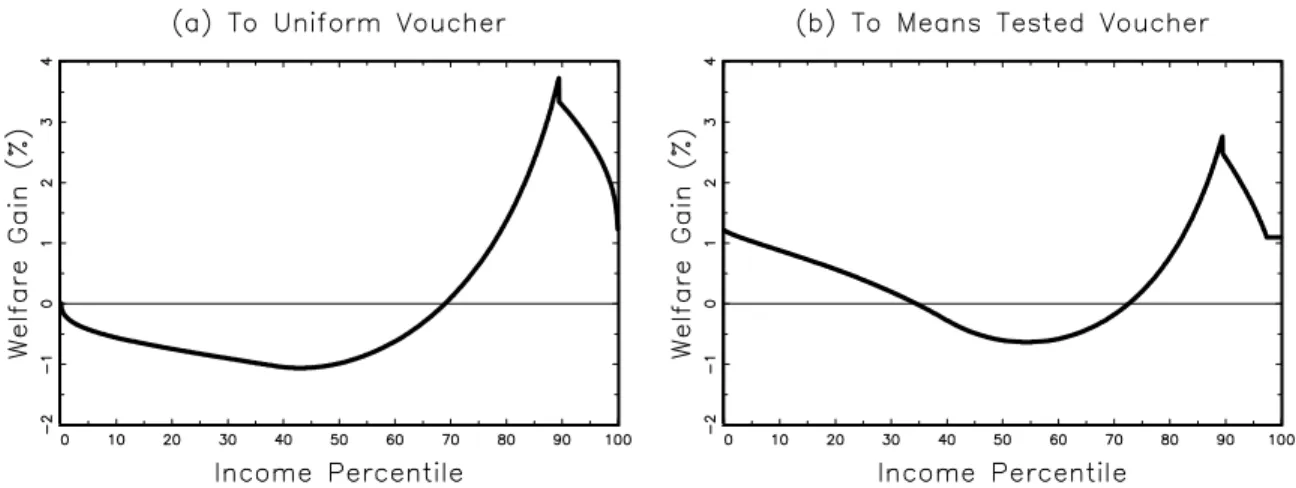
3 depicts the gains and losses.
Figure 3: Welfare gains to switching from the mixed public-private regime.
Our computations reveal that switching from the mixed regime to uniform vouchers imparts welfare losses to the poorest 68% of the population. It should be noted that while
only the top 12% choose private education in the mixed regime, almost the entire top 32% prefer the higher tax and the uniform voucher since they can supplement the voucher and attain higher utility. The welfare losses to the bottom68% are less than one percent of their income, but the welfare gains to some of the richer households exceed three percent.
It is the middle to upper-middle income households who lose under means-testing. For instance, households between the 45th and the 83rd income percentiles would be willing to give up to one percent of their income to remain in the status-quo.
4.3
Political Support with Exogenous Tax
As noted in the Introduction, the voucher regimes o¤er a “topping up” option whereas the status-quo does not. Despite the option, we …nd that the uniform vouchers lack the political support to abandon the status-quo. In the previous subsections, the size of the pie as well as the distribution of the pie changes as we switch from the status-quo to the uniform voucher regime. In this subsection, we isolate the e¤ect of the distribution of tax revenues, holding the tax rate …xed.
We compare the status-quo against uniform vouchers when the tax rate is …xed at the same level as that in the status-quo (5:18%). Thus, the constraint on consumption is iden-tical in both regimes: c (1 )y. For the households who chose public education in the status-quo, the voucher amount is less than the educational expenditure in the status-quo. This is because the tax revenues are distributed among all households in the uniform voucher regime whereas in the status-quo only those who chose public education receive the tax rev-enues. Even though the voucher amount is lower, some households (e.g., the relatively rich) might be better o¤ if their consumption-voucher bundle is such that their marginal rate of substitution of education for consumption is greater than the marginal rate of transforma-tion. Such households could use the topping-up option to increase educational expenditure by reducing their consumption, making themselves better o¤, provided the overall resources available to them are su¢ ciently large. On the other hand, for households at a bundle where
the marginal rate of substitution of education for consumption is less than the marginal rate of transformation, the topping-up option has no value. This is typically the case for the households below the 41st percentile in our model as illustrated in Figure 4; these house-holds cannot move in the direction of less educational expenditure and more consumption. Households between41st and 68th percentiles …nd the topping-up option valuable, but their overall resources are not large enough to achieve an allocation superior to what they had in the status-quo. Thus, even with the same tax rate, it turns out that the bottom 68% prefer the status-quo to the uniform vouchers.
e c (1-τ)y τY τY/N (1-τ)y+α−βy (1-τ)y+τY α−βy
Figure 4: Tradeo¤s for a poor household with an exogenous tax rate
In the means-tested regime, however, the voucher exceeds educational expenditure in the status-quo for most households who chose public education. In fact, the topping-up option has no value for the bottom 49% of the households, but they are clearly better o¤ in the means-tested regime, as illustrated in Figure 4. The topping-up option is valuable to the rest of the households, but for a few of these households the resources are not large enough to dominate the allocation they had in the status-quo. As a result, a majority of households
support the switch from the status-quo to the means-tested regime, even when the tax rate is exogenous.
Both empirical evidence (the 1992 referenda in California and Colorado and the 2000 referenda in California and Michigan) and views commonly expressed in the popular press promote the widespread belief that vouchers are not politically viable. Our results support this claim with respect to uniform vouchers. On the other hand, our …ndings suggest that an appropriate means-tested voucher regime could generate a majority backing. As noted earlier, this result is not driven by presumed production e¢ ciency gains in the public sector induced by competition from vouchers.
5
Sensitivity Analysis
In this section, we examine whether our results presented in Sections 4.1 and 4.2 are robust to alternative parameterizations about voter participation, preferences, income distribution and to an alternative voting mechanism.
5.1
Incomplete Voter Participation
In contrast to Section 4 where all households vote in the election, here we consider the case where the probability of voting is an increasing function of income. We use data from the
1990 Statistical Abstract of the United States to assign voting probabilities. Table 4 displays voter participation by income quintile.7 Within quintiles, we assume that the probability of
voting is constant.
Income Quintile 1 2 3 4 5
Proportion Voting 0.40 0.48 0.56 0.64 0.72
Table 4: Voting Turnout by Income Quintile
Voting equilibria are summarized in Table 5. With partial voter turnout, results are similar to the complete participation case except that the uniform voucher involves a lower
7Solving for equilibria in this case is identical to that where all households vote, except that the identity
tax than the status-quo along with a much lower voucher. Table 6 presents the results for pairwise elections across regimes. We see that the means-tested vouchers are majority preferred to both the mixed regime and to uniform vouchers. Furthermore, the mixed regime is majority preferred to uniform vouchers.
Tax Rate Public expenditure or Voucher Mixed Education 5.44% $2,205
Uniform Voucher 4.94% $1,791 Means-Tested Voucher 4.40% $2379 0:0222y
Table 5: Voting equilibria for the three education regimes with incomplete voter participa-tion.
M-T Vouchers vs. Mixed 60.9% for M-T Vouchers M-T Vouchers vs. Uniform Vouchers 52.9% for M-T Vouchers
Uniform Vouchers vs. Mixed 38.4% for Uniform Vouchers Table 6: Binary Voting Comparisons with incomplete voter participation
Figure 5: Welfare Gains to switching from the Mixed Public-Private Regime with incomplete voter participation.
Figure 5 illustrates the welfare gains/losses as in Section 4.2. As before, we see that it is the middle to upper-middle income households who lose under means-testing. When voter participation is an increasing function of income, one noteworthy di¤erence to the case of complete participation is that the size of the welfare gains from shifting to the means-tested are smaller for the poor, but larger for the rich.
5.2
Preferences
In this subsection, we examine di¤erent values for the preference parameters and while maintaining the benchmark lognormal(3:36;0:682) income distribution. We consider four
sets of values for ( ; ), each roughly matching public education expenditure per household of $2;111 and one of four implied price elasticities of education demand when evaluated at the mixed regime equilibrium. These values are displayed in Table 7.
Implied Price Elasticity of Education Demand 2.200 0.006 -0.500
1.540 0.020 -0.670 0.790 0.111 -1.250 0.650 0.155 -1.500
Table 7: Alternative Preference Parameter Values
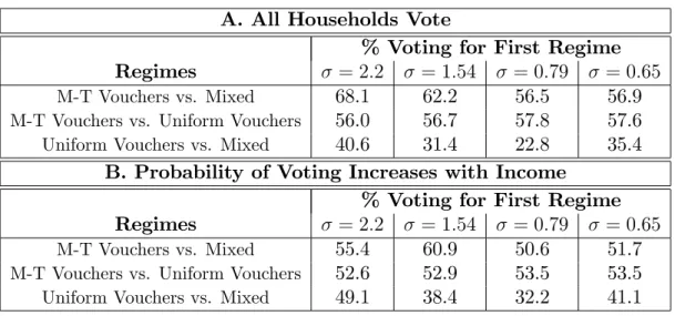
In panels A and B of Table 8, we again present the results for pairwise elections. We see that, for both sets of voting populations and each set of preference parameters, means-tested vouchers are majority preferred to both the mixed public-private regime and to uniform vouchers. Also in every case, the mixed regime is majority preferred to uniform vouchers.
A. All Households Vote
% Voting for First Regime
Regimes = 2:2 = 1:54 = 0:79 = 0:65
M-T Vouchers vs. Mixed 68.1 62.2 56.5 56.9
M-T Vouchers vs. Uniform Vouchers 56.0 56.7 57.8 57.6
Uniform Vouchers vs. Mixed 40.6 31.4 22.8 35.4
B. Probability of Voting Increases with Income % Voting for First Regime
Regimes = 2:2 = 1:54 = 0:79 = 0:65
M-T Vouchers vs. Mixed 55.4 60.9 50.6 51.7
M-T Vouchers vs. Uniform Vouchers 52.6 52.9 53.5 53.5
Uniform Vouchers vs. Mixed 49.1 38.4 32.2 41.1 Table 8: Binary Voting Comparisons for alternative preference parameters
5.3
Income Distribution
We now change the parameters of the income distribution while maintaining our bench-mark preference parameter values of = 1:54 and = 0:02. Under the lognormal income distribution, mean income is given by Y = exp (m+s2=2). We …x mean income at Y = exp (3:36 + 0:682=2)' 36:278 and perform mean-preserving spreads of the income distribu-tion using m = 3:36 + 0:682=2 s2=2 for the values of s displayed in Table 9. The di¤erent combinations of s and m imply the same mean income, but di¤erent median incomes. (As
s m Median y Gini 0.430 3.499 $33,072 0.239 0.680 3.360 $28,789 0.385 0.930 3.159 $23,540 0.489
Table 9: Mean-Preserving Spreads of Income Distribution
is well-known for the lognormal distribution, inequality is increasing ins.) Table 10 displays the results. We see that our principal …ndings are robust to variations in income inequal-ity. In particular, while uniform vouchers are unable to defeat the status-quo at the polls, means-tested vouchers consistently garner a majority of the votes, against the status-quo as well as against uniform vouchers.
A. All Households Vote
% Voting for First Regime
Regimes s= 0:43 s= 0:68 s= 0:93
M-T Vouchers vs. Mixed 57.7 62.2 64.1
M-T Vouchers vs. Uniform Vouchers 55.3 56.7 57.3
Uniform Vouchers vs. Mixed 37.2 31.4 30.0
B. Probability of Voting Increases with Income % Voting for First Regime
Regimes s= 0:43 s= 0:68 s= 0:93
M-T Vouchers vs. Mixed 63.3 60.9 60.2
M-T Vouchers vs. Uniform Vouchers 50.2 52.9 54.7
Uniform Vouchers vs. Mixed 47.9 38.4 36.2
5.4
Simultaneous Voting
In this subsection, we consider an alternative to the sequential voting mechanism described in Section 2.2. We examine a “simultaneous voting” mechanism where both the extent of means testing and the tax rate are voted on iteratively instead of sequentially.8 This is
achieved through a structure induced equilibrium, as de…ned in Shepsle (1979) and discussed in Ordeshook (1986, pp. 245-57). In a two-issue space, the structure assumes a vote over issue 1 while issue 2 is …xed. After the …rst vote, issue 1 is …xed at the majority winner of the …rst vote and a vote is conducted over issue 2. This process is repeated until aninvulnerable
voting equilibrium is identi…ed.
Here thepolitico-economic equilibrium is as de…ned in Section 2.2 except for the political aspects given by parts (ii) and (iii) of De…nition 1. These are replaced by: (ii) The chosen policy pair ( ; ) is invulnerable in the sense that, given no other feasible is preferred by a majority to and conversely, given no other is preferred by a majority to .
The sincerity of voting, perfect foresight, balanced budget and majority winner requirements discussed in Section 2.2 are retained.
The majority preferred for each is the same as the means testing rate studied in Section 3.1, so ( ) = k . We derive the majority preferred for each numerically. We calibrate the model as in Section 4 and for the benchmark parameters, we plot the majority preferred for each in Figure 6. The unique …xed point in this …gure is the structure induced politico-economic equilibrium for the benchmark parameters. The equilibrium values are = 3:66% and = 4:02%. The base voucher is = $2;651 while the threshold income for a zero voucher is $65;829 (89th percentile).
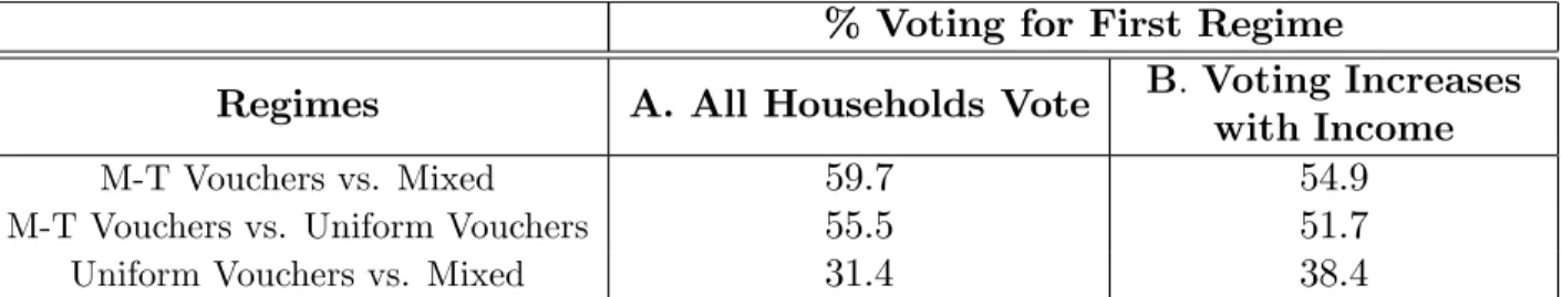
We now turn to the results of pairwise elections between the di¤erent voucher regimes and the status-quo. Table 11 makes comparisons similar to Table 3 and comes to similar qualitative conclusions. The status-quo and uniform voucher regimes have not changed
8The terminology in the literature for the mechanism described in this subsection is “voting one dimension
Figure 6: Voting equilibrium under simultaneous voting.
% Voting for First Regime
Regimes A. All Households Vote B: Voting Increases
with Income
M-T Vouchers vs. Mixed 59.7 54.9
M-T Vouchers vs. Uniform Vouchers 55.5 51.7
Uniform Vouchers vs. Mixed 31.4 38.4
Table 11: Binary Voting Comparisons
means-tested vouchers determined through simultaneous voting while mixed education regime and uniform vouchers determined as in Section 4.
for the purposes of these comparisons, since the public policy is one-dimensional in those cases. Under simultaneous voting, the means-tested voucher regime is again supported by a majority to replace both the status-quo and the uniform voucher regimes.
We also recompute the welfare gains/losses of a move from the status-quo to a means-tested voucher regime with simultaneous voting. In panels (a) and (b) of Figure 7 we plot the new gains (solid curves) and the gains computed in Section 4 in Figure 3 (dashed curves).9 The two key conclusions are that, relative to the sequential voting mechanism, high income households have larger welfare gains, driven by the lower tax rate ( = 3:66%
versus = 4:48%), and low income households have smaller welfare gains, due to the lower voucher ($2;651 0:0402y versus $3;244 0:0492y).
While the exact political equilibrium is slightly di¤erent under simultaneous voting, the
9The gains/losses for a switch from the mixed education regime to the uniform voucher regime are not
Figure 7: Welfare Gains to switching from the Mixed Public-Private Regime to Means Tested Vouchers.
qualitative conclusions are unchanged. A switch from the status-quo mixed education regime to a uniform voucher regime is not supported by a majority, while switching to a means-tested voucher regime is supported by a majority.
6
Concluding Remarks
We studied publicly funded uniform and means-tested education vouchers when funding decisions are made through majority voting. In the case of means testing the voting problem has two policy variables –the tax rate and the means testing rate. We assume that households …rst vote on the tax rate anticipating how it will a¤ect the means testing rate and then vote on the means testing rate. We show that a majority voting equilibrium exists and solve for the majority preferred tax rate and means testing rate. Uniform vouchers are a special case of our means-tested vouchers where the means testing rate is set to zero.
We calibrate the status-quo mix of public and private education to the U.S. data and show that uniform vouchers do not have the political support to replace the status-quo. Our result is consistent with the observed string of electoral defeats su¤ered by uniform voucher proposals. However, we …nd that means-tested vouchers would be preferred by a majority of the population relative to the status-quo and relative to uniform vouchers.
Our results are robust to simultaneous voting on the two policy variables. However, when the voting sequence is reversed (vote on the means testing rate …rst and on the tax rate second), our numerical calculations show that a majority voting equilibrium does not exist. Given the means testing rate, households’preferences over tax rates are single-peaked and there does exist a majority preferred tax rate. However, the households’ preferences over the means testing rate are not single-peaked and we …nd voting cycles in our numerical analysis.
We have abstracted from the decentralized nature of the provision of education as it is found in most states in the U.S. With decentralized …nancing, the upper middle class would sort themselves into districts with high expenditure on education. With such sorting, political support for uniform vouchers would be even smaller than that in our model. We have also abstracted completely from any potential production e¢ ciency gains that might arise from the introduction of education vouchers. If the gains are indeed sizeable, then they might garner additional political support for uniform vouchers relative to the status-quo. These gains may even be large enough to overcome political opposition from homeowners in districts with good schools (see Brunner and Sonstelie (2003)). In future work, it might be interesting to incorporate the capitalization of school quality into real estate prices and study its e¤ect on political support for education reforms.
Appendix A
Proofs
Proof of Proposition 1. We prove the statement in four steps. First, we show that in the ( ; ) plane, e( ; ) is increasing and strictly concave, given 2 (0;1): Second, we show that the indi¤erence curves for household y are linear in the ( ; ) plane. Third, we show that the most preferred is a decreasing function of household income. Finally, we show that the majority preferred is chosen by the household with median income,ym. See
Figure 1.
Monotonicity and concavity of GBC: Holding …xed, applying the implicit function theorem to (2), the slope and curvature of theGBC are given by
@e( ; ) @ = Re= 0 yf(y)dy F(e= ) >0; @2e( ; ) @ 2 = 2Y2f(e= ) 3 F (e= )3 <0 (8)
so that the GBC is increasing and strictly concave. Furthermore, lim &0@e@( ; ) =Y:
Indi¤erence curves of household y: Recall that the indirect utility of the household is
V(y; ; ; ) u(bc(y; ; ; );be(y; ; ; )):
For those points in the ( ; )plane y, the slope of household y’s indi¤erence curve is
@
@ V(y; ; ; )=const: =
@V (y; ; ; )=@
@V (y; ; ; )=@ =y >0:
Thus, the indi¤erence curves for householdy are of the form y =constant.
Most preferred on the GBC for each household: Since lim &0 @e@( ; ) = Y; indirect
utilityV (y;e; ; )is maximized at = 0for all householdsy Y. Fory < Y, the indirect utility V (y;e; ; ) is maximized at a unique
>0 :y= @e( ; )
@ :
Denote the most preferred of householdy as b( ; y). It is easy to see from Figure 1 that
for y < Y, b( ; y) is decreasing in y. For y Y; b( ; y) = 0:
To be internally consistent, we have to verify whether households with b( ; y) > 0 do indeed receive positive vouchers i.e., does b( ; y) satisfy the inequality e ;b( ; y)
b( ; y)y > 0 for all y < Y? It is easy to see from Figure 1 that every household y < Y
will choose a such that it gets positive vouchers. This is because y = 0 is a lower indi¤erence curve for household y than the indi¤erence curve that is tangent to the GBC.
Majority preferred : Letb( ; ym)be the most preferred on the GBC for the household
ym. (Recall that our income distribution hasym < Y.) Consider a candidate c < b( ; ym)
on the GBC: All households with y ym strictly prefer b( ; ym) to c since b( ; y) is
decreasing iny. Consequently, no feasible less than b( ; ym)can garner a majority. Next,
to c. Consequently, no feasible > b( ; ym) can get a majority who strictly prefer it to
b( ; ym). Thus, b( ; ym) is the majority preferred on the GBC.
Proof of Lemma 1. (i) The left hand side of GBC (2) is homogeneous of degree 1 in ( ; ) and the right hand side of GBC is homogeneous of degree 1 in . Hence, proportionate increases in , and will satisfy the GBC.
(ii) Given 2(0;1), the right hand side of GBC (2) is …xed. Totally di¤erentiating the left hand side w.r.t. to and ; it is easy to show using Leibniz rule that
d d = R 0 ydF(y) F :
Clearly, proportionate increases in and have no e¤ect on the slope.
Proof of Proposition 2. For 2 (0;1); let b and b be the most preferred pair of household ym i.e., the majority preferred pair on the GBC satis…es
d
d (b;b)=ym:
Consider an arbitraryj such thatj 2(0;1):For the tax ratej , Lemma 1 establishes that the pair jb; jb satis…es the GBC associated withj and that
d
d (jb;jb)=ym:
Hence, the most preferred pair on the new GBC is jb; jb . Properties of the most preferred and follow immediately.
Proof of Proposition 3. For households withy 1+kk ;the utility is monotonically declin-ing in and their most preferred tax rate is zero. We will show that the utility of households
with y < 1+kk are also single-peaked. Existence of the majority voting equilibrium then
follows immediately from Black (1958).
To establish single-peakedness for households with y < 1+kk ; de…ne two functions –V
where householdyis constrained by the voucher for all andV where the household is never constrained by any .
V (y; ) u(c((1 )y+k k y); e((1 )y+k k y)) (9)
V (y; ) u((1 )y; k k y) (10)
where the functionscande describe interior solutions given resources(1 )y+k k y
and no additional constraints. It is easy to see that V V since the resource constraint is the same, but V has an additional constraint on educational expenditure. De…ne (y) such that
i.e., at household y’s interior choice of educational expenditure is exactly the same as the voucher amount or the voucher constraint is just barely binding. It is easy to see that there is a unique (y) (set (1 )y = c((1 )y+k k y) and solve for ). Clearly, for a tax rate higher than , household y would be constrained. We can then write the indirect utility of household y as
V (y; ) = V (y; ) if < (y)
V (y; ) if (y) : (11)
For household y < 1+kk ; V is increasing in since k k y > y: For this household, it is also easy to see that V is strictly concave in : Thus, the indirect utility for household
y, V (y; ), is (i) the same as V (y; ) for < (y) and, hence, increasing and (ii) the same as V (y; ) for (y) and, hence, strictly concave. At (y), by construction, V = V, so there is no discontinuity in V (y; ) at (y).
Now, V is single-peaked at b(y)where b(y) is the unique solution to
yu1((1 )y; k k y) = (k k y)u2((1 )y; k k y):
Furthermore, b(y) > (y). This is because (i) at = (y), u1((1 )y; k k y) =
u2((1 )y; k k y) since household y’s optimal choice (based on V) of consumption
is exactly the after-tax income and educational expenditure is exactly the voucher amount and (hence) (ii) @V@
= (y) = u1((1 (y))y; k (y) k (y)y)fk (1 +k )yg > 0 for
ally < 1+kk .
Thus, V (y; ) is single-peaked for all households.
Proof of Lemma 2. (i) If the decisive voter’s income is greater than 1+kk ;then his most preferred tax rate is zero.
(ii) Suppose, to the contrary, that the decisive voter is not constrained. Then, u1(c; e) =
u2(c; e) where c <(1 )yd ande > k k yd. Consider an increase in : With a higher
, the decisive voter gets more resources since yd+k k yd >0and increasing in for
allyd< 1+kk . Consequently, the decisive voter would be better o¤ with a higher and higher
, as long his choice of consumption is not constrained by his after-tax income. Hence, his most preferred tax rate has to satisfy the equations in part (ii).
(iii) At the constrained allocationc= (1 )ydande=k k yd. A marginal increase
in implies a loss ofyd in consumption and a gain of k k yd in the voucher amount. He
will set the most preferred tax rate such that
ydu1((1 )yd; k k yd) = (k k yd)u2((1 )yd; k k yd);
so the utility loss on the margin is equal to the utility gain.
Proof of Proposition 4. For household y < 1+kk , the most preferred tax rate, following part (iii) of Lemma 2, is the unique solution to
(k k y)
Denote the solution asb(y): Rewrite the above equation as 1 (1 b(y))y k b(y) k b(y)y = y k k y 1 or, 1 (1 b(y)) b(y) = y k k y 1 1 : (12)
Now, k yk y is increasing inyand for <1, the right hand side is increasing iny:Hence,b(y)
must be decreasing in y to preserve the equality fory < k
1+k . For households with incomes
above 1+kk ; the preferred tax rate is zero. Consequently, household ym is the decisive voter
and its most preferred tax rate is the unique solution to (5). For = 1;b(y)is independent
of y for y < 1+kk . Again, household ym is the decisive voter.
For >1;the right hand side of (12) is decreasing iny, sob(y)is an increasing function of y. Thus, the ordering of the preferred tax rate is as follows: households with y 1+kk
prefer a zero tax rate, households at lower end of the income distribution prefer a slightly higher tax rate and voters in the middle prefer an even higher tax rate. As a result, the decisive voter’s income is less thanym and the identity of the decisive voter is pinned down
by (6).
Proof of Proposition 5. (i) All households with y > Y prefer a tax rate of = 0 since their tax payments, y, exceed the voucher amount. Furthermore, the indirect utility for households is declining in : Similar to the proof of Proposition 3, to establish the single-peakedness for households withy Y; de…ne two functions –V and V:
V (y; ) u((1 )y; Y) ; V (y; ) u(c(1 )y+ Y; e(1 )y+ Y)
where the functions c and e describe interior solutions given resources (1 )y+ Y and no additional constraints. De…ne V(y; ) in a manner similar to (11). Properties of V and
V follow in a manner similar to the proof of Proposition 3 and V(y; ) is single-peaked. Existence of a majority voting equilibrium follows from Black (1958).
(ii) We have already established that the most preferred tax rate of households withy > Y
is zero. Now, suppose that the decisive voter is not constrained. Then, u1(c; e) = u2(c; e)
where c < (1 )yU
d and e > Y. Consider an increase in : As in the proof of Lemma
2, the decisive voter would be better o¤ with a higher and higher , as long his choice of consumption is not constrained by his after-tax income. Hence, his most preferred tax rate has to be such that bc= (1 b(yU
d))ydU and be =b(ydU)Y: The most preferred tax rate solves
the problem ofmaxu (1 )yU
d; Y :
(iii) As in the proof of Proposition 4,b(y) is decreasing iny for <1, invariant toy for
= 1 and increasing in y for > 1: Hence, for 1, household ym is the decisive voter
whereas for >1 the decisive voter is de…ned by 1 F (Y) +F yU
Appendix B
Mixed Public-Private Education Regime
In this appendix we brie‡y review the mixed education model of Epple and Romano (1996) and Glomm and Ravikumar (1998). Recall that the preferences of each household are rep-resented by the CRRA utility function (4) and the c.d.f. of income distribution isF( ).The government uses the tax revenues, Y, to provide educational services. All house-holds face a discrete choice: publicly provided education or private education. Househouse-holds that choose public education receive the same educational services, E = NY; where N is the proportion that chooses public education. Households that opt out of publicly provided education have to pay the full cost of private education. Expenditure on private education is speci…c to the household. Each household allocates the after-tax income to consumption and educational expenditures i.e.,
e= (1 )y c. (13)
If household y chooses public education, the allocations and indirect utility are
c= (1 )y; e=E = Y N ; V u( ; y; N) = 1 1 ( (1 )1 y1 + Y N 1 ) .
Choosing private education involves maximizing (4) subject to the constraint (13), with solution and indirect utility respectively given by
c= 1 1 + 1 (1 )y; e= 1 1 + 1 (1 )y; V r( ; y) = n 1 + 1o 1 (1 ) 1 y1 .
A household chooses public education over private if and only if Vu( ; y; N) Vr( ; y). A critical income by exists such that all households with incomes below (above) yb choose public education (private education). The critical incomebyis a continuous function of and
N. Glomm and Ravikumar (1998) show that there exists a unique N 2 (0;1) that solves the consistency condition N =F(by) for all 2(0;1). Denote the …xed point asN( ).
An equilibrium for this economy is an allocation across households, {c; e}, a critical income,yb, and aggregate outcomes {N; E; } that satisfy: (i) given E and , the allocations {c; e} and school choice are utility maximizing for all households, (ii) enrollment in public education is N = F(by), (iii) the government’s budget is balanced, and (iv) there does not exist another tax rate 0 which beats in majority voting.
The decisive voter yM ix
d chooses public education and his most preferred tax rate is the
unique solution to
maxu (1 )ydM ix; Y
N( ) :
For 1; the decisive voter is household ym. For > 1; the decisive voter is de…ned
by F (yh) F ydM ix = 0:5;where yh is the income of the household that is just indi¤erent