The Ine ciency of Re nancing: Why Prepayment Penalties Are Good for Risky Borrowers

The Ine¢ ciency of Re…nancing:

Why Prepayment Penalties Are Good for Risky Borrowers

Chris Mayer

Columbia Business School & NBER cm310@columbia.edu

Tomasz Piskorski Columbia Business School

tp2252@columbia.edu

Alexei Tchistyi UC Berkeley Haas tchistyi@haas.berkeley.edu

February 12, 2011

This research was completed while Mayer was a Visiting Scholar at the Federal Reserve Board and the Federal Reserve Bank of New York. We thank Patrick Bolton, Bruce Carlin, Raj Chetty, Douglas Diamond, Scott Frame, Mark Garmaise, Mikhail Golosov, Daniel Hubbard, Randall Kroszner, David Laibson, Karen Pence, Mitch Peterson, Rafael Repullo, Tony Sanders, Shane Sherlund, Chester Spatt, Jeremy Stein, Suresh Sundaresan, Aleh Tsyvinski, Neng Wang, Matthew Weinzierl, and seminar participants at Columbia Business School, UC Berkeley, Harvard, Chicago Fed, UC Irvine, AEA Annual Meeting, NBER Corporate Finance meeting, NBER Housing and Public Policy meeting, Stanford Institute for Theoretical Economics meeting, AREUEA summer meeting, 3rd NYC Real Estate Meeting, University of Virginia Law School conference on "Law and Economics of Consumer Credit", SED meeting, Summer Real Estate Symposium, AREUEA annual meeting for helpful comments and suggestions. Adam Ashcraft, Andrew Haughwout, Andreas Lehnert, Karen Pence, and Joe Tracy provided invaluable help in putting together and understanding the data. Alex Chinco and Rembrandt Koning provided excellent research assistance and helpful modeling suggestions. The research was supported by the Paul Milstein Center for Real Estate at Columbia Business School. The comments are the opinions of the authors and do not represent the views of the Federal Reserve System.

Abstract

This paper provides a theoretical analysis of e¢ ciency of prepayment penalties in a dynamic competitive lending model with risky borrowers and costly default. When considering improve-ments in borrower’s creditworthiness as one of the reasons for re…nancing, we show that prepayment penalties increase welfare by ensuring longer-term lending contracts, which prevents a given pool of loans from becoming disproportionately composed of the riskiest borrowers over time. Prepayment penalties allow lenders to lower mortgage rates and extend credit, with the largest bene…ts going to the riskiest borrowers, who have the most incentive to re…nance in response to positive credit shocks. Thus, a high concentration of prepayment penalties among the riskiest borrowers can be an outcome of e¢ cient equilibrium in a mortgage market. Our theoretical results suggest that regulations banning re…nancing penalties might have the unintended consequence of restricting access to credit and raising rates for the least creditworthy. We also provide empirical evidence that is consistent with the key predictions of our model.

1

Introduction

Until recently, prepayment penalties were widely used in mortgages, particularly in loans given to the least creditworthy borrowers. As the housing market collapsed, prepayment penalty clauses created a storm of controversy and were blamed for the stunning increase in delinquencies and defaults among the riskiest residential borrowers. Critics contended that prepayment penalties hurt borrowers already saddled with high interest payments. They often point to a high concentration of prepayment penalties among less creditworthy borrowers, and accuse mortgage originators of abusing borrowers who do not fully understand mortgage terms. In response to these concerns, legislators and regulators imposed new rules restricting the use of prepayment penalties.1

In this paper we provide a theoretical analysis of e¢ ciency of prepayment penalties in a dynamic competitive lending model with costly default. When considering improvements in borrower’s cred-itworthiness (such as positive wealth shocks) as an additional reason for re…nancing mortgages, we argue that prepayment penalties serve an important role by helping to ensure that mortgage pools are not becoming disproportionately composed with the riskiest borrowers over time. Enforcement of longer-term lending contracts allows the lenders to charge lower mortgage rates, which reduces risk of costly default, and to extend credit to the least creditworthy borrowers. This increases welfare, with the riskiest borrowers bene…ting the most. Consequently, a high concentration of prepayment penalties among the riskiest borrowers can be an outcome of an e¢ cient equilibrium in a mortgage market.

To formalize this argument, we develop a simple dynamic competitive lending model with …xed rate mortgage contracts (FRMs), but with no changes in aggregate interest rates. Within the model, we consider borrowers who di¤er only in their initial wealth (a measure of credit quality). Borrowers may choose to obtain a FRM to purchase a home. Homeownership is assumed

1

See, among others, the Board of Governors of the Federal Reserve System’s …nal rule amending Regulation Z published in July 2008 and H.R. 1728: Mortgage Reform and Anti-Predatory Lending Act of 2009.

to generate positive utility gains for the borrowers. Once a mortgage is originated, the borrower’s creditworthiness evolves stochastically over time. When borrowers receive positive credit shocks, they would like to re…nance to obtain a lower mortgage rate that is commensurate with their new lower default risk. Borrowers who receive severe enough negative …nancial shocks will default. Default is assumed to be costly, due to high foreclosure costs and other deadweight losses. Over time, the borrowers who choose to re…nance are those whose creditworthiness has improved the most. Thus, without restrictions on prepaying a loan, mortgage pools are increasingly composed of the least creditworthy borrowers; that is, borrowers who have received zero or negative credit shocks since mortgage origination.

Our model allows us to solve for the equilibrium mortgage interest rate. Of course, as in all credit models, the mortgage premium increases as observed credit quality falls. Higher mortgage premiums compensate the lender for larger expected losses due to increased defaults by riskier bor-rowers. However, our model also generates a second reason that lenders charge a higher mortgage premium for lending to risky borrowers. In the face of re…nancing, a rational lender anticipates adverse selection in mortgage pools over time and will compensate for it by charging a higher premium on loans that are freely prepayable. The required lending premium to compensate for prepayment risk is highest for the riskiest borrowers, as these borrowers are the ones most likely to prepay if they receive a positive credit shock.

In our model, a prepayment penalty acts as a commitment device that allows the borrower to credibly remain with the same lender for a longer period of time. We show that this commitment is valuable as it allows the lender to use borrowers with good ex-post credit shocks to cross-subsidize borrowers with poor ex-post credit shocks.

Re…nancing generates two types of ine¢ ciencies, both of them due to the fact that lenders must charge ex-ante higher mortgage rates for fully prepayable mortgages. First, the higher ex-ante mortgage premium makes the ex-post less creditworthy borrowers (those who received negative

…nancial shocks) more likely to default, which is socially costly. Second, the required increase in premium to compensate for re…nancing leads some particularly high-risk borrowers to be excluded from the credit markets, although these borrowers would otherwise be able to qualify for a loan if re…nancing were not allowed (e.g., if prepayment penalties were employed). Both of these e¤ects reduce welfare. Therefore, we conclude that prepayment penalties can bene…t borrowers, with the riskiest borrowers bene…tting the most. Thus, our model shows that a high concentration of prepayment penalties among the riskiest borrowers can be an outcome of an e¢ cient equilibrium in a mortgage market.

Our result on the ine¢ ciency of re…nancing is similar in spirit to the observation that lack of consumer commitment can generate ine¢ ciencies in life or health insurance markets. Short-term contracts do not o¤er insurance against "reclassi…cation risk"2, so bad news about the persistent health status of a consumer can result in increased premiums. From an ex-ante perspective, commitment to a long-term contract can provide insurance against reclassi…cation risk and thus be welfare-improving.

We provide some evidence concerning the predictions of our model using data on securitized mortgages obtained from LoanPerformance, a subsidiary of First American CoreLogic, Inc. In order to match the model as closely as possible and to limit the likelihood of re…nancing driven by lower aggregate interest rates, we generate a sample of more than 21,000 …xed rate mortgages originated in June 2003, when market interest rates were at their lowest point in over two decades. We also focus exclusively on FRMs to avoid empirical complications in those cases where borrowers choose to re…nance in order to avoid an upward adjustment in mortgage rates when an initial teaser rate expires or when short-term interest rates rise.

The empirical evidence is consistent with the key predictions of our model. First, we examine prepayment behavior in FRMs without prepayment penalties in response to a house price shock (a

2

Cochrane (1995) refers to "reclassi…cation risk" as “premium risk". See also Hendel and Lizzeri (2003) for a recent application in the context of life insurance.

proxy for an ex-post wealth shock). We …nd that borrowers who receive positive house price shocks are much more likely to prepay their mortgage than borrowers in locations where house prices grew less quickly. Moreover, the prepayment rate of the high risk (subprime) borrowers is much more sensitive to house price changes than the prepayment rate of low risk (prime) borrowers.

Next we examine the use of prepayment penalties. Consistent with our model, we show that the riskiest (subprime) borrowers are the most likely to have prepayment penalties, with about 72 percent of these loans having prepayment penalties. By comparison, less than 2 percent of prime borrowers have prepayment penalties. Of course, many critics might argue that the riskiest borrowers are most susceptible to misunderstanding their mortgage and thus might unwittingly take on a loan with a prepayment penalty without any bene…t. In contrast to that view, but consistent with our model, we …nd that among the group of less creditworthy borrowers, controlling for a number of observable risk characteristics, mortgages with prepayment penalties carry lower rates compared with loans with free re…nancing, the more so the riskier the loans are.3

Most existing work on prepayment focuses on incentives of the borrower to prepay in response to a decline in the aggregate interest rates.4 Instead, in this paper we consider the changes in the borrower’s creditworthiness as one of the reasons for re…nancing. More importantly, unlike the prior theoretical literature we address the welfare consequences of prepayment penalties in a dynamic competitive setting with costly default. In a related theoretical work, Dunn and Spatt (1985) show in a two-period setting that due-on-sale clauses can be optimal in a setting where the borrowers receive ex-post stochastic shocks to the incremental utility received from selling the house. Unlike their paper, our model features default, a change in the borrower’s creditworthiness not related to moving out, and the possibility to sequentially re…nance a mortgage while staying at

3_{As we focus on 2003 originations we recognize that underwriting standards could have changed in the years just}

proceeding the crisis.

4

See, among others, Dunn and McConnell (1981), Schwartz and Torous (1989), Stanton (1995), and Koijen, Van Hemert, and Van Nieuwerburgh, (2009). Deng, Quigley and Van Order (2000) consider changes in house prices as one of the factors a¤ecting prepayment behavior.

the same house. We also investigate whether the model predictions are consistent with the data. Our paper is also related to the life and health insurance literature showing that consumer commitment to a long-term contracts can provide insurance against reclassi…cation risk and thus be welfare-improving (see, for example, Cochrane (1995) and Hendel and Lizzeri (2003)).5 It is also related to the literature that addresses the implications of various constraints on the design of mortgages and the behavior of borrowers and lenders6, and to the recent literature on subprime lending7 by examining the role of prepayment penalties in this market.

The paper is organized as follows. Section 2 presents the continuous-time setting of the model. Section 3 discusses competitive mortgage lending with FRM contracts with su¢ ciently high pre-payment penalties to discourage re…nancing. Section 4 studies the e¤ect of re…nancing on mortgage lending. Section 5 provides a computed example, while Section 6 discusses model extensions. Sec-tion 7 presents the empirical evidence. SecSec-tion 8 concludes.

2

Setup

A borrower (a household) wants to buy a home at date t= 0.8 Home ownership delivers to the borrower a public and deterministic utility stream . We assume that this utility stream remains constant as long as the borrower stays in the same house.9 The price of the home P is greater

5

See also Peterson and Rajan (1995) who show that exclusive relationship resulting from monopolistic lending makes creditors more likely to …nance credit-constrained …rms because it is easier for these creditors to internalize the bene…ts of assisting the …rms.

6

See, among others, Chari and Jagannathan (1989), Dunn and Spatt (1985), LeRoy (1996), Stanton and Wallace (1998), Deng, Quigley and Van Order (2000), Cocco (2004), Campbell and Cocco (2003, 2007), Lustig and Van Nieuwerburgh (2005), Sinai and Souleles (2005), Ortalo-Magné and Rady (2006), Piskorski and Tchistyi (2010, 2011).

7

See, among others, Demyanyk and Van Hemert (2008), Mayer, Pence and Sherlund (2009), Mian and Su… (2009, 2010), Keys, Mukherjee, Seru, and Vig (2010), Rajan, Seru, and Vig (2010), Piskorski, Seru, and Vig (2010), and Keys, Seru, and Vig (2010).

8

To justify the initial purchase of the home, we assume that the borrower extracts more utility from the house when he owns it than when he rents it.

9

For simplicity, we do not consider the possibility that the borrower can make adjustments that either increase or decrease the quality of the house. See Spiegel and Strange (1992), Shiller and Weiss (2000) and Spiegel (2001) who study the implications of such possibility.

than the borrower’s initial wealthS0.10 Thus, the borrower must obtain funds from the lender to

…nance the house purchase. We assume that the borrower’s and lender’s actions have no e¤ect on variables such as house prices or interest rates.11

Each of the lenders is risk neutral, has unlimited capital, and values a stochastic cumulative cash ‡ow _fftg as E 2 4 1 Z 0 e rtdft 3 5;

where r is the market interest rate at which the lender discounts cash ‡ows. A borrower values a stochastic cumulative consumption ‡ow_fCtg as

E Z ₁

0

e tdCt ;

where dCt 0. We assume that the borrower is more impatient than the lender, i.e., > rt for

all t, re‡ecting that the intertemporal marginal rate of substitution for a borrowing-constrained household is greater then those of a …nancial institution in our setting. The borrower’s consumption att,dCt 0, represents the discretionary consumption of goods and services, which, among many

other things, may include such items as restaurant dining, vacation trips, buying a new car, et cetera. A consumption level of zero (dCt= 0) means that the borrower consumes only goods and

services that have priority over debt repayment, which can include items such as food, medicine, transportation, and other goods and services essential for the household.

A borrower must use his income to …rst cover the necessary expenses _t before spending on discretionary consumption or debt repayment. Let Yt 0denote the borrower’s total cumulative

income up to time t. We will focus on the borrower’s "excess" cumulative income, Yt Yt

1 0_{It is reasonable to expect that the home priceP is increasing in its utility , and the borrower optimizes over}

the set of available ( ; P)pairs. This optimization is not considered in the paper, however this does not lead to a loss of generality, since our analysis applies to any( ; P)pair.

1 1

In a general equilibrium framework, actions of mortgage lenders and homebuyers on the aggregate level can a¤ect macroeconomic variables. However, as long as the economic agents on the individual level have no market power, they should regard macroeconomic variables as exogenous in equilibrium.

t, where f tg is a cumulative level of necessary consumption given by an exogenous stochastic

spending process that incorporates shocks such as medical bills, auto repair costs, ‡uctuations of food and gasoline prices, and so on.12 Therefore, the borrower’s "excess" incomeYt represents a

better measure of the borrower’s ability to pay for a house than his total income. From now on we will refer to Yt simply as the borrower’s income.

We assume that a standard Brownian motion Z = _fZt; 0 t <1g drives the borrower’s

income process. Accordingly, the borrower’s "excess" income up to timet, denoted byYt, evolves

as

dYt= dt+ dZt; (1)

where is the drift of the borrower’s "excess" income, and is the sensitivity of the borrower’s income to its Brownian motion component. We assume that the lender knows and , but does not know the realizations of the borrower’s excess income shocks Zt. Thus, realizations of the

borrower’s income are not contractible. These assumptions are motivated by the observation that lenders use a variety of methods13 to determine the type of the borrower (represented here by

( ; )pair) before the loan is approved, but henceforth do not condition the terms of the contract on the realizations of the borrower’s income, likely because it is costly or impossible to monitor the borrower’s necessary spending shocks and his total income.

The borrower maintains a savings account. The savings account balanceSgrows at the interest rate r. The borrower must maintain a non-negative balance in his account.

Before the house purchase, the borrower and the lender sign a contract that will govern their relationship after the purchase is made.

In case of a mortgage foreclosure at time , the borrower receives the value of his outside

1 2_{This speci…cation of preferences has been used by Piskorski and Tchistyi (2010a, b) and is similar in ‡avor to}

the one used by Ait-Sahalia, Parker and Yogo (2004) who propose a partial resolution of the equity premium puzzle by distinguishing between the consumption of basic goods and that of luxury goods.

option,A; which represents the borrower’s continuation utility after the loss of the home plus the value of any savings he might have at the time of default. The value A incorporates such factors as the consumption value of the borrower’s expected future income, …nancial and intangible moving costs, losses with the damaged credit history, and the option to buy or rent another home in the future. The lender sells the repossessed house at a foreclosure auction and receives a payo¤ of L. We assume thatL < P _r and A , which makes the liquidation ine¢ cient, and that P L _r L , which insures that the default costs are not very small.

The borrower with initial wealthS0 will decide to buy a house whenever the total utility he

gets from homeownership is at least as big as the value R(S0) he could get by not buying. The

value R(S0) represents the continuation utility of the borrower with initial wealth S0 who does

not to purchase a house. R(S0) incorporates such factors as the consumption value ( = ) of his

expected future income, the value of savingsS0, and the option to buy or rent another home in the

future. We assume that R(S0) ( = )+S0, which implies that the outside value of a prospective

borrower who does not purchase a house is at least as big as the sum of his initial wealth and the expected value of his "excess" disposable income.

3

Fixed rate mortgage with no re…nancing

Before the purchasing a house, the borrower and the lender sign an exclusive contract that governs their relationship after the purchase is made. A su¢ ciently high prepayment penalty acts as a commitment device to ensure an exclusive relationship between the borrower and the lender until the borrower defaults.

We assume that under the terms of the …xed-rate mortgage the borrower is required to make payments at the constant rate . If a contract is signed, the lender transfers the fundsP needed to purchase a home to the borrower at time 0. Once the mortgage is originated, if the borrower fails to make the payment, a foreclosure is initiated and the borrower gets the value A and the

lender gets the valueL.

The borrower’s total expected payo¤ from the mortgage with no re…nancing at time zero is given by

U0=E

Z

0

e s( dt+dCt) +e A ;

where is the time when the borrower defaults on the mortgage. The lender’s total discounted expected payments from the mortgage as of time zero are given by

V0 =E

Z

0

e rs dt+e r L :

The borrower with initial wealthS0 will decide to buy a house whenever the total utility he

gets under homeownership is at least as big as the value R(S0)he could get by not buying, where

R(S0) +S0 A+S0. Given this, a net utility gain for the borrower from

homeowner-ship …nanced by the FRM with coupon and no re…nancing allowed is bounded from above by R

0 e t( )dt. This implies the following lemma.

Lemma 1 Any coupon payment in the FRM contract with no re…nancing taken by the borrower

satis…es .

Proof Directly follows from the above discussion.

Since the borrower’s income is stochastic while the mortgage payments are …xed, the borrower will need to save part of his income in order to be able to make mortgage payments in the future. Thus, for a given …xed-rate mortgage, the borrower’s continuation payo¤U St; is a function

of the mortgage payments and balance St on the borrower’s savings account. The borrower’s

savings evolve according to

dSt=rStdt+dYt dt dCt: (2)

given the mortgage contract. The borrower will save only if U0 St; 1, and consume only if

U0 St; 1, where prime denotes the derivative with respect toS. This implies existence of an

upper bound S1( ) on the amount the borrower will save. The following proposition formalizes this …nding.

Proposition 1 For a given …xed-rate mortgage , the borrower’s continuation payo¤ U St;

and the maximum saving level S1( ) solve the following problem

U S; = + rS+ U0 S; +1 2 2_U00_{(S; ) for S2 0; S}1_{( ) ; (3)} U 0; = A; (4) U0 S; = 1 for S S1( ); (5) U00 S; = 0 for S S1( ): (6)

Function U St; is concave in S and satis…es U0 S; > 1 for S 2 (0; S1( )). The optimal

strategy for the borrower is to consume only necessities when St 2 0; S1( ) , and to consume

St S1( ) immediately when St> S1( ).

Proof In the Appendix.

Lemma 2 The borrower’s continuation payo¤ U S; is decreasing in the repayment rate .

Proof We remember thatU S; represents the total utility the borrower with initial savings of S gets from the mortgage with a coupon payment of . Therefore, the more the borrower is asked to pay, the lower will be her utility under the FRM contract.

Given a choice of ; the lender’s total expected payments from the FRM mortgage with no re…nancing allowed given to a borrower with initial wealth (savings) ofS0;as of time 0;are equal

to V0(S0; ) = E "Z (S0; ) 0 e rt dt+e r (S0; )_L jF0 # ; = r E e r (S0; ) r L jF0 :

In the above (S0; ) is the default time of the borrower implied by his optimal choice of

con-sumption and savings characterized in Proposition 1, given his initial wealth S0 and the required

mortgage payments of .

We assume that the lending market is competitive. Therefore, given Lemma 2, the lender chooses the smallest so that he breaks even. This leads us to the following de…nition.

De…nition 1 The competitive mortgage repayment rate on the FRM with no re…nancing for the borrower with initial level of wealth (savings) S0 satis…es

(S0) =finf 0 :V0(S0; ) =Pg;

and the implied mortgage premium is given by

(S0) =

(S0)

P r:

The borrower takes the loan whenever

U S0; (S0) R(S0):

Let S be the minimum level of wealth such that the borrower takes the loan and the lender breaks even. Let S be the initial level of wealth corresponding to the lowest coupon payment .

strictly decreasing in the borrower’s initial savings on [S; S]. Moreover

S = inf

S SfS

1_{( (S))}

g

Proof In the Appendix.

The above proposition is intuitive. The mortgage premium compensates the lender for the loss due to default. The lower the initial wealth (savings) of the borrower, the higher the probability of his default (the lower is the borrower’s creditworthiness), and the larger the premium charged on the loan. In the above propositionSrepresents the wealth level of the most creditworthy borrower who obtains the lowest possible mortgage rate (S):

4

Fixed rate mortgage with re…nancing

In this section, we allow for re…nancing of mortgage loans. Each time his creditworthiness su¢ -ciently improves, the borrower can re…nance the loan, i.e., replace the existing loan with a new loan of the same amount, but with a lower coupon payment. The borrower sticks to the existing loan when his creditworthiness deteriorates, as then re…nancing would imply a higher interest rate premium on the mortgage and thus would make him worse-o¤.

The borrower’s creditworthiness re‡ects the chances of default on the mortgage. We assume that the borrower has no debt other than the mortgage itself. Thus, given the borrower’s type and a mortgage coupon of ;the borrower’s creditworthiness increases in his saving levelS, which evolves according to

dSt=rStdt+ dt+ dZt dt dCt:

The borrower can re…nance the loan when his creditworthiness improves by a certain amount14.

1 4

This assumption is justi…ed by a discrete nature of the credit scoring technology and some potential re…nancing costs the borrower has to bear.

This is represented by an increasing sequence of savings cuto¤s Si K_i=1;whereSi = 0andSK =S; where S is de…ned in Proposition 2. The borrower re…nances each time his saving level reaches the next cuto¤ point. The number of relevant cuto¤ points for the borrower with initial wealth level of S0 is given by NS0 = #fS > S0:S 2 S i K i=1g: De…ne a sequence S_Sn 0 NS₀ n=0 as S_S0₀ = S0; and if NS0 >0 : S_Sn₀ = min_fS > S_Sn 1 0 :S 2 S i K i=1g; forn= 1; :::; NS0:

Then the borrower with initial wealthS0 re…nances for the nth time when his wealth reachesSSn0. Proposition 3 Let S0 be an initial wealth of the borrower.

(i) If S0 S, the borrower’s continuation payo¤ and the mortgage coupon under FRM with

re…nancing and competitive lending are equal to those with no re…nancing.

(ii) If S0 < S then NS0 > 0. Under the competitive lending market it is optimal for the borrower to re…nance the loan each time his wealth reaches the next wealth level S_Sn

0

NS₀ n=1. The

borrower’s continuation payo¤ after the nth re…nancing, Un_(S; n_{) for n= 0; :::; N}

S0; is given by a concave twice continuously di¤ erentiable function that solves for n= 0; :::; N 1:

Un(S; n) = + (rS+ n) (Un)0(S; n) +1 2 2_(Un₎00_(S; n_{) for S} 2h0; S_Sn+1 0 i ; (7) Un(0; n) =A; (8) Un S_Sn₀; n =Un+1 Sn_S0; n+1 ; (9)

The corresponding market value of the mortgage with re…nancing and the coupon n solves: rVn(S; n) = n+ (rS+ n) (Vn)0(S; n) +1 2 2_(Vn₎00_(S; n_{) for S} 2h0; S_Sn+1 0 i ; (10) Vn(0; n) =L; (11) Vn S_Sn₀; n =P; (12)

The competitive market coupon payments _f n_gN_n=0 are given by

n ₌

finf 0 :Vn(S_Sn₀; ) =P_g; for n= 0; :::; NS0 1; (13)

NS_{0 = (S): (14)}

The borrower takes the loan whenever U0 S0; 0 R(S0):

Due to its complexity, problem (7)-(14) does not allow for an analytical solution. We proceed with numerical computations to compare the …xed rate mortgage contract with re…nancing to the …xed rate mortgage contract of the same amount with no re…nancing. The following property is satis…ed for a very large range of parameters that we tried in our computations. We have not been able to discover a counterexample that would not satisfy this property.

Property 1Let Sref be the minimum wealth (savings) of the borrower such that the borrower takes the FRM loan with re…nancing and the lender breaks even. Then for S0 2 [Sref; S] the

expected utility for the borrower under competitive lending is greater when re…nancing is not allowed (e.g., in a regime with prepayment penalties):

and more so for riskier borrowers:

d(U S0; (S0) U0 S0; 0(S0) )

dS0

<0: (16)

Mortgage premia are lower when re…nancing is not allowed:

(S0)< 0(S0); (17)

and more so for riskier borrowers:

d( (S0) 0(S0))

dS0

<0: (18)

Moreover, allowing for re…nancing leads to an exclusion from the lending market of riskier bor-rowers:

Sref > S: (19)

The above property states that borrowers are worse o¤ under the FRM contract when re…-nancing is allowed. Moreover, the worse is a borrower’s creditworthiness (their initial wealth), the larger is the loss with re…nancing. Allowing re…nancing leads to higher initial mortgage premia. The di¤erences in mortgage premia are higher for riskier borrowers. Allowing mortgage re…nanc-ing also causes some risky borrowers to be unable to obtain credit compared to the contracts with no re…nancing. As homeownership is assumed to generate positive utility gains for borrowers, this exclusion from credit leads to lower utility for those who would otherwise qualify for credit without re…nancing. Consequently, allowing a prepayment penalty is Pareto improving in this environment.

To illustrate this point consider a group of ex-ante identical borrowers obtaining FRM loans to purchase identical homes. Suppose that their initial wealth level (initial creditworthiness) is such

that they would qualify for loan under both regimes (with and without re…nancing allowed). As the borrowers are ex-ante identical, they will be charged the same premia on their loans. We recall that the mortgage premium compensates the lender for the expected losses due to defaults. Under the FRM contract without a prepayment penalty, those borrowers who become more creditworthy over time would re…nance to obtain cheaper premia on their loans, leaving the less creditworthy behind. The rational lender would anticipate and compensate for this by charging a uniformly higher premium on the loans compared to the contract with prepayment penalty.

At …rst one could think that allowing for re…nancing is welfare-neutral for those borrowers who would qualify for credit under both regimes. On one hand, ex-post less creditworthy borrowers (those who received bad shocks to their …nancial position) would be worse o¤ compared to the contract with a prepayment penalty, as they would have to pay a higher premium. On the other hand, those borrowers whose creditworthiness would su¢ ciently improve ex-post (those who received positive shocks to their …nancial position) would re…nance to lower premia and thus be better o¤ compared to the contract with a prepayment penalty.

Property 1 states that these expected gains if the borrower’s creditworthiness improves are not su¢ cient to o¤set the expected losses when the borrower’s creditworthiness deteriorates.15 Why is it so? Charging a higher premium makes borrowers more likely to default, and the likelihood of default is more sensitive to premia for those who are less creditworthy. Consequently, the decrease in the likelihood of default due to lower premia of those who re…nance is not su¢ cient to o¤set an increase in the likelihood of default due to higher premia paid by those whose creditworthiness deteriorates ex-post so that they cannot re…nance. As a result, a possibility to re…nance increases the expected number of defaults in a given pool of the borrowers. While lenders break even, by de…nition, defaults are costly for borrowers who are paying higher mortgage premia and are

1 5

Property 1 is similar in spirit to the …nding of Manso, Strulovici and Tchistyi (2010), who show that performance-sensitive debt (PSD), the class of debt obligations whose interest payments depend on the borrower’s performance, is ine¢ cient compared to …xed-rate debt of the same market value.

unable to get the utility advantage from remaining a homeowner after they default. Thus the greater number of defaults in a pool of mortgages with prepayment leads to an additional welfare loss relative to a pool of mortgages that do not allow prepayment.

A su¢ ciently high prepayment penalty allows the borrowers to credibly commit to staying with the same lender. As a result, lenders can charge lower premia due to the potential to cross subsidize. This cross-subsidization e¤ectively provides a partial insurance; ex-post more creditworthy borrowers end up subsidizing those whose creditworthiness has deteriorated. This lowers the overall likelihood of socially costly default. Consequently, a prepayment penalty is Pareto improving in this environment.

5

A numerical example

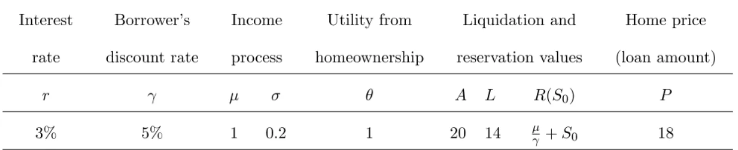
In this section we illustrate the features of the competitive FRM mortgage lending with and without re…nancing in a parametrized example. Table 1 shows the parameters of the model. The re…nancing wealth cuto¤s are set as Si K_i=11 =_f0:02i_giK₌₁1, withSK =S= 0:33.

The left-hand side of Figure 1 shows the FRM mortgage premia under a competitive lending market without re…nancing and with re…nancing allowed as a function of the borrower’s creditwor-thiness (initial wealth level). As before, no re…nancing is justi…ed by the imposition of a su¢ ciently high prepayment penalty.

Note that the borrower’s credit score increases in his wealth levelS (the likelihood of default decreases with the wealth level). The vertical lines show the wealth cuto¤s below the borrower does not qualify for a loan. We observe that mortgage premia are always decreasing in the wealth level, re‡ecting a lower likelihood of loss due to default whether or not re…nancing is allowed. The mortgage premia with re…nancing are larger compared to those without re…nancing, and more so for riskier borrowers (with lower wealth levels).

market of riskier types (those with lower wealth levels). Interestingly, it is the lender’s participation constraint that dictates the exclusion from credit. In the regime with re…nancing, the riskiest borrowers served (those with initial wealth of Sref) have a large net positive utility gain from homeownership. However, lenders cannot break even on those potential borrowers with low enough wealth, because higher mortgage premium is more than o¤set by costs associated with a higher likelihood of default.

The right-hand side of Figure 1 shows the borrower’s net utility gain from homeownership …nanced by the FRM mortgage without and with re…nancing allowed as a function of the borrower’s initial wealth level. We observe that the borrower’s net utility gain is lower when re…nancing is allowed, more so for riskier borrowers. However, a large e¢ ciency loss from re…nancing in this example comes from the exclusion of riskier types who cannot enjoy the bene…ts of homeownership. Note that one could see more high cost (high premium) loans and more defaults if prepayment penalties are used, just because more risky borrowers would be able to qualify for a loan.

6

Extensions

In this section, we discuss possible extensions of our model. We argue that, even if we take into account these additional factors, the main …nding of the model still holds: prepayment penalties do provide bene…ts to the borrowers.

This observation is based on the following argument. In order to break even, the lender has to make money on the borrowers who receive positive wealth shocks, since the lender is likely to lose money on the borrowers who receive negative wealth shocks. However, in the absence of prepayment penalties, the lender’s ability to make pro…t is more limited, since the borrowers with improved creditworthiness are able to re…nance their mortgages and get lower mortgage premia. Hence, the lender has to either charge higher mortgage premia on mortgages without prepayment penalties, or avoid serving risky borrowers at all. We maintain that the same argument is valid in

more general settings discussed below.

6.1 Stochastic House Prices

So far we have considered a time-homogeneous setting in which agents are in…nitely lived and the borrower’s average income and the liquidation and reservation values do not change over time. In a stochastic house price environment, an increase in house price would increase the borrower’s creditworthiness (due to an increase in the value of collateral and his total wealth) and thus provide an additional incentive to re…nance if this option is allowed. Similarly a decline in house price would lower the borrower’s creditworthiness and could lead to a strategic default: the borrower may default even when he is still able to make mortgage payments.

It is important to note that some of the borrowers could also re…nance to cash out part of their home equity following an increase in home value, not just to get a lower mortgage rate. However, as such re…nancings are also induced by positive credit shocks, a freely prepayble mortgage would still have the undesirable feature we identi…ed: it would allow those with ex-post good credit shocks a free exit from the credit arrangement, thus limiting ability to share credit risk among borrowers.16

Overall, our argument supporting re…nancing penalties would be stronger in a stochastic house price environment due to an additional source of variation in ex-post credit quality of the borrowers. In fact, in our empirical work we will use house price shocks as a proxy for ex-post wealth shocks.

6.2 Mobility motive to prepay

The …ndings in our model are predicated on the assumption that borrowers have no reason to prepay their mortgage except to receive a lower mortgage premium. Of course, this analysis

1 6

We note that a moderate prepayment penalty could be optimal if they are sizeable utility gains for the borrowers from cashing-out their home equity. The penalty amount may be chosen to be su¢ ciently low to allow the borrowers to re…nance in order to cash-out their home equity when truly needed at a reasonable cost, but at the same time it will be su¢ ciently high to discourage some opportunistic prepayments.

ignores other likely reasons that borrowers prepay mortgages, such as lower interest rates or the sale of a house to move to another location. Such moves may take place for employment or family reasons. Either way, borrowers who are likely to move receive a countervailing bene…t of avoiding prepayment penalties that is not in our model. What would appear in our model to be an ine¢ cient prepayment might instead be an e¢ ciency enhancing move. Prepayment penalties that restrict mobility might well have a negative welfare e¤ect.17

It is straightforward to incorporate some costs of prepayment penalties due to restricted mo-bility in our model. For the highest credit quality borrowers, the bene…t of a prepayment penalty in terms of a lower rate premium is minimal. These borrowers already receive the lowest available mortgage rate, so even a small bene…t of moving is likely enough to tip them in favor of choosing a fully prepayable mortgage. Thus we would expect that the highest quality borrowers will al-most surely want to avoid prepayment penalties. By contrast, low credit quality borrowers receive the largest discounts for accepting a prepayment penalty. For these borrowers, the likelihood of mobility or its bene…ts must be high for them to choose a fully prepayable mortgage.

To illustrate this in an example, we consider the parameterization from Section 5 and assume that the expected utility gain from mobility for a given borrower is distributed uniformly on[0;2].18 Figure 2 displays a percentage of borrowers obtaining mortgages with prepayment penalties as a fraction of total mortgages originated. As we observe, as the borrowers become less creditworthy (as their initial wealth decreases) the larger is a fraction of mortgages with prepayment penalties.

6.3 Endogenous re…nancing grid

For simplicity, we assumed that re…nancing happens on the exogenously determined re…nancing grid. A more realistic assumption is that re…nancing happens whenever it improves the borrower’s

1 7

It is worth noting that …nancial institutions can mitigate the negative e¤ects of prepayment penalties on mo-bilities. For example a prepayment penalty could be applicable for re…ancings but not for house sales.

1 8

In this example, we determine the competitive mortgage rate with no prepayment penalty assuming that the borrower’s likelihood of moving out is governed by a Poisson process with the intensity equal to 0.2.

utility by a certain amount (due, for example, to some associated transactions costs). This would endogenously determine a re…nancing grid. Since our results hold for any grid, this does not change the predictions of our model. However, it generates a new prediction. Since the bene…ts of re…nancing are higher for riskier borrowers, these borrowers are going to re…nance their mortgages more often in response to positive wealth shocks. We test this prediction using house price shocks as a proxy for ex-post wealth shocks.

6.4 Limited prepayment penalties

We have considered a …xed rate mortgage with no re…nancing, which has, by de…nition, a su¢ -ciently high prepayment penalty to discourage re…nancing, and a …xed rate mortgage that has no prepayment penalty. One of the predictions of our model is that a prepayment penalty leads to an interest rate reduction. Since loans with a prepayment penalty do not prepay in equilibrium, the interest rate reduction cannot be attributed to the possibility that the borrower pays the prepay-ment penalty to the lender thus compensating him for the lower interest rate. Instead, we show that the interest rate reduction is welfare improving.

In practice, the size of the prepayment penalty can be limited and borrowers sometimes might choose to prepay their mortgages despite the presence of a prepayment penalty. It is easy to see, however, that considering a …nite, limited prepayment penalty will not change the predictions of our model. With a limited prepayment penalty, re…nancing, although possible, is going to happen less often. Moreover, even if the borrower’s creditworthiness improves su¢ ciently so that re…nancing is bene…cial, the lender will be partially compensated with the prepayment penalty. Thus, by imposing a …nite, limited prepayment penalty, the lender will be able to extend credit to some risky borrowers and lower the mortgage premia compared to loans with no re…nancing.

A moderate prepayment penalty might also result from practical trade-o¤s in a mortgage con-tract. For example, it could be chosen to allow the borrowers to move at a reasonable cost to realize

gains from mobility, but will be su¢ ciently high to discourage some opportunistic prepayments.

6.5 Adverse selection

Another potential concern with our model is the assumption that the lender accurately observes the credit quality of the borrower. That is, lenders know as much about the likelihood of a default using observable information as the borrower. We believe this assumption is reasonable given that the lender can observe income, occupation, credit history, and the loan-to-value ratio of the property. Underwriting experience allows lenders to determine the probability distribution of defaults. Lenders are also likely to be better informed than borrowers about the distribution of future house price changes.19

We also do not take into account the possibility that a menu of contracts with and without re…nancing penalties could play a role in screening borrowers based on their ex-ante knowledge concerning some relevant variables such as the likelihood of moving20. This could be relevant if borrowers were better informed than lenders about the ex-ante riskiness of their income, wealth, or the likelihood of their mobility shocks. In such an environment, the lenders would balance the potential bene…ts of screening borrowers by o¤ering them contracts with and without re…nancing penalties against the costs of decreased ability to insure borrowers.

6.6 Non competitive lending

Our results were derived in a competitive mortgage lending market with FRM contracts. We conjecture that the ine¢ ciency of re…nancing we identi…ed would also apply to other models of competition, as exclusivity would increase total ex-ante surplus there as well. The relative bargaining powers would determine a share of an additional surplus generated by the exclusive

1 9

We recognize that possibly poor underwriting standards in the mortgage industry can makes these assumptions less plausible for the 2005 to 2007 time period. This provides an additional advantage of choosing mortgages originated in June 2003 in our empirical exercise.

2 0

relationship with the lender (due to a prepayment penalty) that the borrower would receive.

6.7 Stochastic interest rate

The bene…ts of prepayment penalties we identify should also be present in a model with stochastic interest rates, as the basic intuition behind the e¢ ciency of borrowers cross-subsidizing each other to hedge against future risks will be valid there as well.21

6.8 General risk aversion

For the sake of tractability, we assumed risk-neutrality of the borrower with respect to discretionary consumption. A more general form of risk-aversion on the borrower’s side would likely strengthen our results as the risk averse borrower would value insurance against costly default, which the lenders can better provide employing re…nancing penalties.

6.9 Endogenous downpayment

We assumed a constant (zero) downpayment by the borrower. In the health and life insurance context frontloading contributions can help alleviate the problem of reclassi…cation risk.22 In the lending context the bene…cial role of frontloading through downpayment or points would be much weaker. Those who can spend a lot on points or higher downpayments are likely already good risks. Thus, as these borrowers can receive low mortgage rates, placing a large downpayment might not bene…t them a lot.23

2 1

Piskorski and Tchistyi (2010a) derive an optimal mortgage in a stochastic interest rate environment where full exclusivity (prepayment penalty) is still optimal.

2 2

See, for example, Hendel and Lizzeri (2003).

2 3_{This is an important di¤erence with health or life insurance context where the agent’s ability to frontload an}

7

Empirical Evidence

The model in the previous section makes a number of predictions that we now examine using data on recently originated …xed rate mortgages. As suggested above, we use house price changes as a proxy for ex-post credit shocks.

One real-world complication in empirically investigating the predictions of our model is that borrowers might prepay to obtain a lower mortgage rate due to lower market interest rates, rather than because of a change in credit status. Our model does not explicitly consider how the addition of interest rate shocks could impact prepayment, though as we discussed in Section 6.7, we are con…dent that all of our main predictions would still hold. In order to ensure that our empirical work is not biased by the impact of negative interest rate shocks on prepayment, we focus on mortgages originated in June 2003. During that time period, mortgage rates were at their lowest level in the period between 1988 to 2008 (see Figure 3), minimizing the potential value of the prepayment option due to market interest rate changes. By focusing on borrowers who obtained mortgages when the market rate was the lowest in decades, any observed re…nancings must be due to factors unrelated to market interest rate declines.

7.1 Empirical predictions

Below we develop predictions that are consistent with our model.

Borrowers who receive positive credit shocks are more likely to prepay their mortgages. We examine mortgages without prepayment penalties to see how likely these mortgages are to prepay in response to house price changes. Our model predicts that borrowers who receive the largest house price increases should be the most likely to prepay early.

The sensitivity of prepayment risk to a positive credit shock is larger for lower credit quality households. Our model suggests that the worst credit risk borrowers bene…t the most from positive credit shocks such as an increase in the value of their house, and thus they should be most likely

to prepay their mortgages.

The next two predictions are based on our results showing that the bene…ts from a prepayment penalty are larger for less creditworthy borrowers, as these borrowers are the ones most likely to prepay if they receive a positive credit shock.

Prepayment penalties should be most prevalent among the riskiest borrowers. The prepayment penalty has two bene…ts for less creditworthy borrowers. First, the riskiest borrowers might not be able to qualify for credit unless they accept a mortgage with a prepayment penalty. Second, those who could qualify for credit with free re…nancing obtain a mortgage rate reduction if they accept a prepayment penalty, the larger the riskier they are. On the other hand, a prepayment penalty has virtually no bene…t for the most creditworthy borrowers. Thus we would expect a higher concentration of prepayment penalties among riskier borrowers. We examine whether the distribution of prepayment penalties as a function of borrowers’creditworthiness in the data corresponds to the one implied by our model. Finally, our model also implies the following:

Borrowers choosing prepayment penalties obtain rates that are lower than they would have obtained with fully prepayable mortgages (conditional on qualifying for credit), with the largest reductions going to the riskiest borrowers.

7.2 Data Summary

Our primary data comes from LoanPerformance (LP), a subsidiary of First American CoreLogic. LP provides loan-level data on a large number of securitized mortgages. Mayer and Pence (2009) show that the LP data appear relatively representative of the universe of high-cost risky loans, with the exception that re…nancings appear to be somewhat over-represented in LP.

LP collects its data at two di¤erent times. First, LP collects data on contract terms at the time of origination. In addition, LP also collects data on whether or not the loan has paid o¤ or become delinquent from servicers throughout the life of the mortgage. We create a combined dataset that

includes both the characteristics of a loan at origination as well as its monthly payment history. Within the LP database, we consider only loans with the following characteristics:

A. Loans that were originated in June 2003

B. Fixed interest rate (we do not consider ARMs or hybrid mortgages) C. Term lengths of 15, 20 or 30 years

D. Known prepayment penalty status (some loans have missing values) E. Located in an MSA with housing price index (HPI) data

F. Collateralized by an owner-occupied 1-4 unit home

We collect HPI data from the O¢ ce of Federal Housing Enterprise Oversight. The data are reported at the MSA level and are mapped onto the LP data using a ZIP code to MSA correspon-dence. The HPI index is normalized to re‡ect real dollars. Table 1 de…nes all the variables we use in our analysis.

We consider two subsets of the LP database: prime and subprime. Prime loans are classi-…ed by the type of pool they belong to, using de…nitions that are reported by the issuer of the mortgage-backed security. Prime MBS are backed by high-quality mortgages (that is, mortgages for borrowers with relatively low loan-to value ratios and with very good credit scores), whose initial balance typically exceeds the maximum limits for participation by government-sponsored entities Fannie Mae and Freddie Mac. Subprime loans consist of mortgages belonging to pools classi…ed as subprime and having an origination FICO score less than 620.24

We focus on …xed-rate mortgages due to complications in understanding prepayment behavior for ARMs that often have teaser rates or other features that complicate the empirical analysis by giving borrowers reasons to re…nance mortgages other than changes in their creditworthiness. After all our restrictions, we are left with a sample of 9,046 subprime FRMs (of which 2,517 carry

2 4

Most lenders de…ne a borrower as subprime if the borrower’s FICO credit score is below 620 on a scale that ranges from 300 to 850. See also Keys et al. (2010).

no prepayment penalty) and 9,628 prime FRMs that carry no prepayment penalties in order to investigate the re…nancing propensity of the borrowers.25

Table 3 reports summary statistics for the securitized loans in our sample that carry no pre-payment penalties. In general, loans in prime pools are quite safe along all dimensions and have the mean origination FICO score equal to 738. Subprime loans are much riskier with an average origination FICO score equal to 574. These statistics suggest variation across multiple risk factors that complicate our analysis. Among the categories of loans, subprime loans prepay in the …rst 16 quarters at much higher rates (70%) compared to prime loans (31%).

Houses also experience quite di¤erent rates of price appreciation depending on their location. The mean quarterly real appreciation rate was 1.3 percent (about 5% annualized), re‡ecting the strong growth of house prices over our sample period. Thus we would expect relatively few defaults, as borrowers who get into …nancial trouble can respond by paying o¤ their mortgage by selling their house, often at a pro…t. However, there is wide dispersion in house price growth rates. The highest-appreciation markets experienced quarterly appreciation rates as high as 3.3% – almost 14 percent per year for more than 4 years. Slightly less than ten percent of markets saw negative real appreciation rates over this time period.

Table 5 reports summary statistics for all securitized subprime loans in our sample, whether or not these mortgages contain a prepayment penalty, and also separately for senior and junior liens. As Table 5 shows, more than 72 percent of subprime loans have a prepayment penalty.

7.3 Empirical results

The …rst two predictions of our model state that the borrowers who receive positive credit shocks are more likely to prepay their mortgages. We begin our analysis by exploring whether the changes in borrowers’ creditworthiness proxied for by changes in house prices are an important factor

2 5_{Due to the paucity of prime mortgages with prepayment penalties, we do not examine rate di¤erences for prime}

a¤ecting re…nancing behavior.

Table 4 presents regressions that explore the prediction that higher house prices spur increased prepayments, so that over time, pools of outstanding loans are disproportionately composed of mortgages in locations with below-average house price appreciation. We use a logit speci…cation with a dependent variable that equals 1 if a loan in a given category pays o¤ and zero otherwise. The independent variable of interest is the annualized rate of house price appreciation. The speci…cations include a variety of control variables that are commonly associated with loan payo¤ and risk, including the coupon rate on the mortgage, the borrower’s FICO score, cumulative loan-to-value ratio, and whether the loan was a re…nancing or cash-out re…nancing. We run separate regressions for prime and subprime loans. For ease of interpretation, coe¢ cients in all tables re‡ect marginal e¤ects of a one standard deviation change in the variable about its mean for continuous variables, or a one unit change in the case of discrete variables.

Table 4 shows that, consistent with the …rst empirical prediction of our model, borrowers in locations where house prices appreciated sharply are more likely to prepay their mortgages compared to borrowers in locations where house prices grew less quickly. The coe¢ cient on annualized house price appreciation is positive and statistically di¤erent from zero for subprime borrowers and is positive for prime borrowers.

Our second empirical prediction is that the sensitivity of prepayment risk to a positive credit shock is larger for lower credit quality household. Consistent with this prediction, we …nd that the e¤ect of house price appreciation on payo¤ is much larger (both on an absolute and relative basis) for the riskier subprime loans. As Table 4 shows for prime mortgages, a one standard deviation change in house price appreciation (1.0 percent) leads to a modest 0.6 percent increase in the payo¤ rate, an increase of about 2 percent of the mean payo¤ rate of 31%. For the riskier subprime loans, the marginal e¤ect rises to 8.3 percent, a much larger relative increase of 11.8 percent from the mean payo¤ rate of 70%. These coe¢ cients support the conventional wisdom in the mortgage

industry that house price appreciation is an economically important factor in explaining payo¤ rates for the riskiest mortgages.

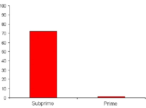
Our third empirical prediction says that the riskiest borrowers are the most likely to obtain loans with prepayment penalties. Across the two types of loans, the evidence strongly supports this prediction. As Figure 4 shows less than 2 percent of mortgages in prime pools (1.5%) have prepayment penalties, while 72.2 percent of subprime mortgages have prepayment penalties. The summary statistics of mortgages with and without prepayment penalties also show that mortgages with prepayment penalties are much riskier on observable dimensions, as measured by variables such as FICO or CLTV.

The fourth prediction of our model is that borrowers choosing prepayment penalties obtain rates that are lower than they would have obtained with fully prepayable mortgages (conditional on qualifying for credit), with larger reductions going to riskier borrowers. Empirical investigation of this prediction is challenging as we do not observe a counterfactual in the data: we do not know whether a borrower would qualify for credit for a given house without a prepayment penalty, and if so, what the corresponding mortgage rate would be. Nevertheless, to shed some light on this question, we compare the rates on loans with and without prepayment penalties, controlling for a number of observable risk characteristics. We note that our model implies that borrowers choosing prepayment penalties are likely to be less creditworthy (potentially on dimensions not captured by our set of risk controls). Thus, this potential selection on unobservables would make it harder to show that the borrowers with prepayment penalties obtain lower rates.

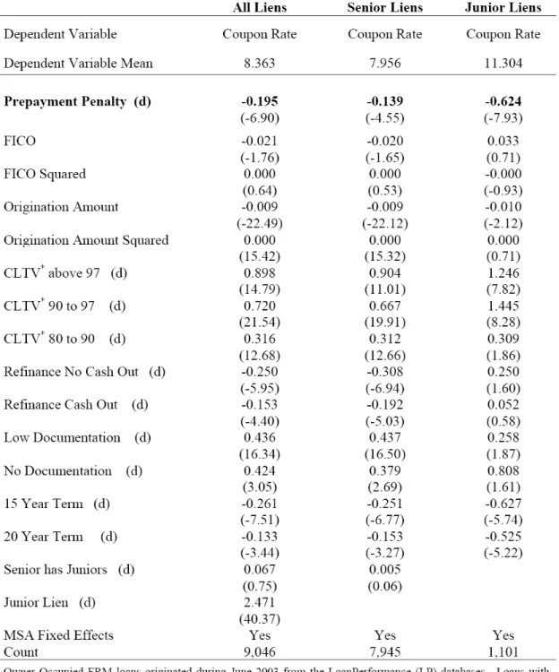
Table 6 presents the result of regressing the subprime coupon rates on the prepayment penalty status. Consistent with our model, we …nd that among risky borrowers, mortgages with pre-payment penalties carry lower rates compared with loans with free re…nancing, with the largest di¤erence for the riskiest loans. Column (1) reports results for all borrowers. The subprime bor-rowers receive mortgages with a rate that is almost 20 basis points lower (0.195 percent) when a

loan has a prepayment penalty. To further investigate this, we compare rates for borrowers for senior and junior liens. Column (2) reports the safer senior liens (the highest priority mortgages) while Column (3) presents results for riskier second liens. These junior mortgages fall behind the …rst liens in priority and have a very high average CLTV of about 100%. Thus, our model would predict larger discounts for prepayment penalties for riskier second lien borrowers than for …rst lien borrowers. Consistent with our theory, the mortgage rates of the riskiest junior liens are 62 basis points lower (0.625 percent) when their loan has a prepayment penalty, while for the …rst lien borrowers this di¤erence is 14 basis points (0.139 percent).

These di¤erences in coupon rates between loans with and without prepayment penalties are quite sizable given that the period of applicability of a typical prepayment penalty is limited. For example, among subprime loans originated in 2003, the average penalty lasted only for about three years.26

While the percentage of subprime borrowers with fully prepayable loans is relatively low (less than 30 percent), the question naturally arises as to why low credit quality borrowers would not always have prepayment penalties if the higher mortgage rates often lead to greater defaults. Our earlier discussion suggests that restricted mobility may impose additional costs that might more than o¤set the bene…t of lower mortgage rates that usually accompany a prepayment penalty. Thus, some borrowers with a high likelihood of moving might accept higher rates and a greater risk of default to compensate for avoiding being locked into their homes. In addition, in a number of states, there are legal restrictions on the usage of prepayment penalties by lenders.27

2 6

See Chomsisengphet and Pennington-Cross (2006).

8

Concluding Remarks

Critics of subprime mortgages often point to a high concentration of prepayment penalties among less creditworthy borrowers. They argue that prepayment penalties unfairly lock less creditworthy borrowers into mortgages with high interest payments.

This paper shows that in a competitive lending model, re…nancing penalties can be welfare improving, and that they can be particularly bene…cial to riskier borrowers in the form of lower mortgage rates, reduced defaults, and extension of credit. Thus, a high concentration of prepay-ment penalties among the least creditworthy borrowers can be an outcome of an e¢ cient and fair lending. Overall, our model highlights the importance of considering dynamic features of credit contracts in order to understand the impact of speci…c lending terms. We also provide some emprical evidence, which is consistent with the key predictions of our model.

Our theoretical anlysis suggests that regulations banning re…nancing penalties might have unintended consequences. Instead of protecting the riskiest would-be homeowners, the new laws might end up protecting them from credit. Our model also suggests that the re…nancing penalties could be a part of a refashioned mortgage product that helps riskier borrowers obtain credit. This might require appropriate disclosure and counseling to ensure that borrowers understand the terms of their mortgages and the implications of a prepayment penalty.

Appendix

Proof of Proposition 1

First we show that the solution to (3)-(6) is concave in S. Consider a function

F(S; ) =U S; S;

where U S; is a solution to (3)-(6). From (3)-(6) we have that

F(S; ) = + + rS+ F0(S; ) ( r)W +1 2 2_F00_{(S; )for S2 0; S}1_{( ) ;} F 0; =A; F0 S; = 0 forS S1( ); F00 S; = 0 forS S1( ):

As the solutionF is smooth we can di¤erentiate it with respect to S to obtain:

( r)F0(S; ) = rS+ F00(S; ) ( r) +1

2

2_F000_{(S; ) forS2 0; S}1_{( ) :}

Evaluating the above equation at S =S1_{( ) yields}

F000(S1( ); ) = 2( ₂ r) >0:

Note that as F00_(S1_{( ); ) = 0 and we have that F}000_(S1_{( ); ) > 0 it implies that there exists}

" > 0 such that F00 < 0 over the interval (S1( ) "; S1( )). Also as F0(S1( ); ) = 0 and F00(S1( ); ) < 0 over the interval (S1( ) "; S1( )) it implies that F0 > 0 over the interval

From (3) we have that

F00(S; ) = 2 F(S; ) [ + ( r)S] rS+ F

0_{(S; )}

2 : (20)

As and as by assumption we have that 0:Hence from (20) whenever: (i) F(S; ) <[ + ( r)S] and (ii) F0(S; ) > 0 holds it follows that F00 <0:Now since F(S1( ); ) = + ( r)S1( )and F0>0over the interval (S1( ) "; S1( ))it follows that these conditions are satis…ed over the interval (S1( ) "; S1( )). Moreover, (i) will hold for any S ₂[0; S1_{( ))as long as F remains strictly increasing, i.e. as long as F}0 _>0.

Now suppose by contradiction thatF0 0 for someS S1( ) "and let

~

S= sup S S1( ) " F0 0 :

Then it follows that F0( ~S; ) = 0; and that for all S ₂( ~S; S1( )) we have that F0 >0 and so (i) and (ii) holds. But this implies that F00<0 forS ₂( ~S; S1( )):From the Fundamental Theorem of Calculus it follows that:

S0(b)) + S1_{( )} Z ~ S F00(S; )dS;

which given thatS0(S1( ); ) = 0 implies that

F0( ~S; S1( )) = S1_{( )} Z ~ S F00(S; )dS:

As F00 <0 for S ₂( ~S; S1( )) the above implies thatF0( ~S; S1( ))> 0;which is a contradiction. Hence we have that F0 > 0 for S ₂ (0; S1( )) and hence (i) and (ii) holds and so F00 < 0 for S ₂(0; S1_{( )):But this implies thatU}0 _{S; >1 and U}00 _{S; <0forS 2( ~S; S}1_{( )):}

We note that Conditions (5)-(6) imply that

U S1( ); = + +rS1( ) (21)

The borrower’s savings (wealth) evolves according to

dSt= rSt+ dt+ dZt dCt

For an arbitrary feasible strategy (C; S), consider

Gt

Z t

0

e s(dCs+ ds) +e tU St; ; (22)

where function U satis…es all the conditions outlined in Proposition 1. We will show that Gt is a

supermartingale. Di¤erentiating (22) with respect to tand using Ito’s lemma gives

e tdGt = U St; + + rSt+ U0 St; + 0:5 2U00 St; dt

+ 1 U0 St; dCt+U0 St; dZt: (23)

When St S1( ), the …rst term in the right-hand side of (23) is zero, because of (3). When

St > S1( ), the …rst term is negative, because of (5), (6), (21) and the fact > . Since

U0 St; 1 and dCt 0,Gt is a supermartingale. E Z 0 e s(dCs+ ds) +e A = E Z 0 e s(dCs+ ds) +e S = E[G ] G0 =U S0; (24)

Thus, the agent’s payo¤ associated with strategy (C; W) is less than or equal toU S0; .

imme-diately whenever St> S1( ), thenGt is a martingale and (24) holds with equality. Hence, this is

the optimal strategy, which results in U S0; payo¤ to the agent.

Proof of Proposition 2

First we prove the following Lemma.

Lemma 3 The maximum savings level of the borrower, S1( ), is strictly increasing in the com-petitive mortgage repayment rate on the FRM with no re…nancing .

Proof Di¤erentiating equation (21) with respect to and taking into account (5) gives

@S1 @ = 1 +@U(S 1_{( ); )} @ r :

According to Feynman-Kac formula,

@U S1 _; @ = E "Z ₍S1_{( ); )} 0 e t@U St; @St dt S0=S1 # :

Since @U(_@StSt; ) 1, we can write that

@U S1 ; @ E "Z ₍S1_{( ); )} 0 e tdt # = 1 1 Ehe (S1( ); )i :

On the other hand, since S0 S1 and r < we can write that

P = V(S0; ) V(S1 ; ) = r r L E h e r (S1( ); )i < r r L E h e (S1( ); )i;

which gives E h e (S1( ); ) i r P r L : Hence, @U S1 ; @ 1 1 r P r L ! = 1 + P _r + (1 )L r L :

Noting that (Lemma 1), and as r[P (1 )L] (as by assumptionP L _r L ) we have thatP _r + (1 )L. But this implies that @U(S

1_{( ); )}

@ < 1and so

@S1_{( )}

@ >0.

Now let’s take any S0 S1( (S0)): Consider S00 < S0: Let’s suppose that by contradiction

(S₀0) < (S0). But this and Lemma 3 imply that S1 (S00) < S1 (S00) ; which implies

that (S0; (S0)) > (S00; (S00)) (as both S00 < S0 and S1 (S00) < S1 (S00) ). But this

implies that P = (S0) r E e r (S0; (S0)) (S0) r L jF0 | {z } V0(S0; (S0)) > (S 0 0) r E e r (S0 0; (S00)) (S 0 0) r L jF0 | {z } V0(S00; (S00)) ; (25)

which contradicts V0(S00; (S00)) = P: Therefore we have that the competitive mortgage rate on

FRM with no re…nancing, , is strictly decreasing on [S; S], where S is the savings level of the most creditworthy borrower. Moreover

S = inf

S SfS

1_{( (S))}

g;

as we have that d_dS(S) <0forS ₂[S; S]and @S

1_{( )}

Proof of Proposition 3

The proof of (7)-(9) is essentially the same as the proof of Proposition 1, except that the boundary condition (5)-(6) is replaced with (9).

The proof of (10)-(12) follows from the Feynman-Kac stochastic representation formula and the fact that the mortgage market value Vn(S; ) is given by

Vn(S; ) =E "Z min( ; n) 0 e rt dt+e rmin( ; n)(L+ 1 n_< (P L)) # ;

where the default and re…nancing times are

= inf_ft >0 :St= 0g;

n _{= inf}

ft >0 :St=SSn0+1g;

and the savings level evolves as follows

References

Ait-Sahalia, Yacine, Jonathan Parker, and Motohiro Yogo, 2004, Luxury goods and the equity premium, Journal of Finance 59, 2959-3004.

Campbell, John Y., and João F. Cocco, 2003, Household risk management and optimal mortgage choice,Quarterly Journal of Economics 118, 1449-1494.

Campbell, John Y., and João F. Cocco, 2007, How do house prices a¤ect consumption? Evidence from micro data,Journal of Monetary Economics 54, 591-621.

Chari, Varadarajan V., and Ravi Jagannathan, 1989, Adverse selection in a model of real estate lending, Journal of Finance 44, 499-508.

Chomsisengphet, Souphala, and Anthony Pennington-Cross, 2006, The evolution of the subprime mortgage market, Federal Reserve Bank of St. Louis Review January/February 2006.

Cocco, João F., 2004, Portfolio choice in the presence of housing, Review of Financial Studies

18, 535-567.

Cochrane, John., 1995, Time consistent health insurance, Journal of Political Economy 103, 445-473.

Demyanyk, Yuliya and Otto Van Hemert, Otto, 2008, Understanding the subprime mortgage crisis, forthcoming in theReview of Financial Studies.

Deng, Yonheng, John Quigley, and Robert Van Order, 2000, Mortgage termination, heterogeneity, and the exercise of mortgage options, Econometrica 68, 275-307.

Dunn, Kenneth B., and Chester S. Spatt, 1985, An analysis of mortgage contracting: Prepayment penalties and the due-on-sale clause,Journal of Finance 40, 293-308.