Three Essays In Commodity Price Dynamics

(1)

THREE ESSAYS IN COMMODITY PRICE DYNAMICS

AMALDABBOUS A THESIS IN THEDEPARTMENT OF ECONOMICS

PRESENTED INPARTIALFULFILLMENT OF THEREQUIREMENTS FOR THEDEGREE OFDOCTOR OF PHILOSOPHY

CONCORDIA UNIVERSITY MONTREAL´ , QUEBEC´ , CANADA

JULY2015 c

(2)

C

ONCORDIA

U

NIVERSITY

Economics

This is to certify that the thesis prepared

By: Mrs. Amal Dabbous

Entitled: Three Essays in Commodity Price Dynamics

and submitted in partial fulfillment of the requirements for the degree of

Doctor of Philosophy (Economics)

complies with the regulations of this University and meets the accepted standards with respect to originality and quality.

Signed by the final examining committee:

Chair Dr. Linda Dyer External Examiner Dr. John W. Galbraith Examiner Dr. Ian Irvine Examiner Dr. Prosper Dovonon Supervisor Dr. Bryan Campbell Approved by Dr. Effrosyni Diamantoudi Graduate Program Director

(3)

Abstract

Three Essays in Commodity Price Dynamics

Amal Dabbous, Ph.D. Concordia University, 2015

This thesis consists of three essays in commodity price dynamics. In the first essay, we embed a staggered price feature into the speculative storage model of Deaton and Laroque (1996). Interme-diate goods inventory speculators are added as an additional source of intertemporal linkage which helps us to replicate the stylized facts of the observed commodity price dynamics. The staggered pricing mechanism adopted in this paper can be viewed as a parsimonious way of approximating various types of frictions that increase the degree of persistence in the first two conditional mo-ments of commodity prices. The structural parameters of our model are estimated by simulated method of moments using actual prices for four agricultural commodities. Simulated data are then employed to assess the effects of our staggered price approach on the time series properties of commodity prices. Our results lend empirical support to the possibility of staggered prices.

The second essay investigates the determinants of the percentage change in commodity prices. We apply the dynamic Gordon growth model technique and conduct the variance decomposition for the percentage change in spot commodity prices to 6 agricultural commodities. The model ex-plains the percentage change in spot commodity prices in terms of the expected present discounted values of interest rate, yield spread, open interest and convenience yield. Empirical results indicate that the model is successful in capturing a large proportion of the variability in the 6 agricultural commodity prices. Moreover, we show that yield spread and open interest help predicting changes in commodity prices.

Finally, the third essay evaluates different hedging strategies for eleven commodities. In addi-tion to the tradiaddi-tional regression hedge ratio model (OLS) and the vector error correcaddi-tion model (VECM), we estimate dynamic hedge ratios using the conventional dynamic conditional correla-tion model (DCC) of Engle (2002) and the diagonal BEKK model (DBEKK) of Engle and Kroner (1995). Moreover, we propose two more advanced models, the DCC model and the DBEKK

(4)

model that will account for the impact of the growth rate of open interest on market’s volatility and co-movements of commodity spot and futures returns. The empirical analysis shows that adding the growth rate of open interest improves the in-sample hedging effectiveness of the DCC model. Furthermore, the out-of-sample hedging exercise empirical results show that static models present the best out-of-sample hedging performance for 5 of the commodities. The DCC model presents the smallest basis variance for 4 of the commodities. The DBEKK model with the growth rate of open interest performs the best in terms of the basis variance reduction for corn and wheat. Our out-of-sample empirical findings provide important implications for futures hedging and highlight the fact that the use of static models to determine the optimal hedge ratio could be more effective than the use of dynamic hedge ratio models.

(5)

Acknowledgments

I would like to express my sincere gratitude to my supervisor Prof. Bryan Campbell for his con-tinuous support, patience, motivation and immense knowledge. Prof. Campbell was abundantly helpful and offered invaluable assistance, insightful comments and guidance. Moreover, I would like to thank him for giving me the opportunity to present the first essay of this thesis at CIRANO1, and helping to complete some empirical works of this part there.

I would also like to convey thanks to my then supervisor Prof. Nikolay Gospodinov and my colleague Dr. Hirbod Assa for collaborating on the first chapter of the thesis, which is a joint work with them.

Deepest gratitude are also due to the member of the supervisory committee. In particular, I would like to thank Prof. Dovonon and Prof. Irvine for their support during my studies at Con-cordia. I would also use this occasion to convey my thanks for Prof. LeBlanc (the economics department chairperson) and to Prof. Diamantoudi (the graduate program director) for their con-tinuous help and guidance.

Last but not the least I would like to express my love and gratitude to my beloved family, particularly my husband (Zaher), my kids (Ziad and Mazen), my mother and my twin sister (Imane) for their understanding and endless support and patience, through the duration of my studies.

(6)

List of Figures

1.1 Actual and Simulated Data for Soybeans Prices . . . 28

1.2 Impulse Response Function Based on Simulated Data for Soybean Prices . . . 29

1.3 Distribution of ˆβ . . . 30

1.4 Distribution of ˆα . . . 31

2.1 Actual and Forecasted Percentage Change in Price: BO . . . 56

2.2 Actual and Forecasted Percentage Change in Price: C . . . 56

2.3 Actual and Forecasted Percentage Change in Price: CT . . . 57

2.4 Actual and Forecasted Percentage Change in Price: O . . . 57

2.5 Actual and Forecasted Percentage Change in Price: S . . . 58

2.6 Actual and Forecasted Percentage Change in Price:W . . . 58

3.1 In-Sample Hedge Ratios for BO, C, CT and O for OLS, DCC and DCCoi Models . 97 3.2 In-Sample Hedge Ratios for S, W, KC and GC for OLS, DCC and DCCoi Models . 98 3.3 In-Sample Hedge Ratios for CC, SB and FC for OLS, DCC and DCCoi Models . . 99

3.4 Out-of-Sample Hedge Ratios for C and W . . . 100

3.5 Out-of-Sample Hedge Ratios for GC and CC . . . 101

3.6 Out-of-Sample Hedge Ratios for O, CT and KC . . . 102

(9)

List of Tables

1.1 Parameter Estimates from the DL Model . . . 23

1.2 First-Order Autocorrelations for the DL and ADG Models . . . 24

1.3 First-Order Autocorrelations for the Ng and Ruge-Murcia (2000) and ADG models 25 1.4 Description of Commodity Price Data . . . 26

1.5 Parameter Estimations of the ADG Model Using SMM . . . 26

1.6 First-Order Autocorrelations for Simulated Price Series . . . 27

1.7 First-Order Autocorrelation, andβ andα Parameters from a GARCH(1,1) Model . 27 2.1 Trading Characteristics of Commodity Prices Data . . . 51

2.2 Autocorrelation for the Variables Included in the Model . . . 51

2.3 Autocorrelation for the Percentage Change of the Variables Included in the Model . 52 2.4 Standard Deviations for the Variables Included in the Model . . . 52

2.5 Skewness for the Variables Included in the Model . . . 53

2.6 Excess Kurtosis for the Variables Included in the Model . . . 53

2.7 Data Statistics for the Common Variables . . . 53

2.8 Actual and Estimated Variance of the Percentage Change in Commodity Prices . . 54

2.9 Variance Decomposition of the Percentage Change in Spot Price: Variances Shares 54 2.10 Variance Decomposition of the Percentage Change in Spot Price: Covariances Shares 55 3.1 Trading Characteristics of Commodity Prices Data Obtained form CRB . . . 84

3.2 Trading Characteristics of Commodity Prices Data Retrieved from Bloomberg . . . 84

3.3 Johansen MLE Estimates, Trace statistic . . . 85

3.4 Johansen MLE Estimates, Maximum Eigenvalue Statistic . . . 85

3.5 Parameter Estimates of the VECM Model of the Mean Equations . . . 86

(10)

3.7 Future Variance Returns Equation Parameters and t-test Values of the DCC Model . 87 3.8 Spot Variance Returns Equation Parameters and t-test Values of the DCCoi Model . 88 3.9 Future Variance Returns Equation Parameters and t-test Values of the DCCoi Model 89

3.10 Correlation Equation parameters and t-test Values of the DCC Model . . . 90

3.11 Correlation Equation Parameters and t-test Values of the DCCoi Model . . . 90

3.12 Parameter Estimates of the DBEKK Model, CRB Data . . . 91

3.13 Parameter Estimates of the DBEKK Model, Bloomberg Data . . . 91

3.14 Parameter Estimates of the DBEKKoi model, CRB Data . . . 92

3.15 Parameter Estimates of the DBEKKoi Model, Bloomberg Data . . . 92

3.16 In-Sample Hedge Ratio Estimates of the DCC and the DCCoi Models . . . 93

3.17 In-Sample Hedging Effectiveness of the DCC and the DCCoi Models . . . 93

3.18 In-Sample Hedge Ratio Estimates of the DBEKK and the DBEKKoi Models . . . . 94

3.19 In-Sample Hedging Effectiveness of the DBEKK and the DBEKKoi Models . . . . 94

3.20 Comparing Out-of-Sample Basis Variance . . . 95

3.21 Ranking the Models in Terms of Basis Variance Reduction . . . 95

3.22 Comparing Out-of-Sample Basis Variance for OLS, Best Performing Model and Extreme Cases Hedge Ratios . . . 96

(11)

Chapter 1 A Staggered Pricing Approach to Modeling

Speculative Storage: Implications for

Commodity Price Dynamics

1.1 Introduction

The last decade has witnessed a surge in commodity prices and a widespread financialization of commodity products. The upward movements and the increased volatility of the commodity prices have been largely attributed to strong demand by China and other emerging markets as well as massive capital flows into the commodity markets by institutional investors, portfolio managers and speculators. While the importance of commodity price movements for the economic policy and investors’ sentiment has generated a substantial research interest, the behavior and the deter-mination of commodity prices is not yet fully understood. The main objective of this chapter is to develop a structural model of commodity price determination that reflects the empirical properties (high persistence and conditional heteroskedasticity) of commodity prices. In order to achieve this goal and to gain further understanding into the fundamental factors that drive the observed behav-ior of commodity prices, we modify the structure of the speculative storage model from one where the prices adjust almost instantaneously to harvest shocks to a setup where they change slowly and infrequently. More specifically, we depart from the assumption that market prices are determined in a perfectly competitive environment and extend the basic speculative storage model by explicitly

(12)

introducing intermediate goods speculators with a staggered pricing rule. One appealing aspect of this approach is its ability to mimic some important characteristics of the actual commodity prices such as high persistence and conditional heteroskedasticity, which can be generated even in the absence of correlated harvest shocks.

The speculative storage model for commodity prices can be dated back to Gustafson (1958) who defines a set of optimal storage rules that state how much grain should be carried over into the next period given the current year supply. Moreover, by introducing intertemporal storage arbitrage and supply shocks, Gustafson (1958) incorporates rational expectations. This line of research is further elaborated in Muth (1961). Samuelson (1971) develops a model for commodities which de-termines the behavior of the prices as the solution to a stochastic dynamic programming problem. Furthermore, Beck (1993) builds upon the work by Muth (1961) and provides a theoretical basis for treating the variance of storable commodities as serially correlated which suggests that com-modity prices may exhibit conditional heteroskedasticity. The presence of storage is instrumental in ensuring that the price variance in one period directly affects inventory variance which in turn is transmitted to next period’s price variation. Williams and Wright (1991) provide a comprehensive discussion of the basic storage model and its extensions and summarize the time series properties of storable commodities. Williams and Wright (1991) put an emphasis on the complex non-linear storage behavior resulting from the fact that aggregate storage cannot be negative.

Deaton and Laroque (1992, 1995, 1996) develop a partial equilibrium structural model of com-modity price determination and apply numerical methods to test and estimate the model parame-ters, confronting for the first time the storage model with the documented behavior of actual prices. Their analysis suggests that the introduction of speculative inventories and serially correlated sup-ply shocks do not appear to generate sufficient persistence in commodity prices although they prove to be successful in replicating the substantial volatility observed in the actual data.

More recently, numerous studies have focused on modifying the storage model in order to accommodate the persistence of commodity prices. Chambers and Bailey (1996) relax theiid as-sumption on harvest shocks, and study the price fluctuations of storable commodities, assuming that shocks are either time dependent or that the model exhibits periodic disturbances. Ng and Ruge-Murcia (2000) incorporate additional features into the storage model in an attempt to gener-ate a higher degree of persistence in commodity prices. In particular, Ng and Ruge-Murcia (2000) allow for serially correlated shocks assuming that harvest follows a first-order moving average

(13)

(MA(1)) process. They also examine the ability of production lags and heteroskedastic supply shocks, multi-period forward contracts and convenience yields to generate an increased persis-tence in commodity prices. Cafiero, Bobenrieth, Bobenrieth, and Wright (2011) demonstrate that the competitive storage model can give rise to high levels of serial correlation observed in com-modity prices if more precise numerical methods are employed. Moreover, estimates for seven commodities supported the specification of the speculative storage model with positive constant marginal costs and no deterioration, which is in line with Gustafson (1958).

Furthermore, Cafiero, Bobenrieth, Bobenrieth, and Wright (2011) use a maximum likelihood framework to estimate the storage model with stock-outs, which is extended to include unbounded harvests and free disposal. Their results produce more accurate small sample estimates of the struc-tural parameters of the model compared to the previous studies based on the pseudo-maximum likelihood procedure. Miao and Funke (2011) add shocks to the trends of output and demand. Evans and Guthrie (2007) include transaction cost frictions into the speculative storage model. One important finding that emerges from their analysis is that these frictions tend to have ex-planatory power for the dynamic behavior of spot and futures commodity prices. In a competitive equilibrium framework, the model of Evans and Guthrie (2007) is able to capture the serial cor-relation and GARCH characteristics of commodity prices. Finally, Arseneau and Leduc (2012) embed the speculative storage model into a general equilibrium framework. Their main result is that the interaction between storage and interest rates in general equilibrium increases the impact of competitive storage on commodity prices and leads to higher persistence than the one observed in the storage model with fixed interest rate.

In spite of this extensive literature for understanding the determinants and the dynamic patterns of commodity prices, reproducing the documented high persistence and conditional heteroskedas-ticity of actual prices within a well-articulated structural model proved to be a challenging task. In this chapter, we address the issues regarding the commodity price dynamics in a unified fashion by embedding a staggered pricing mechanism into the speculative storage model. While Arseneau and Leduc (2012) also suggest to “introduce staggered price setting on the part of the final goods producing firm” in a general equilibrium framework as a possible extension for future research, our work is the first to implement this approach and assess the properties of the model-generated commodity prices against the observed data.

(14)

storage activity, Newbery (1984), Williams and Wright (1991), and McLaren (1999) investigate the effects of market power on the storage behavior. Our model differs from their work along the dimension that the final bundler does not store the good and the storage is only done by interme-diate risk neutral speculators. The final bundler only bundles intermeinterme-diate prices in order to set the final price. Moreover, Rust and Hall (2003a) present a model of optimal price speculation by a middleman in the steel market. A third player, the middleman is added endogenously to the model. The middlemen will purchase steel from producers and other middlemen in the market and sell it at a mark up to retail consumers in order to make profits. The firm makes a purchase only when the current level of inventory is below a purchase threshold. The authors use the simulated minimum distance estimator to estimate the structural parameters of the model since wholesale prices are endogenously sampled, that is, wholesale prices are only observable on the dates when the middleman purchases steel.

In addition, Rust and Hall (2003b) introduce a model in which producers and consumers in the steel market can choose between two intermediate market players, a market maker which typically owns or is member of a centralized exchange where bid and ask prices are publicly known, and a middlemen. In their model, the share of trade intermediated by middleman and market makers are endogenously determined. In the steel market there are no market makers, traders have to search and bargain to find the lowest price. They show that it is possible for those two intermediaries to coexist in the market. They discuss first a market equilibrium in which only middlemen exist assuming there is a continuum of middlemen. Furthermore, they define conditions under which the presence of a single market maker or monopolist is possible with the presence of middlemen, even though surviving middlemen tend to reduce their bid and ask spreads to undercut the market maker prices. They also present the range of equilibrium outcomes when the market has four players: consumers, middlemen, market maker and producers. Finally, Mitraille and Thille (2009) examine the market power in production with competitive storage by analyzing the effects that competitive storage has on the behavior of a monopolist. Using his market power, the monopolist can influence speculative activity by manipulating prices and consequently affect the distribution of prices. One of the findings of Mitraille and Thille (2009) is that stockouts occur less frequently under monopoly.

The focus of this chapter is on the improved ability of the storage model with staggered prices to account for the empirical features of commodity prices. The main impact of staggered prices

(15)

in our model is to dampen the movements in prices as well as the market power of intermediate speculators to affect prices. This leads to gradual adjustments and persistent responses of prices following a harvest shock. In addition to generating sufficient persistence in commodity prices, the staggered pricing approach allows us to match other important moments in the unconditional and conditional distributions of the commodity prices.

Nominal price rigidity is often incorporated in dynamic general equilibrium models with two widely used nominal price rigidity specifications in the literature. On one hand, the partial adjust-ment model developed by Calvo (1983), Rotemberg (1987), and Rotemberg (1996) allows for only a randomly chosen fraction of firms to adjust their prices according to some constant hazard rate in any given period. On the other hand, the staggered price setting rule adopted by Taylor (1980) and Blanchard and Fisher (1989) permits all firms to optimize their prices after a fixed number of periods.

In this chapter, we assume that the pricing decisions are staggered as in Calvo (1983) and use a similar modeling framework as the one developed in McCandless (2008). Even though the staggered pricing is not generated endogenously within the model, it serves as a useful device to impart the inefficiencies in the agricultural commodity markets such as price floors, subsidies, import/export quotas and controls, government strategic stock reserves, collusion etc. that prevent prices to adjust instantaneously to changes in economic conditions. Note that these types of market inefficiencies allow us to depart from the typical assumption in the literature that commodities tend to be homogeneous products whose prices are fully flexible and equal to their marginal costs. Our results confirm the importance of staggered prices for commodity price dynamics and suggest that the staggered pricing mechanism appears to be consistent with the behavior of the actual data. Moreover, we show how our model can be used to analyze the response of commodity prices to harvest shocks which provides a framework for economic and policy evaluation.

The remainder of the chapter is organized as follows. The competitive storage model with staggered prices as well as the statistical characterizations of this model are presented in Section 2. Section 3 studies the practical implications of our staggered price speculative storage model using simulated data. Section 4 contains a brief description of the data and the estimation method used in the paper, and presents the main empirical results. Section 5 concludes.

(16)

1.2 Competitive Storage Model with Staggered Prices

This section introduces the model setup and characterizes the equilibrium and statistical behavior of the model-generated commodity prices.

1.2.1 Model and Equilibrium Price Behavior

The rational expectations model determines the optimal inventory decisions by risk- neutral spec-ulators. The basic version of the model developed by Deaton and Laroque (1992, 1995, 1996)1 incorporates competitive storage into the consumer demand and supply dynamics and establishes the concept of stationary rational expectations equilibrium (SREE). The model with serial correla-tion in harvest shocks is tested by Ng and Ruge-Murcia (2000). In their paper, Ng and Ruge-Murcia (2000) consider an MA(1) specification for the model harvest shocks. Our model complements and extends the original DL model by embedding a staggered price setting into the speculative storage model. Regarding the harvest shock specification, we consider both (i)iidharvest shocks and (ii) MA(1) harvests shocks.

Our modified model has three types of commodity market participants: final consumers, inter-mediate risk neutral speculators and a bundler2 who bundles the commodities in order to set the final price. In the absence of storage, the behavior of final consumers is characterized by a linear inverse demand function

pt=P(zt) =a+bzt,

whereaandb<0 are parameters to be estimated andz_t denotes the harvest in periodt. Let the harvestz_t be given by

zt =z¯+ut,

where ¯z is constant (perfectly inelastic) and u_t is a random disturbance term which is assumed either to beiid or to follow an MA(1) process

u_t =e_t+ρet−1,

1_{For brevity, we denote hereafter the basic speculative storage model of Deaton and Laroque by DL.}

2_{In the literature, it is common to use the term “monopolist” instead of the term “bundler” that we use in this} chapter. The reason that we prefer the latter is the following: in the staggered pricing literature, the final goods producer maximizes profits by setting the price. In this chapter, we do not consider any profit maximization and any type of price setting for the final goods producer. Instead, we use directly the final goods prices as set in (1.6).

(17)

wheree_tisiid(0,σ2). Ifρ=0,we have the case ofiidshocks as in DL, and whenρ>0,we have MA(1) shocks as in Ng and Ruge-Murcia (2000). In this chapter, we investigate both cases and show that when we add staggered prices, the case for ρ=0 gives better results compared to the case of non-staggered prices andρ>0.

Intermediate risk neutral speculators or inventory holders know the current year harvest and demand the commodity to transfer to the next period. They will do so whenever they expect to make a profit above the storage and interest cost. The depreciation rate of storage is denoted by δ. A simple form of proportional deterioration is considered which means that if in periodt the speculators store I units of the commodity, they have at their disposal (1−δ)I units at the beginning of the next period. Moreover, speculators have to pay the real interest rate on the value of their storage. Let rdenotes the constant exogenous real interest rate. The sum of harvest and inherited inventories, denoted byx_t,is referred to as the amount on hand and is given by

xt= (1−δ)It−1+zt.

The relationship between the amount of storage and its net profit can be summarized as

(

I_t>0 if(1−δ)/(1+r)_Et[pt+1] =pt,

It=0 otherwise,

where_Et denotes the expectation given the information at timet.

The condition for non-negative inventories is the crucial source of non-linearity in the model. This specification does not allow the market participants to borrow commodities that have not yet been grown. In addition, intermediate speculators benefit from market power that reflects their ability to affect the price. In this framework, we assume that there is a continuum of intermediate speculators (of unit mass indexed byk∈[0,1]) and final big players in the market. Final players collect all the commodities from intermediate speculators and bundle intermediate speculators’ prices into the final price in order to sell the commodity to consumers.

For simplicity, we assume that there exists a bundler who bundles all intermediate speculators’ prices into a single one. Each period t, a fraction 1−γ (0<1−γ <1) of the speculators is able to exploit their market power and to reset the prices of their commoditiesP_t∗(k). In contrast, those who did not benefit from their market power to affect prices, retain their last period prices:

(18)

P_t∗(k) =P_t−∗₁(k). Given this staggered pricing rule, along with the assumptions that speculators are risk neutral and have rational expectations, intermediate speculators’ current and expected future prices must satisfy

P_t∗(k) =max p(x_t),(1−γ)1−δ 1+rEt[P ∗ t+1(k)] +γPt∗(k) . (1.1)

The first term in the brackets represents the price if the harvest is sold to consumers in periodtand no inventories are carried over to the next period. The second term is known as the intertemporal Euler equation. This is the value of one unit stored if 1−γ of the speculators benefit form their market power to affect the price. This, in turn, occurs if the speculators expect to cover their costs (after depreciation) from buying the commodity at timet. Since the current period bundler prices are not yet determined, it is important to stress that speculators, who do not reset their prices, use their own current prices and not the market ones in order to determineP_t∗(k)in (1.1).

Finally, the bundler will bundle all intermediate prices together according to the following pricing rule (see McCandless (2008))

P_t1−ψ =γP_t−1−₁ψ+ (1−γ)P_t∗(k)1−ψ,

wherePt denotes the bundler final price of the good, the parameterψ is the gross markup of the intermediate goods speculators andP_t∗(k)represents the price for intermediate goods speculators who can set their prices. Since all intermediate goods speculators who can fix their prices are assumed to have the same markup over the same marginal costs, P_t∗(k) is the same for all inter-mediate risk neutral speculators who adjust their prices. Prices for interinter-mediate speculators who cannot set their prices are the same as the previous period prices denoted byP_t−₁.

In order to simplify the bundler’s pricing rule, we use the log-linearized version of this equation so that the final price becomes

˜

p_t =γp˜t−1+ (1−γ)p˜∗t(k), (1.2) where ˜pt and ˜p∗t denote the logarithm ofPt andPt∗, respectively.

It is worth noting that our model bears some resemblance with the model introduced in Rust and Hall (2003a) and Rust and Hall (2003b), the idea of introducing intermediate risk neutral specula-tors and a bundler is very similar to middlemen and market maker introduced in their steel market

(19)

model. As in their model, we also assume that there is a continuum of intermediate risk neutral speculators whose prices are not publicly known and that benefit from market power to affect the price and a bundler that will decide the final price at which the commodity is sold to consumers. Moreover, the final bundler price in our model is known and available to final consumers, which is similar to the market maker price in Rust and Hall (2003b) paper. However, the major difference resides in the fact that we add the staggered pricing rule exogenously to model intermediate risk neutral speculators ’ prices, whereas wholesale prices in the steel market model are endogenously sampled.

After completing the description of our model, we elaborate on some important implications of equation (1.1). As implied by this equation, the intermediate risk neutral speculators’ price follows a non-linear first-order Markov process with a kink at the price above which we do not have inventories. In the case ofiidshocks, the kink is determined by

ˆ

p= (1−γ)1−δ

1+rEp(z) +γpˆ.

This implies that

ˆ

p= 1−δ

1+rEp(z), (1.3)

which coincides with the kink given in DL.

However, as in Chambers and Bailey (1996), the price kink ˆpin the case of correlated harvests shocks is no longer constant and varies with the current harvest. This is due to the fact that with serially correlated harvest shocks, speculators form their price forecasts using all the information contained in the current shock.

Under some regularity conditions, most notably r+δ >0 and that z has a compact support, DL establish the existence of a solution to (1.1) whenγ =0 and shocks are independent. Indeed, to show the existence of the demand function for non-independent shocks, it is enough to prove the independent case conditioning on timet. In our case, we proceed by following a similar approach to proving that such an equilibrium exists. Assume that the demand x_t always lies in a subset

(20)

Definition Assume that γ ∈[0,1). A staggered stationary rational expectation equilibrium (SS-REE) is a price function f :_X×_Z→_Rwhich satisfies the following equation

p_t= f(x_t,z_t) =max p(x_t),(1−γ)1−δ 1+rEtf(zt+1+ (1−δ)It,zt+1) +γf(xt,zt) , where , I_t=x_t−p−1(p_t) =x_t−p−1(f(x_t,z_t)). (1.4) This defines the price function

P_t∗(k) = f(xt,zt),

where f(xt,zt)is the unique, monotone decreasing in its first argument, solution to the functional equation. Since this price function is non-linear, numerical techniques similar to the ones adopted by DL and Michaelides and Ng (2000) are used to solve for f(x_t,z_t)

f(x_t,z_t) =max p(x_t),(1−γ)1−δ 1+rEtf((zt+1+ (1−δ)It),zt+1) +γf(xt,zt) .

In the case of independent shocks, we can remove the time subscript and the shocks in f.

When γ =0 and the shocks are iid, we have the same model as the one considered by DL. Hence, the equilibrium is simply called SREE. In the following theorem we show that the stag-gered stationary rational expectation equilibrium (SSREE) coincides with the stationary rational expectation equilibrium (SREE) derived from the basic DL speculative storage model.

Theorem 1.2.1 If shocks are iid, then SSREE=SREE.

Proof See Appendix A.

Remark Theorem 1.2.1 shows thatp_t=P_t∗. This allows us to use all of the results for the process

p_t, that are available in the literature, for the processP_t∗.

We next show that the final demand for the bundler in our staggered speculative model is differ-ent form the one in DL. It proves useful to compare the price processes in the speculative storage model with and without staggered prices for the market participants who can reset their prices. In the basic speculative storage model of DL, the market participants cannot hold negative invento-ries. If prices are expected to increase or decrease by less than the cost of carrying the commodity

(21)

from one period to another, inventories are zero. If inventories are positive, the expected price next period is equal to the current price plus the storage costs. The final price of the commodity in the basic speculative storage model satisfies

p_t=max p(x_t),1−δ 1+rEtpt+1 . Hence, ( p_t= 1−δ 1+rEtpt+1 ifIt>0; p_t=p(x_t) ifI_t=0.

However, as stated in the description of our speculative storage model with staggered prices, the intermediate risk neutral speculators price function satisfies

P_t∗=max p(xt),(1−γ)1−δ 1+rEtP ∗ t+1+γPt∗ . In this case, ( P_t∗= (1−γ)1₁−_+rδ_EtPt+∗ 1+γPt∗, ifIt >0; P_t∗= p(xt) ifIt =0. (1.5)

It can be easily seen from (1.5) that the prices for intermediate risk neutral speculators who can adjust them satisfy the same equation as the one that speculators face in the basic storage model of DL.

Since the final price process in the speculative storage model with staggered prices is given by

˜

p_t =γp˜t−1+ (1−γ)p˜∗t(k), (1.6) one can infer that the demand of the bundler (the final demand) will be different from the demand presented by DL in the basic speculative storage model. We expect the final demand for speculative storage model with staggered prices to be in between the DL demand and the regular market demand. Moreover, we expect this demand to be more inelastic than the one derived from the basic speculative storage model. This is more consistent with the commodity elasticities estimated from actual data.

(22)

1.2.2 Statistical Characterization

Under the assumption of iid harvests shocks, the final log-price process satisfies equation (1.6). The bundler price can then be written as

P_t =P_t−₁γ _P∗

t

1−γ

. (1.7)

The persistence of commodity prices is then simply an outcome of the staggered prices which is extensively discussed in the literature on staggered pricing. Here, we provide an alternative explanation. From the logarithmic form of the relation (1.7), we have by induction that

˜ pt+1= (1−γ) t

∑

i=0 γip˜_t+∗ ₁_−i which in turn yields

P_t+₁= t

∏

i=0 P_t+∗ ₁_−iγi !1−γ .

This shows thatPt+1shares overlapping terms prices in previous periods which gives rise to high

persistence.

Next, we show that the final prices of the bundler exhibit conditional heteroskedasticity which is another salient characteristic of the observed commodity prices. Note that from (1.7), we have

Et−1(Pt2) =Pt−12γEt−1(Pt∗ 2(1−γ)₎ (1.8) and (_Et−1Pt)2=Pt−12γ(Et−1(Pt∗ 1−γ ))2. (1.9)

Combining (1.8) and (1.9) and assuming that the shocks are iid, the conditional variance of the final prices is given by

Vart−1(Pt) =Pt−12γ h E f(z+ (1−δ)It−1)2(1−γ) −(_E(f(z+ (1−δ)It−1)1−γ)2 i . (1.10)

(23)

In the absence of inventories in the previous period,I_t−₁=0, the variance reduces to Vart−1(Pt) =Pt−12γVar f(z)1−γ

. (1.11)

From (1.10) and (1.11), we can see that the variance is time-varying and, as a result, the final commodity prices derived from our model exhibit conditional heteroskedasticity. In addition, it is worth noting that the variance also depends on the value ofγ.

It is interesting to point out that the form of the conditional variance in (1.11) bears strong re-semblance to modeling the conditional heteroskedasticity in interest rate models (see, for instance, Brenner, Harjes, and Kroner (1996)). In these models, there is a parameter that allows the volatility of interest rates to depend on the level of the process. Similarly, higher values of the parameter γ in equation (1.11) indicate that the volatility of commodity prices is more sensitive to their past level which generates volatility clustering.

1.3 Model Comparisons Using Simulated Data

In this section we examine the statistical properties of the simulated data from our commodity price model with staggered pricing. In order to assess the qualitative and quantitative implications of our model, we compare it to the basic speculative storage model of DL and the modified version of the speculative model of Ng and Ruge-Murcia (2000). The model of Ng and Ruge-Murcia (2000) extends the DL model by adding serially correlated harvest shocks that follow an MA(1) process, as well as gestation lags, heteroskedastic supply shocks, multi-period forward contracts and convenience yields.

In our simulations, we calibrate the models using the parameter values estimated by Deaton and Laroque (1996) for a set of 12 commodities. These parameters (a,b,δ), presented in Table 1.1, are the same as the parameters used by Ng and Ruge-Murcia (2000). The data are simulated usingiid

harvest shocks or MA(1) harvest shocks with an MA parameterρ=0.8. We denote our speculative storage model with staggered prices by ADG.

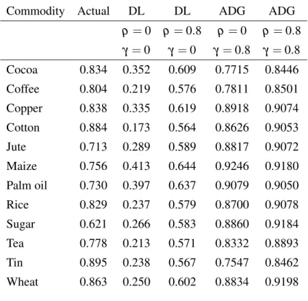
Table 1.2 presents the results for the first-order autocorrelation of the simulated prices from the different models. The first column of Table 1.2 reports the autocorrelations from the actual data used in Deaton and Laroque (1996), the second column shows the results from the basic DL model

(24)

(ρ =0) and the third column contains the results obtained using DL model with MA(1) shocks (ρ =0.8). The highest autocorrelation for the simulated prices from the DL model is for Maize (0.413 for the basic DL model and 0.644 for the specification with MA(1) harvest shocks). For all other commodities, the serial correlation in the simulated prices is well below the persistence in the actual prices.

The last two columns of Table 1.2 report the results from our model. For all commodities, the autocorrelation coefficients of the simulated prices based on the ADG model are much higher than those of the DL model specifications and are very close to the autocorrelations obtained from actual data. Once we account for staggered pricing, the additional effect of serially correlated harvest shocks is minimal.

Furthermore, Table 1.3 lends additional support to our ADG model with staggered prices. In this table, we compare the autocorrelation coefficients for the model by Ng and Ruge-Murcia (2000) with gestation lags, overlapping contracts and convenience yields to those computed from our ADG model in columns 4 and 5 of Table 1.2.

Ng and Ruge-Murcia (2000) add gestations lags to the DL basic specification in an attempt to reduce the number of periods where the intertemporal price link between periods with and without production is severed. Consequently, this increases the serial correlation in prices. For this purpose, Ng and Ruge-Murcia (2000) assume that there are odd and even periods and that harvest takes place in the even periods. Hence, the random disturbance term of the harvest process has a variance that could differ if the period is odd(σ1)or even(σ2). The highest autocorrelations are reached for a

value of σ2

σ1 =1.8. This model is denoted by GL. The results from the GL specification are reported

in column 2 of Table 1.3.

Ng and Ruge-Murcia (2000) also show, in contrast to the earlier literature on storage where contracts are absent and stockholders are free to roll-over their inventories, that a model with overlapping contracts can partially explain the high serial correlation in prices. Column 3, denoted by OV in Table 1.3 reports the corresponding autocorrelation coefficients.

Finally, Ng and Ruge-Murcia (2000) add a convenience yield to the DL model. Since inventory holders might derive convenience from holding inventories, Ng and Ruge-Murcia (2000) introduce both a speculative and a convenience motive for inventory holding. Hence, since the convenience yield partially compensates inventory holders for the expected loss when the basis is below carrying charges, their model with convenience yield generates a smaller number of stock-outs and, as

(25)

a result, the demand for inventories for convenience purposes strengthens the intertemporal link resulting in a higher persistence of prices. Results forc=50 are reported in column 4 of Table 1.3. The model is denoted by CY.

Overall, the results in Table 1.3 suggest that the different specifications of Ng and Ruge-Murcia (2000) cannot generate autocorrelation coefficients greater than 0.640 and they are below the au-tocorrelation coefficients from our ADG model and the actual data across all commodities.

1.4 Empirical Application

This section presents new empirical results from estimating the structural parameters of our pro-posed model using monthly data for four agricultural commodities.

1.4.1 Data

The data set employed in this empirical application consists of prices for four agricultural com-modities: sugar, soybeans, soybean oil and wheat. The commodity prices are obtained from the Commodity Research Bureau and are available at daily frequency for the period March 1983 – July 2008. The trading characteristics of these commodities are summarized in Table 1.4.

The spot price is approximated by the price of the nearest futures contract. Monthly commod-ity price series are constructed from daily data by averaging the daily prices in the corresponding month. The monthly frequency is convenient for studying the persistence and conditional het-eroskedasticity in commodity prices. The real commodity prices are obtained by deflating the nominal spot prices by the CPI (seasonally adjusted) index obtained from the Bureau of Labor Statistics (BLS). Each deflated price series is then further normalized by dividing by the sample average. By performing this additional normalization, each series has a historical mean of one which allows us to conduct easier comparisons of the estimated parameters across various price series.

1.4.2 Estimation Method: Simulated Method of Moments

This section provides a brief description of the simulated method of moments (SMM) which is used for estimating the model parameters. The main advantage of SMM lies in its flexibility of

(26)

the choice of moment conditions that allow us to identify the staggered pricing parameterγ. See Pakes and Pollard (1989), Lee and Ingram (1991) and Duffie and Singleton (1993) for a detailed description of the method and its asymptotic properties, and Michaelides and Ng (2000) for an investigation of its finite-sample properties in the context of the speculative storage model.

The SMM estimator requires repeatedly solving the model for given values of the structural parameters. For this reason, we present some computational details regarding the solution of the model. The function f(x) is approximated using cubic splines and 100 grid of points for

x. This function is calculated using an iterative procedure, starting with an initial value f₀(x) =

max[p(xt),0]. As in DL, the interest rateris not estimated but it is fixed at 5 percent per annum or 0.41 percent(r=1.05121 −1=0.0041)per month. In addition, we calibrate the depreciation rate

δ and set it equal to 0.04 per month. One reason to calibrate δ is that the SMM estimator tends to over-estimate δ as indicated by Michaelides and Ng (2000). Finally, the harvest shocksz are discretized using a discrete approximation of a standard normal random variable withztaking one of the following 10 values: (±1.755,±1.045,±0.677,±0.386,±0.126),with equal probability of 0.1.

It is worth noting that the prices used for estimation of ADG model parameters represent the prices of intermediate risk neutral speculators, not the final prices that are given by the data set described above. Hence, we first retrieve the prices of intermediate risk neutral speculators from the final prices given by the time series of commodity prices using the equation

P_t∗= P_t P_t−₁γ ₁₋1 γ . (1.12)

Let θ = (a,b,γ)0 denotes the vector of structural parameters of the model. Sample paths of commodity prices can be simulated from the assumed structural model for a candidate value of θ. In what follows, we simulate one sample path of prices ˜Pt(θ) of length T H, where H =20 andT is the sample size of the observed pricesP_t. The SMM estimator ofθ is then obtained by minimizing the weighted distance (using an optimal weighting matrix) between the moments of the observed data Pt (empirical moments) and simulated data ˜Pt(θ) (theoretical moments). Let

(27)

SMM estimator ˆθ is defined as ˆ θ =Argmin_θDT(θ)V_T−1DT(θ), (1.13) where DT(θ) = 1 T T

∑

t=1 m(Pt)− 1 T H T H

∑

t=1 m(P˜t(θ)), andVT denotes a consistent estimator of

V = lim T→∞ Var √1 T T

∑

t=1 m(P_t) ! .

The vector of moments

m(P_t) = [P_t,(P_t−P¯)i,(P_t−P¯)(P_t−₁−P¯)]0, fori=2,3,4, (1.14) is chosen to capture the dynamics and the higher-order unconditional moments of actual commod-ity prices. The long-run varianceV is estimated using the Parzen window

w(x) = (

1−6x2+6|x|3 _if_|_x_{| ≤}₁_/₂_,

2(1− |x|3₎ _{if 1}_/₂_{≤ |}_x_{| ≤}₁ (1.15)

with four lags.

Under some regularity conditions, Lee and Ingram (1991) and Duffie and Singleton (1993) show that the SMM estimator is asymptotically normally distributed

√ T(θˆ−θ0)→N(0,ΩH), (1.16) where ΩH = 1+_H1 E h ∂m(P˜t(θ0)) ∂ θ i0 V−1_E h ∂m(P˜t(θ0)) ∂ θ i−1

. The derivatives ∂m/∂ θ are com-puted numerically andΩH is replaced by a consistent estimator in constructing the standard errors of the parameter estimates.

(28)

1.4.3 Empirical Results

The estimation results for the ADG model parameters are presented in Table 1.5. The standard errors of the estimated parameters, based on the asymptotic approximation described above, are reported in parentheses below the parameter estimates. The standard errors for the staggered price parameter γ are low for all of the four commodities indicating that γ is well identified and sig-nificantly different from zero. The mean of γ for the four commodities is equal to 0.85. The parameter estimates forbsatisfy the constraintb<0. For most of the cases, the standard errors of the estimated parametersaandbare relatively low.

In this chapter, we argue that the high persistence and the conditional heteroskedasticity in commodity prices appear to be primarily driven by the staggered price parameterγ. To illustrate this, we simulate 200 price series, each of length of 300 observations. The set of parameters used to conduct the simulations is (a,b,δ) = (.7,−3, .04)and r=.0041. We compute the first-order autocorrelation for each series and then calculate the average over the Monte Carlo replications. We repeat the same exercise for four different values ofγ, γ = (0,0.3,0.6,0.9). In the first three columns of Table 1.7 we report the first-order autocorrelation for the actual data, ADG and DL models, respectively. Table 1.6 shows that incorporating staggered prices into the speculative storage model does increase the first-order autocorrelation of the prices and makes it comparable to the sample autocorrelation of the actual data. More specifically, asγincreases fromγ=0 (which represents the case for the DL model) toγ =0.9, the first-order autocorrelation increases from 0.6 to 0.9.

To visualize the differences between the two models, Figure 1.1 plots the actual price of soy-beans, the simulated prices generated by our ADG model withiid harvest shocks and estimated parameters(a,b,γ) = (0.352,−4.787,0.909)and the simulated prices generated by DL model with estimated parameters (a,b,δ) = (0.723,−0.394,0.130). It is clear from the graph that our stag-gered price model generates more persistent data with volatility clustering which is closer to the actual price dynamics of soybeans’ prices presented in Figure 1.1. Also, in Figure 1.2 we trace the dynamic responses of the simulated commodity prices following a negative harvest shock. The gradual adjustment of the commodity prices from the ADG model stands in sharp contrast with the stronger but short-lived impact of the harvest shock on commodity prices in the DL model.

Next, in order to reveal the advantages of our ADG model in matching the dynamics in the first two conditional moments of the data, we simulate 200 series of prices, each of length of

(29)

300 observations, using the parameters estimated from ADG model (reported in Table 1.5). We repeat the same exercise, using the same values for the parametersaandbbut settingγ =0, which represents the case for the DL model. We filter the simulated prices from both the DL and ADG models using an AR(1) model and then fit a GARCH(1,1) model to each of the pre-filtered series using the following equations:

P_t = a₀+a₁P_t−₁+εt, εt = σtzt,

σ_t2 = κ+α ε_t−2 ₁+β σ_t−2 ₁.

Figures 1.3 and 1.4 plot the distribution of the parameter estimates ˆβ and ˆα for the ADG and DL models. The figures clearly suggest that the ADG model provides an improvement over the DL model by better capturing the conditional heteroskedasticity. In fact, the medians for ˆβ and ˆα, generated by ADG model, are much closer to the parameters (denoted by bullets) estimated from actual data. Table 1.7 summarizes the results by reporting the means of the autocorrelations and the GARCH parameters for the ADG and DL models against the statistics from the actual data. Overall, the results lend strong support to the staggered pricing feature of the modified speculative storage model of commodity price determination.

1.5 Conclusion

The main objective of this chapter is to propose a model which is able to reproduce the statistical characteristics of the actual commodity prices. Our modified speculative storage model embeds a staggered price feature into the DL storage model. The staggered pricing rule is incorporated by introducing intermediate good speculators and a final goods bundler. We examine the empirical relevance of the structural modification by comparing our model performance with several models in the literature, namely the DL and the extended DL version of Ng and Ruge-Murcia (2000). Our analysis suggests that the proposed model outperforms the existing models along several dimen-sions such as matching the serial correlation and GARCH dynamics of the observed commodity prices. We also estimate the vector of structural parameters for the ADG model with uncorrelated

(30)

harvest shocks using monthly data for four agricultural commodity prices. The results tend to sug-gest that the staggered price parameter is large and it proves to be instrumental in generating the documented persistence and conditional heteroskedasticity of commodity prices.

While our chapter provides convincing evidence for the importance of integrating staggered pricing features in modeling the dynamics of commodity prices, it only serves as an initial step towards better understanding the source of the gradual adjustment of commodity prices and the role of market power and government intervention in commodity price determination. Explicitly incorporating institutional arrangements, different risk preferences as well as possible existence of financial hedges in some commodity markets might offer a more solid justification for the slug-gishness of commodity prices adopted in this study. Finally, developing a full structural model in which staggered pricing is generated endogenously within the model appears to be a promising direction for future research.

(31)

1.6 Appendix: Proof of Theorem 1.2.1

First, we state the assumptions for the theorem.

Assumptions: Assume that

A.1 r+δ >0.

A.2 The harvest shockszbelong to a compact setZ= [z,z¯];

A.3 The function p−1:(q₀,q₁)→_Ris continuous and strictly decreasing such that lim

q→q0

p−1(q) = +∞.

Furthermore, we have thatz∈p−1(p0,p1)and p(z)∈R+\ {0}.

Following Deaton and Laroque (1992), for any functiongon the set_X= [z,+∞)we introduce

a functionGonY={(q,x)|x∈X,p(x)≤q<q1}which has the form

G(q,x) = (1−γ)1−δ

1+rEg(z+ (1−δ)(x−p

−1₍_q_{))) +}

γq. (1.17)

Ifγ =0,thenGis the same as in Deaton and Laroque (1992). LetGDL denote the function when γ =0:

GDL(q,x) = 1−δ

1+rEg(z+ (1−δ)(x−p

−1₍_q₎₎₎_.

It can be seen thatG= (1−γ)GDL+γp.

Theorem 1.2.1 aims to find a function f such that

f(x) =max{G(f(x),x),p(x)}, ∀x∈_X, (1.18) where we also have f =g. To prove the theorem, we use the following lemma.

Lemma 1.6.1 For a given g,the unique solution f :_X→_Rto(1.18)equals fDL, where fDLis the

(32)

Proof For eachx, f(x)is the solution to the following equation forq

max{G(q,x)−q,p(x)−q}=0. (1.19) It can be seen that

G(q,x)−q= (1−γ)GDL(q,x) +γq−q= (1−γ)(GDL(q,x)−q). Thus, the solutionqis a solution to

max{(1−γ)(GDL(q,x)−q),p(x)−q}=0. (1.20) But this is equivalent to solving3

max{GDL(q,x)−q,p(x)−q}=0, (1.21) which gives the desired result.

This lemma shows that for anyg,there is a unique f which is the solution to (1.18). Therefore, we can introduce an operator_Tand denote f with_Tg.

Proof of Theorem 1.2.1 From Lemma A.1 it follows that_Tis the same as the operator introduced

in Deaton and Laroque (1992). It is shown in Deaton and Laroque (1992) that T is an operator

from the set of non-increasing and continuous functions on_Xto itself and has a unique fixed point

f, i.e., f =_Tf. It then follows that this unique fixed point is the unique SSREE or SREE. This completes the proof of Theorem 1.2.1.

(33)

Table 1.1:Parameter Estimates from the DL Model Commodity a b δ Cocoa 0.162 -0.221 0.116 Coffee 0.263 -0.158 0.139 Copper 0.545 -0.326 0.069 Cotton 0.642 -0.312 0.169 Jute 0.572 -0.356 0.096 Maize 0.635 -0.636 0.059 Palm oil 0.461 -0.429 0.058 Rice 0.598 -0.336 0.147 Sugar 0.643 -0.626 0.177 Tea 0.479 -0.211 0.123 Tin 0.256 -0.170 0.148 Wheat 0.723 -0.394 0.130

This table presents the parameters’ values for (a,b,δ) estimated by Deaton and Laroque (1996) for a set of 12 commodities.

(34)

Table 1.2:First-Order Autocorrelations for the DL and ADG Models

Commodity Actual DL DL ADG ADG

ρ=0 ρ=0.8 ρ=0 ρ=0.8 γ =0 γ =0 γ =0.8 γ =0.8 Cocoa 0.834 0.352 0.609 0.7715 0.8446 Coffee 0.804 0.219 0.576 0.7811 0.8501 Copper 0.838 0.335 0.619 0.8918 0.9074 Cotton 0.884 0.173 0.564 0.8626 0.9053 Jute 0.713 0.289 0.589 0.8817 0.9072 Maize 0.756 0.413 0.644 0.9246 0.9180 Palm oil 0.730 0.397 0.637 0.9079 0.9050 Rice 0.829 0.237 0.579 0.8700 0.9078 Sugar 0.621 0.266 0.583 0.8860 0.9184 Tea 0.778 0.213 0.571 0.8332 0.8893 Tin 0.895 0.238 0.567 0.7547 0.8462 Wheat 0.863 0.250 0.602 0.8834 0.9198

This table presents the results for the first-order autocorrelation of the simulated prices from the different models. The first column reports the autocorrelations from the actual data used in Deaton and Laroque (1996), the second column shows the results from the basic DL model (ρ=0) and the third column contains

the results obtained using DL model with MA(1) shocks (ρ=0.8). The last two columns of this table report

(35)

Table 1.3: First-Order Autocorrelations for the Ng and Ruge-Murcia (2000) and ADG models

Commodity Actual GL OV CY ADG ADG

ρ=0 ρ=0.8 γ =0.8 γ =0.8 Cocoa 0.834 0.511 0.462 0.522 0.7715 0.8446 Coffee 0.804 0.433 0.385 0.530 0.7811 0.8501 Copper 0.838 0.526 0.394 0.608 0.8918 0.9074 Cotton 0.884 0.365 0.337 0.473 0.8626 0.9053 Jute 0.713 0.486 0.365 0.545 0.8817 0.9072 Maize 0.756 0.620 0.418 0.623 0.9246 0.9180 Palm oil 0.730 0.640 0.438 0.625 0.9079 0.9050 Rice 0.829 0.398 0.334 0.475 0.8700 0.9078 Sugar 0.621 0.427 0.370 0.424 0.8860 0.9184 Tea 0.778 0.428 0.302 0.509 0.8332 0.8893 Tin 0.895 0.428 0.355 0.472 0.7547 0.8462 Wheat 0.863 0.411 0.368 0.505 0.8834 0.9198

This table compares the autocorrelation coefficients for the model by Ng and Ruge-Murcia (2000) with gestation lags, overlapping contracts and convenience yields to those computed from our ADG model in columns 4 and 5 of table 1.2.

(36)

Table 1.4: Description of Commodity Price Data

Description Exchange Contract size Contract month

Foodstuffs

SB : Sugar No.11/World raw NYBOT 112,000 lbs. H,K,N,V Grains and Oilseeds

S : Soybean/No.1 Yellow CBOT 5,000 bu. F,H,K,N,Q,U,X BO : Soybean Oil/Crude CBOT 60,000 lb. F,H,K,N,Q,U,V,Z

W : Wheat/No.2 Soft red CBOT 5,000 bu. H,K,N,U,Z

This table provides a brief description about each commodity. The first column presents the symbol de-scription and the second one lists the futures exchange where the commodity is traded. In this table, CBOT refers to Chicago Board of Trade, NYBOT: New York Board of Trade. The third column states the contract size and the last column provides the contract months denoted by: F = January, G = February, H = March, J = April, K = May, M = June, N= July, Q = August, U = September, V = October, X = November and Z = December.

Table 1.5:Parameter Estimations of the ADG Model Using SMM

Commodity a b γ W 0.4227 -4.6606 0.9476 (0.0102) (0.2929) (0.0086) BO 0.7860 -2.1265 0.7621 (0.0177) (0.1354) (0.0237) S 0.7209 -2.7562 0.8524 (0.0454) (0.3256) (0.0343) SB 0.2264 -5.6592 0.9474 (0.0195) (0.4351) (0.0099)

(37)

Table 1.6:First-Order Autocorrelations for Simulated Price Series

γ =0 γ =0.3 γ =0.6 γ =0.9 Auto. corr. 0.6122 0.7899 0.9172 0.9838

This table shows the first-order autocorrelation for simulated price series. In particular, we simulate 200 price series, each of length of 300 observations. The set of parameters used to conduct the simulations is

(a,b,δ) = (.7,−3, .04)andr=.0041. We compute the first-order autocorrelation for each series and then

calculate the average over the Monte Carlo replications. We repeat the same exercise for four different values ofγ,γ= (0,0.3,0.6,0.9).

Table 1.7:First-Order Autocorrelation, andβ andα Parameters from a GARCH(1,1) Model

Auto. corr. β α

Com. Actual ADG DL Actual ADG DL Actual ADG DL

W 0.9648 0.9899 0.6387 0.6977 0.6719 0.4834 0.2283 0.3006 0.5138

BO 0.9679 0.9550 0.5989 0.7903 0.5160 0.4089 0.1473 0.4709 0.5804

S 0.9697 0.9765 0.6180 0.3413 0.5674 0.4476 0.3410 0.4194 0.5483

SB 0.9620 0.9902 0.6680 0.9018 0.6781 0.4852 0.0798 0.2977 0.5126

This table reports the first-order autocorrelation,β andα parameters estimated from GARCH(1,1) model. In the first three columns we report the first-order autocorrelation for the actual data, ADG and DL models, respectively.

(38)

Figure 1.1: Actual and Simulated Data for Soybeans Prices

These figures display the actual and simulated prices for Soybeans. Simulated data is from models with staggered pricing (ADG) and without staggered pricing (DL).

(39)

Figure 1.2: Impulse Response Function Based on Simulated Data for Soybean Prices

This figure shows the impulse response function based on simulated data for soybeans prices, following a negative harvest shock for two models, the ADG model and the DL model.

(40)

Figure 1.3: Distribution of ˆβ

These figures display the distribution of ˆβ for simulated data from models with and without staggered

pricing. The dashed line is based on data from the ADG model and the solid line is based on data from the DL model. The estimate ofβ from actual data is denoted by a circle on the horizontal axis. Simulation is conducted based on a sample of 300 periods, repeated 200 times.

(41)

Figure 1.4: Distribution of ˆα

These figures display the distribution of ˆα for simulated data from models with and without staggered

pricing. The dashed line is based on data from the ADG model and the solid line is based on data from the DL model. The estimate ofα from actual data is denoted by a circle on the horizontal axis. Simulation is

(42)

Chapter 2 Stochastic Behavior of Commodity Prices:

Variance Decomposition

2.1 Introduction

During the past decade, interest in commodities have grown substantially particularly after the remarkable increase in commodity prices and the considerable change in volatility that have ac-companied these prices. Specifically, the price of major agricultural commodities such as wheat witnessed high volatility and attracted a lot of interests. Understanding the determinants of com-modity prices’ fluctuations is therefore of prime interest for both investors and policy makers. The reason is that commodities are considered as investment tools for many investors because they are believed to provide direct exposure to unique factors and bear special hedging characteris-tics. Moreover, changes in trends of commodity prices from declining to rising pose significant policy challenges for policy makers in resources based economies as well as for the international community.

The main purpose of this chapter is to understand the stochastic behavior of agricultural com-modity prices and to determine the main factors that drive the volatility of comcom-modity spot prices. Understanding the stochastic behavior of commodity prices plays a major role in the models for the valuation of commodities related investments.

This chapter permits an analysis through time for the expected percentage change in commodity prices, by relating the expected percentage change in commodity prices to the discounted present

(43)

value of Treasury Bills interest rates, risk premium and convenience yield.

Several factors models have been proposed in the literature to analyze the stochastic behavior of commodity prices. The first generation of models assumed that uncertainty is summarized in one factor, the spot price of the commodity. Gibson and Schwartz (1990) develop and empirically test a two-factor model for the pricing of financial and real asset depending on the price of oil. Both the spot price of oil and the net convenience yield are assumed to follow a joint stochas-tic diffusion process. In his seminal work, Schwartz (1997) develops the three-factor model in which interest rates are assumed to be stochastic, in addition to convenience yield which is mean reverting and positively correlated with the spot price. His results suggest that three main factors, namely, driving spot prices, stochastic convenience yield and stochastic interest rates are necessary to capture the dynamics of commodity prices. Hilliard and Reis (1998) extended Schwartz (1997) three-factor model by adding jumps in the spot price to investigate the effect on the pricing of contingent claims. There main findings indicate that spot price process does not have an effect on futures prices but has an impact on options prices. Yan (2002) developed a multi-factor model that incorporates stochastic volatility and simultaneous jumps in the spot price and volatility in addition to the stochastic convenience yield and stochastic interest rate. He finds that stochastic volatility impact on commodity futures price changes randomly over time. Casassus and Collin-Dufresne (2005) develop a three-factor model of commodity spot price which allow for time-varying risk premium. Moreover, the convenience yield is modeled as depending on both the spot price and the risk free interest rate. In addition, they allow the risk premium to be a linear function of the state variables in contrast to previous empirical research such as Schwartz (1997). Empirical results suggest that the contribution of level dependent convenience yield and time-varying risk premium in explaining the mean reversion of commodity spot prices depends on the type of the commodity. Casassus and Collin-Dufresne (2005) also argued that ignoring time variation in risk premium may lead to a very high over-estimation for the value at risk of commodity related investments.

This literature indicates that more factors are needed to explain the stochastic behaviour of commodity prices. However, explaining the variability in commodity prices is a dynamic problem. Hence, it is important to use a framework that allows variation through time for all the factors cho-sen to explain the changes in spot prices. In contrast to factor models, which use a continuous time framework to analyze the dynamics of commodity prices, we conduct the analysis in a discrete framework. The novelty of the chapter is to apply the dynamic Gordon Growth model technique

(44)

to the commodity market and conduct the Campbell and Shiller (1988) variance decomposition to determine the main factors that drive the volatility of commodity spot prices. This chapter investi-gates the ability of this dynamic modeling in explaining the variance of six agricultural commodity prices. Indeed, the model generates variances that are very close to the real ones calculated using actual prices. Stochastic variance is a plausible feature of commodity prices, determining the fac-tors that explain this variance is the main objective of this empirical study. To explore this question, we start first by deriving a simple equation relating the expected percentage change in commodity prices to the current and discounted expected future interest rate, risk premium and net marginal convenience yield. The basic idea consists of combining equations from the theory of storage and theory of normal backwardation to find a linear relationship between expected percentage change in commodity prices and real interest rate, net marginal convenience yield and risk premium. The traditional equation for stock returns associates changes in unexpected stock returns to changes in future dividend growth, future real interest rates and future excess stock returns. As commodities share similar characteristics with stocks and bonds, it is reasonable to think that changes in com-modity prices are related to changes in future convenience yield growth as the convenience yield that accrues to the owner of a commodity is directly analogous to the dividend on a stock, future real interest rate and future risk premium.

The model is then tested empirically, towards this end, we apply the dynamic Gordon growth technique of Campbell and Shiller (1988) and Campbell and Ammer (1993) to the commodity market using a set of six agricultural commodities. To implement the dynamic Gordon growth model, we identify first the factors to be included in our model and then we use a vector autore-gression (VAR) approach to estimate expectations. Next, we conduct a variance decomposition to indicate how each of the factors namely real interest rate, net marginal convenience yield and risk premium contributes to the volatility of spot commodity prices. Real interest rate and net marginal convenience yield are directly calculated from the data. Risk premium is replaced by a linear function of open interest and yield spread. In addition, factors such as default spread, hedg-ing pressure, realized volatility and Baltic Dry index are added exogenously to the model. These factors have proven to contain powerful information about commodity prices and help predicting the main variables in our model.