Abstract—Discovery of new vulnerabilities in
software pieces from various vendors and quick exploitation of such vulnerabilities by hacker communities to gain access to computers and resources necessitate fast and efficient management and deployment of patches. New vulnerabilities introduced to systems during a faulty patching process add to the complexity of successful patch management. This work uses simulation and analytical models of vulnerability discovery as well as patch development and deployment processes to evaluate the tradeoff between the testing time and the vulnerability window of the system. Although pre-deployment testing is considered an “always good” practice in the literature, it is shown that, there is an optimal amount of pre-deployment testing that leads to minimum vulnerability of the system.
Index Terms— Security, Patch, Vulnerability,
Testing, Modeling, Stochastic Activity Network (SAN), Stochastic Petri Net (SPN), Simulation
I. INTRODUCTION
UCCESSFUL PATCH management is crucial to the security of large organizations. New vulnerabilities are discovered in software applications almost every day. These vulnerabilities open a gateway for attackers to penetrate secure systems and exploit their resources. In response to discovery of vulnerabilities, software vendor develop patches to fix those vulnerabilities; hence, preventing attackers from exploiting them. However, secure and mission critical organizations cannot apply new patches without testing them. This is because a new patch can break the system resulting in loss of functionality or more importantly, it can potentially open a new vulnerability in the system; thus resulting is loss of
security. As a result, in a secure patch management system, there are two processes after a vulnerability is discovered and before the patch is applied to the software: one is the process to develop a patch by the vendor and the other is the pre-deployment testing process. Both of these processes take some time, during which the system is susceptible to attacks using that known vulnerability.
Pre-deployment testing is usually done in an ad-hoc fashion, inspecting the patch for known problems or applying it to replicate machines to see whether it breaks the system or not. This method, although effective under many circumstances, does not consider the tradeoff between the time spent for testing a patch and the window of exposure. Given that a faulty patch can introduce new vulnerabilities to the system, the tradeoff is non-trivial.
In this paper, we study real-world vulnerability discovery for three popular web browsers: Mozilla Firefox 2, Microsoft Internet Explorer 7, and Apple Safari 2. First we study an analytical model for the trade-off between pre-deployment testing and the total number of open vulnerabilities in a system. This model uses the exponential vulnerability discovery model (AML model) [2] which is shown to fit the real data well [1]. We fit the model to the vulnerability discovery data for the three web browsers.
To evaluate the trade-off, we then develop a stochastic model for the patch management system and solve it using a simulation tool.
From both simulation and analytical model, an optimum pre-deployment testing time is obtained. The optimum time ensures that pre-deployment testing is not too short that patching introduces new vulnerability to the system; nor it is too long that the system has a long window of exposure.
Finally, we validate the results by showing that the simulation and analytical models fit the real-world vulnerability data for the web browsers with small errors and that simulation results match the analytical model.
The rest of the paper is organized as follow.
Evaluation of Patch Management Strategies
Hamed Okhravi and David M. Nicol
Section 2 describes a typical patching process and different modeling attempts for vulnerability discovery and exploitation. Section 3 describes the analytical model of vulnerability discovery and patching as well as the trade-off between pre-deployment testing and window of exposure. The stochastic model of the patching process is explained in Section 4. Simulation results and discussion of the trade-off are provided in Section 5. Validation of the models and verification of the results are presented in Section 6. We discuss the related work in Section 7 before concluding the paper in Section 8.
II. PATCHING PROCESS
This Section describes the process of patching a piece of software as well as probabilistic models built to describe different events involved in such a process.
A. Life Cycle of Vulnerabilities
A vulnerability has an eight-phase life cycle (some of the phases are taken from the literature [10]):
Introduction: in this phase, the vulnerability is released as a part of software. This can happen during the development or maintenance of the software.
Discovery: this is the time when the vulnerability is discovered.
Private exploitation: during this period a small group of attackers use the vulnerability without the general public knowing that.
Disclosure: is the time when the vulnerability is published.
Public exploitation: is the phase during which the general communities of hackers use the vulnerability.
Patch release: is when the vendor fixes the vulnerability with a patch.
Patch testing: during which the organization tests the patch for problems or new vulnerabilities.
Patch deployment: is when patch is applied to the machine(s).
Vulnerabilities can be avoided during design and implementation phases of software development
using testing, verification, and (semi)formal method techniques. However, little can be done for existing vulnerabilities before they are disclosed. So, we focus on the life cycle of the vulnerability, after its disclosure. In fact some studies [13, 14] show that the majority of attacks exploit publicly known vulnerabilities.
It is important for an organization to find vulnerabilities as quickly as possible and find or develop appropriate patches to fix them. Vulnerability Discovery Models (VDMs) and Vulnerability Exploitation Models (VEMs) try to capture dynamics involved in this element of patch management.
Many references emphasize on the importance of pre-deployment testing for successful application of patches [7]. However, there is a strong tradeoff between pre-deployment testing and the vulnerability of a system. The more time spent on testing, the less number of new vulnerabilities are introduced to the system and the more successful the patching process is. On the other hand, the more time spent on testing, the more window of opportunity is given to attackers to exploit that specific vulnerability. None of the previous works consider this tradeoff and they mainly refer to testing as an "always-good" strategy. We show that there exists an optimum amount of testing which results in the minimum vulnerability. To our best knowledge, this tradeoff has not been studied before.
B. Vulnerability Discovery Models (VDM)
In this section, different models proposed for the vulnerability discovery process are studied. There have been several attempts to model vulnerability discovery. Some of these models use similar models from other fields of science and apply them to vulnerability discovery (e.g. thermodynamic). Others formulate the underlying process using differential equations and/or fit models to real vulnerability data.
Anderson Thermodynamic Model (AT): Anderson [4] proposes this model for vulnerability discovery. It argues that the number of vulnerability discovered at each instant is inversely proportional to time. Denote the number of new vulnerabilities at each time by w(t) and the total cumulative number of vulnerabilities by Ω(t). AT model argues that:
(1) “a” and “k” are application specific constants in this model. Hence, Ω(t) has a logarithmic form.
Rescorla Exponential Model (RE): Rescorla [10] builds this model to fit real data. In this model w(t) decays exponentially with time. Thus, Ω(t) exponentially approaches a fixed value which is the total number of vulnerabilities in the system. “N” and “a” are the application specific constants in the R.E. model.
1 (2) Logarithmic Poisson Model (LP): The LP model [9] expresses the total number of vulnerabilities using:
1 (3) In the LP model, “a” and “b” are the constants which should be found by fitting the model to vulnerabilities of a specific application.
Alhazmi-Malaiya Logistic Model (AML): The AML model [2] is based on capturing the underlying process of vulnerability discovery. It is observed that the attention given to a software increases after its introduction, resulting in discovery of many vulnerabilities. It peaks at some time and after a while it gradually declines because of the fact that new versions of the software are introduced and less users use the older version.
Based on the above assumption AML discusses that Ω(t) can be expressed using the following differential equation:
Ω
Ω B Ω (4) The time domain solution to this model is given by:
Ω t B C BAB (5) In equations (4) and (5), “A”, “B”, and “C” are the application specific constants.
Alhazmi, et. al. [1] evaluate different models explained above against real data from vulnerability databases. It performs various statistical tests on the
models and evaluates their deviation from real-world data. It is found that the best model for vulnerability discovery is the AML model. It fits real vulnerability data for all different softwares and has the least error while others fail to fit some real experiments.
In this work, without loss of generality, we use the AML model fitted to real-world data as our vulnerability discovery model. Nevertheless, the analysis and simulation are general and they can use any vulnerability discovery model.
C. Patch Development
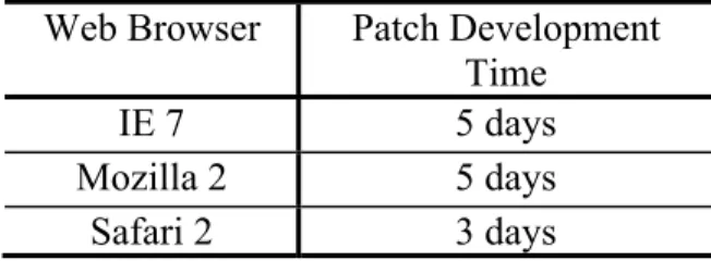
Patch development is another random process involved in patching and it refers to the process of making a fix for a known vulnerability by the vendor. Although speeding up, patch development is still a slow and time consuming process. Mean patch development time depends strongly on the vendor of the software. Symantec [12] reports mean patch development time for different web browsers. This time for Firefox and Internet Explorer is five days while for Safari it is three days.
We model vendor dependency and consider different mean patch development times.
D. Patch Testing and Deployment
Testing and deployment are the last phases of patching process. Pre-deployment testing is an important part of this process. Although it is recommended by previous studies, we discuss that it is a "double-edged sword". It can help correctly apply new patches and prevent introduction of new vulnerabilities. At the same time, it provides attackers a window of time to attack the system before testing is done. Deployment is usually fast compared to patch development and testing and it takes in the order of few minutes.
III. ANALYTICAL MODEL
In this section, we describe an analytical model to show the tradeoff between pre-deployment testing and the vulnerability of the system.
Although some studies describe vulnerability exploitation models (VEMs) [5], they are mostly limited to the specific software application under study and the specific attacker model. For instance, the exploitation model of a worm is different from that of a hacker targeting a specific organization. To keep the model general and
avoid such specificities, we do not use an exploitation model in this paper. We simply study vulnerabilities in a system and use the total number of open vulnerabilities at each time as a measure of the susceptibility of the system.
Assume that the number of new vulnerabilities found in a piece of software at time t is given by w(t). Note that w(t) is discrete in time; however, it can be approximated with little error with a continuous time function. Further assume that the cumulative number of vulnerabilities in a system is given by Ω(t). Ω(t) approaches a final value as times grows. This final value is the total number of vulnerabilities that will ever be discovered for that software. This function does not account for hidden vulnerabilities that are never discovered. Nonetheless if a vulnerability is forever undiscovered, it does not pose a threat and it is of little interest.
If we denote the patch develop time by TP and
pre-deployment testing time by TT, the total
number of open vulnerabilities at time t for a perfect patching system (in which patches introduce no new vulnerability) is given by:
(6) Equation (6) is obtained using the fact that every vulnerability discovered from time 0 to t-TP-TT is patched by time t. The only open
vulnerabilities are those for which no patch has developed yet or those under test.
We know that in reality patching is not perfect. In fact, each patch can introduce a new vulnerability to the system. Assume that on average, each untested patch introduces f new patches to the system. If f is greater than 1 (each patch introduces more than one new vulnerability on average), the system is unstable and the number of vulnerabilities grows indefinitely with time, so we study the system for 0≤f<1. If no testing is done, the number of new vulnerabilities by previous patches at time t is given by:
(7) Pre-deployment testing, however, can find some of these new vulnerabilities before applying the patch to the software. Unfortunately, to the best of
our knowledge, no real data is available for the number of new vulnerabilities discovered when testing a patch. However, these vulnerabilities are related to the same software version and the same vendor. As a result, we assume that they can be modeled using the vulnerability discovery trend for that software. Since the vulnerability discovery trend heavily depends on the software and its version, but it is accurate for a specific version of a software application, we believe that this assumption is valid.
Consequently, if each patch is tested for TT before
it is deployed, the number of new vulnerabilities introduced during testing is given by:
1 Ω Ω 0
1 Ω Ω 0
(8) Equation (8) is obtained from the fact that during testing Ω(TT) vulnerabilities are discovered in the
patch.
Some of the VDMs, have a small non-zero value at time 0 as an artifact. The term " Ω 0 " is added to the equation to compensate for that. If no such artifact exist, the multiplier can be simplified to
(1-Ω(TT)).
Note that equation (8) is correct for:
Ω(TT) - Ω(0) <1
This is because a patch on average has at most one new vulnerability.
The total number of open vulnerabilities at time t follows: 1 Ω Ω 0 Ω Ω , Ω Ω 0 (9)
In equation (9), for simplicity, the term
1 Ω Ω 0 is denoted by
The tradeoff can be observed from equation (9). By increasing the testing time (TT), the first term
grows because the window of exposure (integral limits) widens. On the other hand, the second term shrinks, because more testing results in more faults discovered.
The optimum pre-deployment testing at each time t, is the amount of TT that minimizes equation (9),
the total number open vulnerabilities at time t. If it is desired to have one optimum TT for all times and
remove the time dependency, the optimum TT is
given by:
| min
(10) In equation (10), L is the lifetime of the software. The optimum testing time minimizes the number of open vulnerabilities at all times. The upper bound of the integral in real-world applications is about two or three years. After this time, there are usually very few new vulnerabilities discovered for that software.
The analysis clearly shows that pre-deployment testing is not “always good.” There is a certain amount of testing which minimizes the number of vulnerabilities in the system. More testing increases the window of exposure for little gain and is detrimental to the security of the system.
IV. STOCHASTIC MODEL
This section describes the stochastic model of patch management. We simulate the stochastic model to find the optimal testing time using simulation as well.
The model includes vulnerability discovery as well as patch development, testing, and deployment processes.
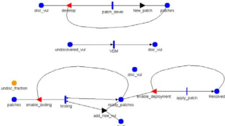
Patching is modeled in this paper using Stochastic Activity Networks (SANs) [11]. SANs are generalized form of stochastic Petri Nets (SPNs.) In addition to the components of SPNs, Stochastic Activity Networks (SANs) also include input gates (shown by triangles pointing left), output gates (shown by triangles pointing right), probabilistic cases (shown by small circles on activities), and instantaneous activities (shown by thin vertical
Fig. 1. The stochastic model of the patching system. lines). Input gates specify general enabling conditions, output gates define general completion functions, cases represent a probabilistic placement of tokens in the outputs with a specific probability for each case, and instantaneous activities denote activities that are completed in zero time. Mobius [6] is the tool used for simulation of the SAN model. All times in the model are expressed in months. Here, the details of the SAN model are explained and different choices of the parameters are discussed.
The model consists of three sub-models (Atomic models). They model vulnerability discovery, patch development, and patch testing/deployment processes.
The three sub-models are joined into a composed patch_system model using “Join” representation. This means that places with the same name in different sub-models refer to the same place in the composed model.
The first Atomic model, "vulnerability", expresses the vulnerability discovery model. In this model, two places contain undiscovered and discovered vulnerabilities and an activity (VDM) takes tokens from the former and put them in the later (figure 1). The initial marking of the undiscovered vulnerabilities is equal to the total number of vulnerabilities. We set the initial marking of the discovered vulnerabilities is one (and not zero) because making this marking zero also sets the discovery rate to zero and no vulnerability will ever be discovered.
For our simulation, we use the AML vulnerability discovery model; although, the stochastic model is general and any VDM can be used for it. The choice of AML model is because it fits the real vulnerability discovery data from the three web
Table 1: Patch development time for different browsers Web Browser Patch Development
Time
IE 7 5 days
Mozilla 2 5 days Safari 2 3 days browsers with small error.
To use the AML model, the rate of VDM activity is set to Ω Ω in which Ω is the marking of the discovered vulnerability and A and B are global variable. Note that VDM is a variable rate activity in which the rate is a function of the vulnerabilities discovered so far. In the stochastic model, we do not use the time domain solution for
Ω(t); rather, the underlying differential equation describing Ω (i.e. A Ω B Ω ) is used to model vulnerability discovery. This is one of the differences between the analytical model and stochastic model.
In our study, we assign real fitted values to A and B so that the model represents vulnerability discovery for Firefox, Internet Explorer, and Safari.
The second Atomic model describes patch development process (figure 1). Patch development time is software and vendor dependent. For the web browsers under study, the patch development times are set to those listed in Table 1. These times are reported for different browsers in the Symantec report [14].
Patch development continues until the total number of patches equals the number of discovered vulnerabilities. This is done using the input gate "develop".
The next element models the deployment phase of the patching process (see figure 1). If pre-deployment testing is being done on patches, a timed-activity moves new patches to tested patches ready for deployment. We change the testing time to find the optimal testing period. The distribution of testing activity is deterministic.
For a given testing period and faulty fraction (f), the fraction of patches that introduce a new vulnerability after testing is computed (
1 Ω Ω 0 ). This fraction is assigned to the second case of the “testing” activity which adds a new fault to the system. The first case of the activity is when the vulnerability is discovered and
it puts a new token to the “ready_patches” place (figure 1).
Applying a ready patch takes a small amount of time compared to development of the patch and pre-deployment testing, so it is modeled using an instantaneous activity named “apply_patch”.
V. SIMULATION RESULTS AND DISCUSSION This Section presents the results from the analytical model and different experiments on the stochastic model.
To study the effect of testing on the vulnerability of the system, we first need reliable data for the vulnerability discovery trend. For this, we use the National Vulnerability Database (NVD) and collect the vulnerabilities discovered in the three popular web browsers as well as the date of public disclosure.
For our study, we use Mozilla Firefox 2, Microsoft Internet Explorer 7, and Apple Safari 2 browsers. The reason for choosing these particular versions is that they are not old, at the same time, they are not the most recent versions (i.e. Firefox3 or Safari 3) for which very few vulnerabilities are discovered to this day. The vulnerabilities can be in the core of the browser or in any of its extensions or add-ons.
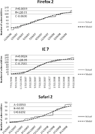
Then, we fit the AML model to these vulnerabilities by minimizing the mean-squared error. The cumulative number of vulnerabilities (Ω) for the three browsers from the real data as well as the fitted models and the parameter values are shown in figure 2.
We have simulated the stochastic model in Mobius [6] using the parameters from the three web browsers.
Figure 3 shows the cumulative number of vulnerabilities discovered obtained by simulating the stochastic model. The quantity plotted in this figure is the marking of (i.e. the number of tokens in) the place holding the discovered vulnerabilities (named “disc_vul” in the model).
The effects of different parameters such as faulty fraction (f), testing time (TT), and browser
dependency are studied in different experiments. In each experiment, the parameter under study is changed and other parameters are set to some fix value. This does not suggest that those fixed values are typical in any way. It is done to keep other
Fig. 2. Vulnerability discovery for different browsers. parameters invariant so that we can observe the effect of the parameter under study. Of course, in a real system, the behavior is a function of all these parameters.
To study the effect of faulty patches, the number of open vulnerabilities is plotted versus time for different f values in figure 4. The number of open vulnerabilities is the number of unpatched discovered vulnerabilities plus the number of faults introduced during previous patch deployments. For this experiment, no pre-deployment testing is done and the results are simulated for Firefox
2. Notice three facts from figure 4. First, the number of patches lags the number of discovered vulnerabilities. This is due to the time it takes for the vendor to develop new patches. Second, when there is no faulty patch (f=0), the number of open vulnerabilities goes to zero eventually. The non-zero value in the middle is the difference between the number of vulnerabilities and patches. Third, for faulty patches, there are always residual faults that remain in the system.
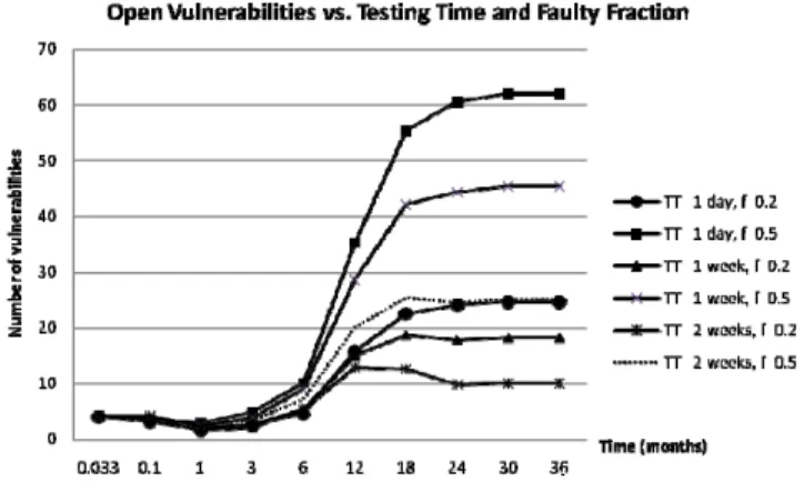
The next experiment, studies the effect of testing
Fig. 3. Vulnerability discovery from the stochastic model. on the number of open vulnerabilities. This experiment is done for two f values (0.2 and 0.5) and three testing periods (two weeks, one week, and one day). Internet Explorer 7 is used as the model. The results are shown in figure 5. Observe that for a given time, a specific testing period minimizes the area under the curve from zero to that time which is the total number of open vulnerabilities over that time. This amount of pre-deployment testing is the optimal testing.
The parameters used in the experiment are arbitrary values chosen for demonstration of the effects only. The exact optimal testing period for a given faulty fraction can be obtained from equation (10). In the next section we show that the results from the analytical model matches those obtained here from simulation.
Intuitively, more testing or smaller faulty fraction results in the smaller number of residual vulnerabilities in the system. Interestingly, two weeks of testing with 50% fault result in the same residual vulnerability as one day of testing with 20% fault. This means that in order to compensate for faultier patches, a lot more testing has to be done. We verify this result in the next section.
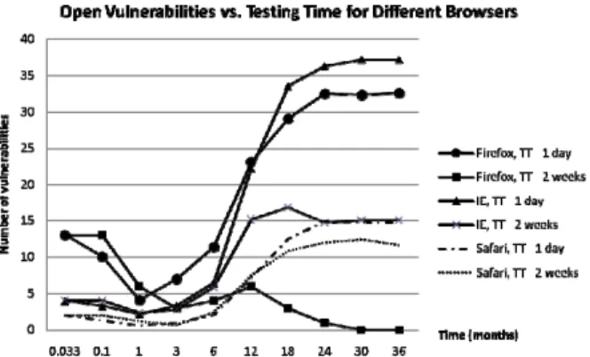
Finally, the last experiment studies the software dependency of pre-deployment testing. For this experiment, we plot the number of open vulnerabilities at each time for the three web browsers given a faulty fraction of 0.3 and testing periods of two weeks and one day. The results are shown in figure 6. The patch development times for this experiment are five days for Firefox and IE and three days for Safari. These times are taken from the Symantec report [14].
Fig. 4. The number of open vulnerabilities for various faulty fractions.
There are two observations to be made for this experiment. First, the evolution of open vulnerabilities over time is highly dependent on the software (in this case the web browser.) Second, there is a common trend between different web browsers and testing times. The number of open vulnerabilities is high at the beginning before the vendor gets a chance to develop patches for the initial problems. It shrinks to a minimum between one to six months after the initial phase is passed. It then grows rapidly or peaks at around one year into the process. This sharp growth is because users become more familiar with the software at the rate of vulnerability discovery is very high at this point. Finally, it approaches the terminal after about three years.
VI. VERIFICATION AND VALIDATION
In this section, we validate the sub-models used in the analytical and stochastic models in this paper. Furthermore, we verify the results obtained by simulating the stochastic model using the analytical model.
First, to validate the vulnerability discovery model, we calculate the mean squared error (MSE) of the fitted AML model compared to the actual data from the vulnerability database (figure 2.) The MSE for Firefox, IE, and Mozilla are 27.5, 22.7, and 11.7 respectively. Also the percentages of error for these browsers are 6.94%, 5.50%, and 11.74% respectively. The errors for IE and Firefox show that the model is a good fit for the actual data. For Safari, the error is little larger because of smaller number of samples and cumulative public
Fig. 5. The number of open vulnerabilities for various testing times.
disclosure of vulnerabilities which results in a staircase-like trend.
Next, we validate the stochastic vulnerability discovery model (figure 3) by calculating its error from the actual data. The percentages of error for stochastic models of Firefox, IE, and Safari are 12.0%, 12.8%, and 12.5%. Most of the error is because of the initial error in the model for the first two samples (i.e. one day and three days.)
To verify the simulation results, we compare them to those obtained from the analytical model. Equation (10) gives the optimal pre-deployment testing time for any period of lifetime. It is important to notice that the optimal time depends on the goal one wants to achieve. For instance, the goal of minimizing the number of open vulnerabilities over the two year lifetime of the software results in a different optimal time than that of minimizing the number of open vulnerabilities at a specific time. In the analysis provided here, without loss of generality, assume that the goal is to minimize the number of open vulnerabilities over the two year lifetime of the software. Since a new version of the browser is introduced after two years, this can be a meaningful goal.
First, we solve the analytical model for the second simulation experiment. The model is solved for f=0.2 and the three testing times (one day, one week, and two weeks.) By solving equation (9), the total numbers of open vulnerabilities over two years for the three experiments are 317.3, 262.2, and 195.9 respectively. These values do not refer to real vulnerabilities; rather, they are the summation of all possible windows of exposure. The values from the analytical model and the stochastic model agree in
Fig. 6. The number of open vulnerabilities for the different browsers.
what they suggest. That is, two weeks of testing is better than one week or one day. The reason becomes apparent when we explicitly solve the analytical model for IE 7 to find the optimum testing time. By solving equation (10), the optimum testing time is 0.7845 months or about 23 days (total open vulnerabilities over two years=116.8). That is why two weeks of testing achieves better results than one week or one day in the simulation. In fact, analytical model give insight to the results obtained in the simulation section.
In addition, we verify the result found in the second experiment that 20% fault with one day of testing has the same number of residual vulnerabilities as 50% fault with two weeks of testing. From the analytical model, and by substituting the actual values for IE 7, the value of
1 Ω Ω 0 is the same for f=0.2 and TT=0.033(months) as f=0.5 and TT=0.5
(months). This quantity is what we called α and shows the residual vulnerability. The analytical value obtained for α in both cases is 24.2 which again is the same value from the simulation in figure 5.
Finally, we obtain the optimum testing time for all of the web browsers for the last simulation experiment. The optimum TT for IE, Firefox, and
Safari (f=0.3) are 0.784 month (=23 days), 0.353 month (=10 days), and 1.928 month (=57 days) respectively. This verifies why the residual vulnerability after two weeks of testing for Firefox is zero, but for IE and Safari it is not (figure 6.) Two weeks of testing is greater than the optimal testing time of Firefox, but smaller than those of IE or Safari. Hence, α is zero for Firefox while it is non-zero for IE and Safari.
It is important to realize what the verifications in this section suggest. They do not prove that the analytical model and the models used in the simulation are correct. On the other hand, they show that these models, capturing medium-level details of the system, indicate the same tradeoff and they match in what they suggest. It is possible to come up with more sophisticated models to capture low level details of a patching system. However, the fundamental tradeoff always exists in the system: pre-deployment testing results in more exposure and smaller new vulnerabilities.
By comparing the results with the actual real-world vulnerability data for different browsers, we have shown that these medium level models can capture the reality with a margin of about 12% error.
VII. RELATED WORK
Patch management and vulnerability trend analysis has recently attracted attentions in IT environments. Symantec report various vulnerability trends as well as vendor patch development times along with much more information in its annual report [14]. Rescorla [10] describes the life cycle of a vulnerability and its different phases. Gerace and Cavusoglu identify seven different elements necessary for a successful patch management process: senior executive support, dedicated resources and clearly defined responsibilities, creating and maintaining a current technology, identification of vulnerabilities and patches, scanning and monitoring the network, pre-deployment testing of patches, post-pre-deployment scanning and monitoring.
There have been several works on modeling patching related processes. They describe different probabilistic vulnerability discovery models (VDM) [1] [2] [3] [4] [9]. These works try to describe the process of vulnerability discovery using simple probabilistic models.
Another set of work focuses on vulnerability exploitation models (VEM). They describe exploitation of known vulnerabilities again using probabilistic models. [5]Browne [5] investigates exploitation of some specific vulnerabilities and builds a modeling scheme based on such data.
VIII. CONCLUSIONS AND FUTURE WORK Patch management has become one of important security issues in IT departments. New vulnerabilities introduced to systems during a faulty patching process add to the complexity of successful patch management.
This work investigated the effect of pre-deployment testing on the overall security of the system under different operational circumstances. We have developed an analytical model as well as a stochastic model which we solve using simulation. Results suggest that there is an optimal pre-deployment testing that results in minimum number of open vulnerabilities.
We plan to use more detailed models and empirical distributions to describe vulnerability discovery process.
In addition, more sophisticated model for patch development time can result in error reduction. Empirical data can be used to express the probability distribution of this delay.
Finally, real experiments on testing patches can result in more accurate models for the number of fault discovered during testing.
REFERENCES
[1] O. H. Alhazmi, Y.K. Malaiya, "Modeling the vulnerability discovery process" , 16th IEEE International Symposium on Software Reliability Engineering, 2005, page(s): 10 pp, 8-11 Nov. 2005
[2] O. H. Alhazmi, Y. K. Malaiya, “Prediction Capability of Vulnerability Discovery Models”, In Proc. Reliability and Maintainability Symposium, January 2006.
[3] O. H. Alhazmi and Y.K. Malaiya, “Quantitative Vulnerability Assessment of Systems Software,” In Proc. Annual Reliability and Maintainability Symposium, 2005. pp. 615 –620.
[4] R. J. Anderson, “Security in Opens versus Closed Systems—The Dance of Boltzmann, Coase and Moore,” Open Source Software: Economics, Law and Policy, Toulouse, France, June 20-21, 2002.
[5] H.K. Browne, W. A. Arbaugh, J. McHugh, W.L. Fithen, "A trend analysis of exploitations", In Proceedings of 2001 IEEE Symposium on Security and Privacy, page(s): 214-229, 2001
[6] D. D. Deavours, G. Clark, T. Courtney, D. Daly, S. Derisavi, J. M. Doyle, W. H. Sanders, and P. G. Webster, "The M¨obius Framework and Its Implementation", IEEE Trans. on Software Engineering, 28(10):956–969, Oct. 2002.
[7] T. Gerace, H. Cavusoglu, "The critical elements of patch management". In Proceedings of the 33rd Annual ACM SIGUCCS Conference on User Services, SIGUCCS '05.
ACM Press, New York, NY, 98-101, November 06 - 09, 2005
[8] N. Loriant, M. Segura-Devillechaise, J.-M. Menaud, "Server protection through dynamic patching", In Proceedings of The 11th Pacific Rim International Symposium on Dependable Computing, page(s): 7 pp., 12-14 Dec. 2005
[9] J.D. Musa and K. Okumoto, “A logarithmic Poisson execution time model for software reliability measurement,” In Proc. 7th International Conference on Software Engineering, Orlando, FL, 1984, pp. 230-238. [10] E. Rescorla, "Is finding security holes a good idea?",
Security & Privacy Magazine, IEEE, Vol 3, Issue: 1, page(s): 14- 19, Jan.-Feb. 2005
[11] W. H. Sanders, J. F. Meyer, "Stochastic Activity Networks: Formal Definitions and Concepts", In E. Briksma, H. Hermanns, and J. P. Katoen, editors, Lectures on Formal Methods and Performance Analysis, pages 315–343. Springer-Verlag, Berlin, 2001.
[12] "Symantec Internet Security Threat Report", Trends for January 06–June 06, Volume X, Published September 2006
[13] E. Byres, D. Leversage, and N. Kube, “Security incident and trends in SCADA and process industries:A statistical review of the Industrial Security Incident Database (ISID),” White Paper, Symantec Corporation, 2007
[14] D. Turner, S. Entwisle, E. Johnson, M. Fossi, J. Blackbird, D. McKinney, R. Bowes, N. Sullivan, C. Wueest, O. Whitehouse, Z. Ramazan, J. Hoagland, and C. Wee, “Trends for January–June 07,” Symantec Internet Security Threat Report, Volume XII, 2007