How to Understand High Food Prices

DIPARTIMENTO DI ECONOMIA

_____________________________________________________________________________

How to Understand High Food Prices

Christopher L. Gilbert

_________________________________________________________ Discussion Paper No. 23, 2008

The Discussion Paper series provides a means for circulating preliminary research results by staff of or visitors to the Department. Its purpose is to stimulate discussion prior to the publication of papers.

Requests for copies of Discussion Papers and address changes should be sent to:

Dott. Luciano Andreozzi

E.mail luciano.andreozzi@economia.unitn.it Dipartimento di Economia

Università degli Studi di Trento Via Inama 5

How to Understand High Food Prices

Christopher L. Gilbert

CIFREM and Department of Economics, University of Trento, Italy and Department of Economics, Birkbeck College, University of London, England.

Initial draft: 9 July 2008 This revision: 17 November 2008

JEL subject code: Q11

Keywords: Food prices, commodity prices, money, futures markets

Abstract

Commodity price booms are best explained by macroeconomic rather than market-specific factors. I argue that the rise in food prices over 2007 and the first half of 2008 should be seen as part of the wider commodity boom which is largely the result of rapid economic growth in China and throughout Asia in a context of loose money and in which, because of previous low investment, supply was inelastic. The demand for grains and oilseeds as biofuel feedstocks was the main cause of the price rise but macroeconomic and financial factors explain its extent. The futures market may be an important monetary transmission mechanism, but it is commodity investors, not speculators, who, by investing in commodities as an asset class, may have generalized prices rises across markets.

This paper was prepared for the conference “The Food Crisis of 2008: Lessons for the Future”, Wye College, 28 October 2008. The initial version of this paper was given at an FAO Group of Exports meeting on High Food Prices, Rome, 9-10 July 2008. That meeting marked the peak of the food price cycle. A subsequent version of the paper was given at the Dipartimento di Economia Politica, Università degli Studi di Milano, Bicocca, 1 October 2008. I am grateful to Don Mitchell, Colin Thirtle, members of the FAO Group of Experts and participants at the Bicocca and Wye meetings.

Address for correspondence: Dipartimento di Economia, Università degli Studi di Trento, Via Inama 5, 38100 Trento, Italy; cgilbert@economia.unitn.it and c.gilbert@bbk.ac.uk

1. Introduction

The prices of food commodities doubled in real terms from 2005 to mid 2008.1 Taking figures up to the July 2008 peak, the major increases were palm oil (140%), rice (110%), maize (102%), wheat (101%) and soybeans (86%). These price rises were general across the range of agricultural products with only a small number of exceptions – sugar prices rose by only 1%. Figure 1 illustrates. 0 50 100 150 200 250 300 2000 2001 2002 2003 2004 2005 2006 2007 2008 (d e fl a te d , 2 0 0 0 = 1 0 0 )

Maize Palm Oil

Rice Soybeans

Sugar Wheat

Jan-July

Figure 1: Major agricultural prices, 2000-082

The rises in food prices took place in the context of a general rise in commodity prices led by energy and metals. This is evident from the IMF indices plotted in Figure 2. The figure shows the 19% rise in real food prices and the 25% rise in beverage prices to have been modest in relation to the much higher rises in energy and metals prices (89% and 125% respectively).

1

I confine myself in this account to discussion of food commodities and do not consider the transmission of changes in these prices into retail food prices.

2

The prices of agricultural raw material prices, which cover natural fibres and natural rubber, fell in real terms over the same period.

Figure 2: IMF Commodity price indices, 2000-083

The entire range of commodity prices saw sharp falls over the second half of 2008, and in particular from September in the “post-Lehman” months. Most notably, the price of crude oil has halved from over $140/bl to under $60/bl. Food prices have not been immune to these developments. Chicago corn (maize) prices, for example, fell from a June 2008 peak of 700c/bu ($226/ton at 2006 values) to 400c/bu ($130/ton at 2006 values).

The paper is structured as follows. In Section 2, I discuss why prices may be more responsive to shocks in boom situations than would be the case in normal times. I compare the recent (2005-08) boom in agricultural commodity prices with the 1972-74 boom. I suggest that, if we are to understand commodity price booms, we need to move beyond market-specific factors and consider macroeconomic and financial factors which operate across large numbers of markets. In section 3, I use simple econometric methods to attempt to isolate the main causal

3

Source: as Figure 1. The 2008 figure is the average for the seven months January-July.

75 100 125 150 175 200 225 250 275 2000 2001 2002 2003 2004 2005 2006 2007 2008 Foods Beverages

Agricultural raw materials Metals

factors at work. I show that economic growth and changes in the world money supply have played an important role in moving agricultural prices. These have been under-played in most recent discussions of agricultural prices. There is weaker evidence that the oil price and the level of futures market activity have also been important over the more recent period. Exchange rate changes have not been important.

Sections 4 to 7 amplify these arguments. Section 4 looks at biofuel demand. This has had a direct impact on maize and oilseed prices. Through incentivizing change is land use, it has had indirect effects on wheat and soybean prices, and on meats through use of maize as animal feed. Because biofuels still only account for a small proportion of total energy consumption, the long run demand for grains and oilseeds for energy purposes becomes infinitely elastic at a price dependent on the oil and fertilizer prices. This generates a much closer link between oil prices and the prices of agricultural food commodities now than was the case in the past.

In Section 5, I look at the impact of rapid growth in China and other parts of Asia on agricultural prices. Although the direct impact of Chinese growth on food prices is small, I argue that the indirect impact is likely to have been large. This indirect impact comes largely through increasing the sensitivity of agricultural prices to demand shocks by decreasing supply responsiveness. Production costs (transport costs and fertilizer prices), the effects of higher energy prices in stimulating production of biofuels and the effects of higher energy and metals prices in stimulating interest in commodity investment are instrumental in this process.

In section 6, I turn to monetary growth, a factor which has received relatively little attention in the current discussion. The channels through which monetary growth is transmitted into agricultural prices are diverse and also variable over time. Further, it is important to distinguish between unilateral monetary expansion in a particular economy, which will primarily affect agricultural prices through exchange rate depreciation, and expansion at the global level, which may leave exchange rates unaffected. Interest rate effects on agricultural prices may be more pronounced in periods of excess supply rather than in booms. The main effects of monetary expansion in the 2006-08 boom may have come through the generalized effects of monetary growth on asset prices.

Agricultural futures markets are one channel through which monetary growth may have impacted food commodity prices. I discuss this possibility in Section 7. Contrary to the efficient markets view, futures markets can distort prices. Speculation can lead to self-fulfilling

bubble-type phenomena, although the evidence is that such events tend to be short-lived in the commodity context. Nevertheless, I do find some evidence of likely bubble behaviour in recent agricultural price movements. Index-based commodity investments are more problematic. These can be large relative to the size of agricultural futures markets which, in any case, are not always highly liquid. Although less evidence is available, it does appear that this activity can put upward pressure on prices and may transmit price movements from one market to another, both within the agricultural sector, and also from energy and metals markets to food commodities. Section 8 concludes.

2. Commodity price booms

The commonality of price rises in energy, metals and foods documented in the introduction, and the commonality of their subsequent falls, is unlikely to have been coincidental. It may have arisen in either or both of two ways. The first is through common causation – a common set of driving factors (dollar depreciation, Asian demand growth etc.) may underlie price rises across a range of commodities, foods included. The second mechanism is links across markets – high energy prices may raise costs throughout the commodity producing industries, or the belief that commodities may be good investments in a stagflationary environment may lead investors to take positions across the entire range of commodity markets, again including food commodities.

Most explanations of recent commodity price movements focus on shifts in the demand curve – increased demand for energy and metals in the rapidly growing Asian economies and increased biofuels demand for grains and oilseeds. Elementary economic theory tells us that rightward shift a demand curve will, in almost all circumstances, lead to a price rise. However, the extent of the rise depends on the slope of the supply curve. If supply is very elastic, the price rise is modest. If supply is less responsive, the price rise is more substantial. If supply is very inelastic, even a small shift in demand can have a large price impact.

There are two reasons why supply curves may be inelastic in priced booms. First, booms tend to come after periods of low investment. Prior to 2005, commodity prices, and agricultural commodity prices in particular, had been low for two decades. In energy and metals, the effects were seen in low levels of profitability and low share prices, both of which limited the ability of firms to raise funds for investment. In agriculture, low levels of investment appear to have resulted in a slowdown of productivity growth and reduced the capacity of world agriculture to

respond to current shocks. The World Bank’s 2008 World Development Report called for a reprioritization of agriculture in developing countries development strategies (World Bank, 2008a).

The second factor limiting supply responsiveness is the fact that markets are linked. I illustrate this in Figure 3. Consider a demand shock D→D’ which is specific to an individual

agricultural market. The appropriate supply curve in that market is S. Factors are drawn in from other markets and supply is elastic, with the result that the demand shock leads to the small price rise p1- p0. If, instead, the demand shock is common across a range of agricultural markets, the

position becomes more complicated. First, there may be cost increases as outputs from one sector are used in others, e.g. energy inputs into agricultural production. This is reflected in the upward shift of the supply curve to S’. Second, because the possibilities for reallocation of land and other inputs across crops are limited in the context of a common demand shock, additional factors are only available at considerable extra cost making supply inelastic. The supply curve becomes less elastic, rotating to S”. The result is that the same demand shock in terms of the market in question will lead to the much larger price rise p2 - p0.

Figure 3: Price responses to idiosyncratic and common demand shocks

This inter-relationship across markets was most evident in metals and energy where delivery times on essential items of equipment escalated from a typical six months to three years

p0 p1 p₂ S S” D D’ S’

or longer. Partly as a result, production costs for new developments increased in line with prices. In the remainder of this paper, I will argue that it has also been a feature of agricultural markets.

Standard “additive” explanations of commodity price movements run in terms of price responses to a set of supply and demand shocks. If response coefficients are constant across the sample, price responses in the boom to may appear disproportionately large relative to normal times. This will tend to strain standard explanations of price changes in terms of market-specific factors. Second, and by implication, changes in commodity prices may be better explained by aggregative or macroeconomic factors which affect the entire range of commodity markets.

Many commentators have noted the parallels with between the 1973-74 and 2005-08 commodity price booms – see, for example, Radetzki (2006). History should not be expected to repeat itself precisely but the important lesson is that, as in 2006-08, the 1973-74 boom in agricultural prices in 1973-74 occurred against the backdrop of a general rise in commodity prices. The causes of the 1973-74 boom were authoritatively discussed by Cooper and Lawrence (1975). Then, as more recently, the markets were inter-related.

Figure 4: Commodity Prices 1970-76 (left, grains; right, coffee and sugar)4

Figure 4 charts (left panel) monthly real prices for grains over the seven year period 1970-76, and also (right panel) does the same for coffee and sugar. In both cases, the real petroleum (WTI) price is included, as a broken line, for comparison.

• Both took place in the context of enormous world liquidity resulting in part from large U.S. trade deficits and loose monetary policies.

4

Source: International Monetary Fund: International Financial Statistics. Petroleum –WTI; grains – US; coffee – other milds (New York), sugar – free market.

0 100 200 300 400 500 Ja n-70 Jul-7 0 Ja n-71 Jul-7 1 Ja n-72 Jul-7 2 Ja n-73 Jul-7 3 Ja n-74 Jul-7 4 Ja n-75 Jul-7 5 Ja n-76 Jul-7 6 (1 9 7 0 = 1 0 0 ) Petroleum Wheat Maize Soybeans 0 100 200 300 400 500 Ja n-70 Jul-7 0 Ja n-71 Jul-7 1 Ja n-72 Jul-7 2 Ja n-73 Jul-7 3 Ja n-74 Jul-7 4 Ja n-75 Jul-7 5 Ja n-76 Jul-7 6 (1 9 7 0 = 1 0 0 , c o ff e e , p e tr o le u m ) 0 300 600 900 1200 1500 (1 9 7 0 = 1 0 0 , s u g a r) Petroleum Coffee Sugar

• In both cases, oil prices jumped sharply upwards.

• Both booms ended sharply with the onset of recession, in the second quarter of 1974 and third quarter of 2008 respectively.

• Metals prices rose strongly in both booms. Coffee and cocoa were sidelined in both cases.

• The sugar price, which jumped very sharply in 1973, played an analogous role in 1973-74 to that of the rice price in 2007-08.5

• Rapid growth in the Japanese economy was a major driving force in the 1973-74 boom,

as was rapid growth in the Chinese economy in the more recent period. However, Japan was probably not as important in the 1970s as China has been in the current decade. There were also important differences. Firstly, the 1973-74 boom was shorter than the 2003-08 commodity price boom. Secondly, although grains participated in the booms, they led in 1973-74, ahead of the rise in oil prices (see Figure 4), but lagged in 2003-08 where the rise came only at the end of the boom.

There is a tension evident in analysis of both the 1973-74 boom and the 2003-08 boom between focus on market-specific factors (poor harvests, biofuels, export restrictions etc.) and discussion of global factors (China, world monetary conditions, etc.). Market-specific factors can explain why the prices of some products rose and others did not, but macroeconomic factors explain the extent of the price rises. When we aggregate across the entire group of agricultural food commodities, we will find that it is the macroeconomic and financial factors that account for the price booms such as those of 1972-72 and 2005-08.

5

It is a feature of both the rice and sugar markets that the bulk of transactions are at contracted or subsidized prices and that only a small proportion of commerce takes place at free market prices which therefore tend to be highly volatile. There was no significant shortage of rice in aggregate in 2007-08. The jump in rice prices in 2007 resulted from the decision by the Government of India to ban rice exports, possibly to hold down domestic food costs in the context of rising wheat prices. The Indian ban limited supply to the residual free market and, as prices rose, other exporters followed the Indian example. Rice-importing countries, most notably the Philippines and Haiti, were forced to pay disproportionately high prices. The situation was eventually saved when the Japanese government announced that it would release part of its rice food security stockpile onto the world market. I do not pursue this incident or its implications further in this paper. For discussion see World Bank (2008b).

3. Econometric analysis

In this section, I use simple econometric methods to investigate the possible importance of a number of macroeconomic and financial factors which have been held to influence agricultural prices.

• There is general agreement that changes in the oil price O are likely to feed through into other commodity prices. I examine this at greater length in Section 4.

• Shocks to aggregate demand feed directly into food commodity prices. Unlike supply shocks, these tend to be common across the broad range of commodities. I discuss demand shocks at greater length in section 5. In what follows, I measure aggregate demand Y by an estimate of the level of world GDP. Importantly, this measure includes GDP for China, India and Russia as well as for the advanced economies. National currencies are converted into U.S. dollars using PPP exchange rates taken from Ahmad (2003).

• The 1973-74 boom occurred shortly after the 1972 break-down of the Bretton Woods fixed exchange rate system. Subsequently, there was a substantial increase in international liquidity which, in the absence of clear nominal anchors, resulted in rapid inflation. Commodities were seen as a safe real asset in a period of unreliable monetary values (Cooper and Lawrence, 1975). This suggests examination of the impact of changes in world money supply M.

• Agricultural commodity prices are denominated in terms of the U.S. dollar. Changes in the value of the dollar should therefore change dollar prices as documented in Ridler and Yandle (1972) and Gilbert (1989). Abbott et al. (2008) emphasize the importance of this factor. I construct a measure X of the value of the U.S. dollar against a basket of currencies.

• It is possible that activity on agricultural futures markets affect agricultural commodity prices. IFPRI (2008) has suggested that commodity speculation may be a contributory factor in recent agricultural price rises and has suggested market-calming regulations. We explore this hypothesis in Section 7. Here I proxy futures market activity by trading volume V on the three Chicago grains futures markets.

All monetary variables are deflated by the U.S. GDP deflator. Variable definitions are given in an appendix. 6

I use Granger non-causality tests to isolate the principal causal factors at work in the two booms. The tests use the five ADL (Autoregressive Distributed Lag) equations

(

)

∑

∑

These choice of lag length reflects prior tests from a more general specification with a uniform specification of 9 lags. In each case, the null hypothesis of Granger non-causation is

0 : 1 5 0

J J J

H β = = β =… (2)

and the alternative is its negation. The null and alternative hypotheses are unchanged. Tests are reported for the entire sample 1971q3 – 2008q2 and also for the first and second halves of the sample separately. Results are reported in Table 1.

Table 1

Granger Non-Causality Tests 1971q1-1989q4 F(5,65) 1990q1-2008q2 F(5,63) 1971q1-2008q2 F(5,139) Money supply M 3.57 [0.7%] 0.95 [45.5%] 4.20 [0.1%] Oil price O 2.92 [1.9%] 1.31 [27.1%] 0.86 [51.1%] Futures volume V 1.13 (35.6%) 1.45 [22.0%] 2.13 (6.6%)

Dollar exchange rate X 0.93

[47.0%] 0.13 [98.7%] 1.05 [39.0%] GDP Y 1.55 [18.6%] 2.73 [2.7%] 3.31 [0.8%] Dependent variable: Change in deflated agricultural foods price index ∆lnP

All variables enter are log differences.

Tail probabilities are given in "[.]" parentheses.

First consider the tests over the entire sample. The tests reject Granger non-causality for changes in the world money supply and for changes in world GDP, but fail to reject for the oil

6

ADF tests (not reported) confirm that all variables are I(1). I also considered world foreign exchange reserves (source: IMF, International Financial Statistics). This gave similar but less powerful results as the world money supply variable. In relation to futures activity, I also considered open interest on the three grains markets. Results are similar to those reported for futures volume.

price, dollar exchange rate and futures volume (the final result being marginal). The tests for the two sub-samples have less power. Looking at the first half of the sample, which goes to the end of 1989, the tests confirm the role of the money supply but also reject non-causality for changes in the oil price. By contrast, in the second half of the sample, there single rejection of non-causality at the 95% level is for GDP growth. Exchange rate changes are not seen as important in either sub-sample or in the entire sample.

Granger non-causality test rejections are vulnerable to the criticism that the causal link may be indirect. Failures to reject are vulnerable to the criticism that some causal links may only be apparent if other causal variables are included in the tests equation. These considerations motivate corroboration of Granger non-causality test results using Vector AutorRegression (VAR) block exogeneity tests, which are the multivariate analogues of bivariate Granger non-causality tests. We use a VAR(3) specified as7

3 3 3 0 1 1 1 3 3 3 1 1 1 ln ln ln ln ln ln ln M O t i t i i t i i t i i i i V X Y i t i i t i i t i t i i i P P M O V X Y v − − − = = = − − − = = = ∆ = α + α ∆ + β ∆ + β ∆ + β ∆ + β ∆ + β ∆ +

∑

∑

∑

∑

∑

∑

VAR(3) Block Exogeneity Tests

1971q1-1989q4 F(3,57) 1990q1-2008q2 F(3,55) 1971q1-2008q2 F(3,131) Money supply M 2.23 [9.4%] 0.79 [15.5%] 5.83 [0.1%] Oil price O 1.90 [14.0%] 1.81 [15.7%] 0.18 [90.8%] Futures volume V 0.24 (87.0%) 1.80 [15.8%] 0.24 (87.0%)

Dollar exchange rate X 0.88

[45.5%] 0.73 [54.0%] 1.86 [13.9%] GDP Y 0.60 [62.1%] 2.02 [12.2%] 2.96 [3.5%] Dependent variable: Change in deflated agricultural foods price index ∆lnP

All variables enter are log differences.

Tail probabilities are given in "[.]" parentheses.

7

The choice of a VAR(3) was made after testing down from a VAR(5). A shorter lag length increases power.

The tests for the entire sample confirm the importance of money and GDP growth, as anticipated in the Granger non-causality tests in Table 1. No role is seen for other factors. The results from the two sub-samples suffer from lack of power and do not support any firm conclusions. Overall, these results support the role of world monetary and liquidity factors as a driver of agricultural food commodity prices. They do not assign any major role to exchange rate changes. The oil price and GDP growth are seen as having a positive impact on agricultural prices in the more recent period but not in the nineteen seventies. Futures market activity is not seen as having a major impact on prices in either period.

These results should be interpreted with caution. Failure to establish a causal relationship cannot be taken as implying that the variable in question did not influence prices, but rather that, if there was such a relationship it was either not consistent over time or that it was insufficiently large to be adequately distinguished from the other factors, including random factors, which affect these prices. It is clear, for example, from casual observation that exchange rate changes do affect agricultural commodity prices. However, exchange rates may not have moved sufficiently to have been an important determinant of major changes in agricultural prices. In section 7 I document evidence of effects of futures market activity on agricultural prices but these appear episodic and activity may not be well-captured by trading volume reflects seller-initiated as well as buyer-seller-initiated trades. However, where clear causal relationships are encountered, as in the case of monetary and GDP growth, we should take these as evidence that these factors have been responsible for a significant part of aggregate agricultural price movements over the period in question.

4. The oil price and biofuels

Increases in oil prices will result in higher food production costs. One link is through nitrogen-based fertilizers. A second is through transport costs. However, agriculture is not highly energy-intensive and although there is a small positive correlation between the levels of real oil prices and real food prices, price changes are poorly correlated. Baffes (2007) estimates the pass-through of oil prices into agricultural commodity prices as 0.17. Mitchell (2008) estimates that the combined effects of higher energy and transport costs have been to raise production costs in U.S. agriculture by 15%-20%. Overall, therefore, we may see the agricultural supply curve as having only shifted upwards to a small extent as the result of higher oil prices.

More important is that diversion of food crops for biofuels production has raised potential demand for food commodities. Mitchell (2008) suggests that biofuels demand is responsible for the largest part of the rise in food prices but resists the temptation to quantify this share. Abbot et

al (2008) concur with this view.

Production conditions differ from one country to another and so, unsurprisingly, different countries have chosen to use different crops as biofuel feedstocks. Maize is the main feedstock crop in the U.S., oilseeds hold that position in Europe, Brazil uses sugar cane, Thailand uses cassava while palm oil has been most important in the remainder of south Asia. These feedstocks also benefit from both mandates and subsidies in the U.S. and E.U.

Maize is principally used in the developed world as an animal feed. The figures in Mitchell (2008) show that the global use of maize for feed has risen by 1.5% over the four years 2004-07 while its use as a biofuel feedstock has gown by 65% over the same period. 70% of the increase in maize production over this period has gone into biofuels. This is a substantial increase in demand and will have had a direct impact on maize prices. Farmers respond to changes in the relative prices of different grains by changes in land use. The major expansion in maize production has been largely at the expense of soybeans – see Mitchell (2008) who documents a 23% increase in the area devoted to maize in the United States in 2007 simultaneously with a 16% decline in soybean area. Although soybeans are not directly used as a biofuel feedstock, this shift in land use suggests that biofuel demand for maize was a major contributory factor to the rise in soybean prices.

Price rises for oilseeds, the main European and Asian biofuel feedstock, have been substantial. Vegetable oils are widely used for cooking throughout the developing world. As with maize, the major impact of biofuel demand for oilseeds has probably been through its effects on land use. Mitchell (2008) documents that the eight largest wheat exporting countries expanded the area devoted to rapeseed and sunflower by 36% over the period 2001-07 while wheat area in the same countries fell by 1%. As with soybeans, it is not economic to use wheat as a biofuel feedstock. However, biofuels demand for oilseeds and maize has pre-empted the possibility of production increases to meet rising demand. It therefore seems likely that biofuels demand is a major contributory factor to the rise in wheat prices. Consistently with this view, the rise in palm oil and maize prices, where there has been a direct effect from biofuels demand, has exceeded that of soybeans and wheat where the effect is indirect.

Schmidhuber (2006) provides a framework in which we can look at biofuels as a transmission effect from oil the oil market to agricultural food markets. He argues that the prices of crude oil and fertilizers define a break-even price for each of sugar cane, maize and palm oil at which production of ethanol or biodiesel yields zero profit. At lower prices, it will pay to divert production away from food and towards energetic uses. In the long run, demand for these commodities in a free trade world effectively becomes infinitely elastic at these break-even prices. (The infinite elasticity assumption follows from the small likely share of biofuels in total energy supplies). Subsidies and tariffs, such as the U.S. tariff on imported ethanol, complicate these relationships but the principles remain clear. The consequence is that the grains and oilseed markets become integrated into the energy market and shocks to energy prices are transmitted to food commodities. This is what we have seen in 2006-08. Furthermore, since refining biofuel capacity is relatively inexpensive, price transmission from the oil market to food markets can be rapid.

Figure 5: Biofuels demand and grains prices

None of this implies that use of food commodities for biofuels inevitability implies food commodity prices as high as those seen over the 2006-08 boom. On the other hand, it is also true that prices are likely to remain higher than those seen prior to 2006. In Figure 5, the demand for grains for food uses is D and the supply curve is S. In the absence of biofuels demand, the grains price is p0. Demand for grains as a biofuel feedstock is infinitely elastic at price p1 which

depends on the oil and fertilizer prices. If this price is less than p0, the potential biofuels demand D S p0 p1 Q S’

fails to materialize and there is no price impact. If the price of oil is higher, of fertilizer prices are lower, such thatp1 >p0, the grains price rises and biofuels demand squeezes out some food demand. It follows that biofuels demand can raise but cannot reduce food commodity prices. As oil and fertilizer prices vary, on average the effect will be positive. Under the infinite demand elasticity assumption, increased grains supply (the shift from S to S’ in Figure 5) will not change this situation but will lead to increased consumption of grains as biofuels without further reduction in grains consumption in foods. This appears to be what has happened in Brazil where increases in sugar cane production have permitted increases in the production of both refined sugar and ethanol.

This discussion suggests that, although the direct impact of a rise in the oil price on agricultural prices will likely exceed the direct pass-through into production costs. Because the rise in costs is common across all agricultural commodities, there is little scope for reallocating land and other inputs across crops and so supply elasticities will be low. Further, the rise in oil price results in a new highly elastic demand component which puts an oil-price related floor under grains prices. Biofuels demand pulls agricultural production costs up until marginal production cost become equal to the exogenously given oil price parity level. Market-based analysts may be tempted to attribute higher agricultural prices to high production costs, for example higher fertilizer prices, but, if the infinite elasticity assumption is valid, the causation is in fact in the opposite direction, from the grain price to production costs.

5. Economic growth

Rapid economic growth in Asia and, in particular, China, has been one of the major determining factors in the world economy during the first decade of this century. So long as a country remains small relative to the world economy, fast growth has little implication for the remainder of the world. However, once that country becomes responsible for a significant share of world economic activity, its fast growth implies a notable addition to world economic growth. China is now in that position. The consequence has been that China has vacuumed in those products and raw materials which it does not itself produce.

The consensus is that Chinese growth was indeed a major factor behind escalation of metals and energy prices. There is less agreement that Asia can be held responsible for the general rise in agricultural prices. Energy and metals are products with high income elasticities

of demand. Among the metals, aluminium, copper and steel have high usage intensity in construction. Food products have low demand elasticities and do not benefit from construction booms. Rapid Chinese growth has had little direct effect so far, with the exception of soybeans, on the demand for imported agricultural products – see Mitchell (2008). Asian growth is therefore not a major direct driver of food price increases in terms of shifting the food demand curve. I argue that, nevertheless, growth should be seen as one of the major factors behind the extent of the recent food price boom.

The first route by which Chinese growth specifically, and Asian growth generally, may have impacted food prices is through the direct effect of energy price increases on transport and other costs, already discussed in section 4. More important are the effects of Asian growth through fertilizer prices and freight rates, both of which rose sharply over 2007-08. Phosphate and potassium-based fertilizers are mined products and the rise in their prices has resulted from the general supply problems faced by the mining industry in attempting to rapidly expand across the entire range of mined products simultaneously. The rapidity of the demand expansion together with a lack of investment over the nineteen eighties and nineties has resulted in inelastic supply. Nitrogen-based fertilizers, which derive from oil, may be supplied more elastically but, as noted, the rise in oil prices led to an upward shift in their supply curve. The two factors together generated across-the-board rises in fertilizer prices. This is the shift from S to S’ in Figure 3.

Freight rates have been driven by China’s appetite for iron ore imports which has grown faster than inelastically supplied dry carrier and port infrastructure capacity (Konstantinos, 2008). Oil prices play a subsidiary role. Like the rise in transport costs arising from higher energy prices, the rise in fertilizer prices increases agricultural production costs.

Freight rates are passed through into agricultural prices by increasing the wedge between producer and consumer prices in traded products. They limit the transmission of high prices to food exporters who therefore have a diminished incentive to expand production. They increase prices to food importers. Markets become less effectively integrated. The rise in fertilizer prices is amplified for fertilizer-importing countries. Both the rise in fertilizer prices and that in freight rates reduce the incentives for producers to respond to price increases.

These cost increases have had some impact on agricultural prices by shifting the supply curve upwards. The more important effect, however, comes through rotation of the supply curve

(S’ to S” in Figure 3) with the result that supply has become less elastic. Where food commodities have experienced demand shocks, such as grains and oilseeds, the result has been high price increases than might otherwise have been expected. For those products, such as coffee and cocoa, which have not experience a demand shock, the rotation of the supply curve is irrelevant.

6. Monetary growth

Monetary explanations of changes in price levels and relative prices attracted wide support in the nineteen seventies and eighties. Bordo (1980) and Chambers and Just (1982), who considered the impact of monetary growth on agricultural prices, found that monetary expansion could raise agricultural prices relative to a more general price deflator. By contrast, Awokuse (2005), who used VAR methods on more recent data, concluded that monetary factors had relatively little impact on agricultural prices. Instead, he saw changes in these prices which as determined primarily by changes in input prices and by exchange rate movements. The Granger non-causality results reported above in section 3 are in line with those of Bordo (1980) and Chambers and Just (1982) but go against Awokuse’s conclusions.

A resolution of this divergence may be found by consideration of the monetary transmission mechanism. Noting the unreliability of the commonly used monetary aggregates, Taylor (1995) stresses the role of the prices of financial assets in the transmission process. In particular, exchange rate changes play a central role in this process. An implication is that we should expect different results from a unilateral monetary expansion in a single country, say the United States, than from a general expansion across the entire world. In the former case, the impact of monetary expansion will be felt primarily through dollar depreciation while in the latter case, exchange rates may not change markedly and transmission will be through other channels. Considering the effects of U.S. monetary policy on U.S. agricultural prices, Awokuse (2005) indeed found that exchange rates were the primary determinant of price changes. The results reported in this paper look instead on the effects of changes in world money supply on world prices and attribute causal impact to monetary factors.

A perennial difficulty with monetary explanations of macroeconomic phenomena is that transmission channels can vary over time and that, depending on the channel, transmission can be more or less rapid. Friedman (1960) famously noted the importance of “long and variable

lags” in the exercise of monetary policy. See also Friedman (1961). This variability hinders structural modelling of monetary phenomena and can result in scepticism in relation to monetary explanations even when non-structural tests, such as the Granger non-causality tests used in section 3 of this paper, suggest that monetary growth is important.

A second transmission channel, real interest rates, emphasized by Taylor (1995) illustrates these problems. Resource depletion arguments suggest that we should expect a relationship between the real prices of oil and metals and real interest rates. In agriculture, one might make a similar argument via land prices. There is little empirical support for this view. Geman (2005, p.120) states that it is reasonable assumption that commodity prices and interest rates are uncorrelated. See Heal and Barrow (1980) for opposite view. In the short term, the main route by which changes in interest rates will affect agricultural prices is through changing the expected return expected from holding inventory. If we regard titles to commodity inventories as financial assets, we should expect interest sensitivity to be measured by the likely duration of the holding, which will be longer in periods of excess supply than periods of excess demand. This suggests that interest rate changes should perhaps be more important in explaining low than high prices.

The 2006-08 boom in agricultural prices took place contemporaneously not only with booms in other commodity prices but also with booms in equity and real estate prices. This suggests that, in an environment in which central banks were controlling goods prices, monetary growth may have spilt over into asset prices. Svensson (1985) sets out a cash-in-advance model which has this implication. Agricultural futures markets provide a possible route through which this transmission may have taken place. I explore this channel in the following section.

7. Futures markets

Futures markets play a central role in many of the most important agricultural markets – wheat, maize, soybeans and sugar. These markets facilitate the transfer of risk from so-called “commercial” traders, generally referred to as hedgers, who are exposed to movements in the commodity price through their regular commercial activities, to “non-commercial” traders, often referred to as speculators. Stockholders, such as grain elevator companies, are typical commercials. They operate on a small margin between their sale and purchase prices with the consequence that a small price decline can eliminate the profits on their inventories. By selling

grain futures contracts, they can offset this price exposure. The speculators, who in aggregate take short futures positions, do so in the hope or expectation that the futures price will appreciate yielding a capital gain.

The second important function of futures markets is that of price discovery. Markets allow agents who believe they have information to trade on the basis of that information. Finance theory distinguishes between informed and uninformed speculation – see O’Hara (1995). This information may arise from knowledge of the markets or from research. Informed speculation is expected to have an impact on the market price. If speculative trades are both informed and sufficiently large, or if sufficiently many traders share the same information, the price will move accordingly and the information becomes impounded in the market price which is more informative as a consequence.

Efficient markets theorists argue that commodity price rises have been driven completely by market supply and demand fundamentals and that futures markets form the mechanism by which information about fundamentals becomes incorporated in market prices. The crucial evidence they cite is the fact that the prices of those commodities which are not traded on futures exchanges have risen as much, or more, than those that have markets. Examples are coal in the energy sector, steel and minor metals in the metals such as molybdenum in the metals sector and rice among the agriculturals. This argument is not entirely persuasive – Chinese demand is sufficient to account for the rise in those metals and energy prices which lack futures, and rice is a special case.8

Standard theory implies that the price of any particular futures price should follow a random walk process with the price “innovations” representing new information impounded into the market (Samuelson, 1973).9 Most speculators do not have information or, at most, mislead themselves into believing they have information. Many are trend followers who attempt to infer the price implications of informed speculation from price movements. These speculators do not add to the information in the market. Finance theory predicts that uninformed speculation should either not have any effects on price, or in less liquid markets, should not have persistent effects.

8

See footnote 5. 9

This assertion relies on futures prices being unbiased predictors of future cash prices. We should expect this to be true if the risk associated with the cash price process were completely diversifiable which may be a reasonable approximation for agricultural prices. Even if the proposition is not precisely correct, biases appear to be small. Prices for so-called “continuous futures”, formed by splining the prices form successive front contracts, will not exhibit the random walk property and may mean revert.

According to standard theory, if uninformed trades move a market price away from its fundamental value, informed traders, who know the fundamental value, will take advantage of the profitable trading opportunity with the result that the price will return to its fundamental value. The informed speculators stabilize prices as set out by Friedman (1953). Despite this, economists and policy-makers worry that trend-following can result in herd behaviour.

U.S. legislation defines a “commodity pool” as an investment vehicle which takes long or short futures positions. A “Commodity Pool Operator” (CPO) is an investment institution which operates a commodity pool. “Commodity Trading Advisors” (CTAs) advise on and manage futures accounts in CPOs on behalf of investors. The vast majority of Commodity Trade Advisors (CTAs) operate by identifying trends and investing accordingly There is therefore a concern that a chance upward movement in a price may be taken as indicative of a positive trend resulting in further buying and hence driving the price further upwards, despite an absence of any fundamental justification. De Long et al (1990) show that informed traders may bet on continuation of the trend rather than a return to fundamentals. The conditions under which the informed traders will act in this way is that they have short time horizons (perhaps as the result of performance targets or reporting requirements) and that there are sufficiently many uninformed trend-spotting speculators. These conditions may often be satisfied. When they are satisfied, speculative bubbles may occur. Negative bubbles are also possible.

The existence and extent of trend-following behaviour may in principle be ascertained by regressing CTA-CPO positions on price changes over the previous days. Using confidential CFTC data, Irwin and Holt (2004) find that the net trading volume of large hedge funds and CTAs in six of the twelve futures markets they consider is significantly and positively related to price movements over the previous five days. However, the degree of explanation is low. Irwin and Yoshimaru (1999) report very similar results for CTA-CPO positions.

Phillips (2006) has suggested an alternative and simpler test for extrapolative behaviour which, however, does not allow us to attribute the resulting bubbles to any specific group of market agents. Consider a simple autoregression of today’s futures price ft on yesterday’s price

1

ln f_t = α + βln f_t− + ε_t (4) If the (log) futures price follows a random walk process, we have β = 1, consistently with the futures price being an unbiased predictor of future spot prices. Extrapolative behaviour will imply an explosive autoregression with β > 1. It is sometimes held that explosive processes are

implausible since otherwise prices would tend to zero or infinity, but this is not true if the coefficient β is only slightly in excess of unity, implying that autoregression is mildly explosive and if the explosive behaviour does not last for a long time.

Table 3

Tests for Explosive Behaviour: Grains Futures Prices January 2006 – August 2008

Contract βˆ t Price change

Dec 07 1.022 0.467* 4.0% March 2006 ( n = 21) Corn Jul 08 1.004 0.021* 3.3% Dec 08 1.0349 0.407* 8.0% December 2006 ( n = 18) Corn Jul 09 1.055 0.881** 10.0% Jul 07 1.079 0.854** - 15.8% Sep 07 1.067 0.676* - 11.6% Dec 07 1.024 0.234* - 11.6% June 2007 ( n = 19) Corn Mar 08 1.019 0.173* - 9.6% Jul 08 1.088 0.789** 13.3% Sep 08 1.110 0.927** 14.0% September 2007 (n=17) Wheat Dec 08 1.097 0.762* 14.5% May 08 1.042 0.452* 11.3% Jul 08 1.097 0.954** 11.0% Sep 08 1.075 0.644* 9.3% Dec 08 1.106 0.996** 10.5% Mar 09 1.112 1.027** 10.6% Jul 09 1.133 1.425** 7.1% November 2007 ( n = 20) Wheat Dec 09 1.106 1.008** 7.2% Mar 08 1.023 0.381* 17.8% May 08 1.018 0.293* 17.6% February 2008 ( n = 19) Soybeans Jul 08 1.017 0.291* 19.3%

The table reports the autoregressive coefficient β from regression of the log of the daily price on the previous day’s price over the calendar month in question for the CBOT corn, wheat and soybeans contracts. The t statistic, in parentheses, tests the null hypothesis

0: 1

H β = against the explosive alternativeH1:β >1. This statistic has the Dickey-Fuller

distribution but unlike the standard case, we are interested in the right tail. Based on 100,000 simulations, critical values for n = 17, 18, 19 and 21 observations are 0.041, 0.031, 0.025, 0.020 and 0.012 (95%) and 0.776, 0.760, 0.747, 0.734 and 0.731 (99%). These simulations were performed under the null hypothesis that β = 1. A single asterisk indicates a statistic which rejects H0 at the 95% level and a double asterisk one which

rejects also at the 99% level. Statistics are reported only for metals and months where at least one estimated coefficient β is significantly greater than unity. The percentage change in prices is the price on the final day of the month relative to that on the final day of the previous month for the same contract.

Table 4

Tests for Explosive Behaviour: Soybean Oil January 2006 – August 2008 Contract βˆ t Price change Contract βˆ t Price change May 06 1.069 1.010** 12.1% Jul 06 1.044 0.631* 10.5% Aug 06 1.038 0.554* 9.9% Sep 06 1.043 0.613* 9.8% Oct 06 1.046 0.672* 10.0% Dec 06 1.037 0.540* 9.7% Jan 07 1.035 0.512* 9.6% Mar 07 1.031 0.476* 9.3% April 2006 (n = 17) May 07 1.012 0.244* 9.3% Jul 07 1.027 0.416* 10.1% Aug 07 1.000 0.000 5.8% Sep 07 1.002 0.020* 6.0% Oct 07 1.010 0.116* 6.1% Dec 07 1.003 0.034* 5.9% March 2007 (n = 20) Jan 08 1.014 0.159* 6.0% Mar 08 1.019 0.216* 6.5% May 08 1.036 0.347* 7.5% Jul 08 1.023 0.247* 7.0% Aug 08 1.036 0.408* 7.2% Sep 08 1.032 0.362* 7.0% Oct 08 1.010 0.103* 6.6% Dec 08 1.008 0.096* 6.1% October 2007 ( n = 21) Jan 09 1.012 0.130* 7.4% Jan 08 1.004 0.036* 6.0% Mar 08 1.017 0.171* 6.3% May 08 1.030 0.353* 6.3% Jul 08 1.025 0.273* 6.0% Aug 08 1.022 0.255* 6.3% Sep 08 1.032 0.382* 7.1% Dec 08 1.021 0.235* 7.7% Jan 09 1.013 0.160* 7.3% December 2007 ( n = 18) Mar 09 1.016 0.212* 7.3% May 09 1.011 0.140* 7.4% Mar 08 1.062 1.552** 26.9% May 08 1.057 1.452** 26.6% Jul 08 1.053 1.373** 26.5% Aug 08 1.032 1.320** 26.7% Sep 08 1.050 1.249** 26.7% Oct 08 1.044 1.136** 27.1% Dec 08 1.043 1.102** 26.8% Jan 09 1.044 1.139** 26.8% Mar 09 1.048 1.257** 26.9% May 09 1.044 1.189** 26.5% Jul 09 1.042 1.151** 26.5% Aug 09 1.039 1.011** 26.2% Sep 09 1.037 0.945** 25.8% Oct 09 1.021 0.433* 26.2% February 2008 (n = 18) Dec 09 1.022 0.438* 24.7% Sep 09 1.019 0.271* -26.4% Oct 09 1.027 0.393* -27.6% March 2008 (n = 18) Dec 09 1.019 0.271* - 27.1%

The table reports the autoregressive coefficient β from regression of the log of the daily price on the previous day’s price over the calendar month in question for the CBOT soybean oil contracts. The t statistic, in parentheses, tests the null hypothesis H0:β =1 against the alternativeH1:β >1. This

statistic has the Dickey-Fuller distribution but unlike the standard case, we are interested in the right tail. Based on 100,000 simulations, critical values for n = 17, 18, 19, 20 and 21 observations are 0.041, 0.031, 0.025, 0.020 and 0.012 (95%) and 0.776, 0.760, 0.747, 0.734 and 0.731 (99%). These simulations were performed under the null hypothesis that β = 1. A single asterisk indicates a statistic which rejects H0 at the 95% level and a double asterisk one which rejects also at the 99%

level. Statistics are reported only for metals and months where at least one estimated coefficient β is significantly greater than unity. The percentage change in prices is the price on the final day of the month relative to that on the final day of the previous month for the same contract.

Gilbert (2009) uses this procedure to test for extrapolative behaviour in non-ferrous metals prices over the period 2003-08. He reports weakly explosive behaviour in a greater number of months than would arise by chance if futures prices followed a random walk. Here I repeat the same test for Chicago Board of Trade (CBOT) grains prices over 2006-08. Results are reported in Table 3. I find evidence of extrapolative behaviour in six out of the 32 months examined. This is more than we should to arise by chance. Three of the instances are in corn futures, two in wheat and one in soybeans.10

I have also performed the same exercise on the CBOT soybean oil market. This is more complicated because the market trades eight contracts per year, instead of five in corn and wheat and seven in soybeans. Results are reported in Table 4. Evidence of extrapolative behaviour is found in seven of the 36 months considered. Again, this is higher than would arise by chance if futures prices followed random walk processes.

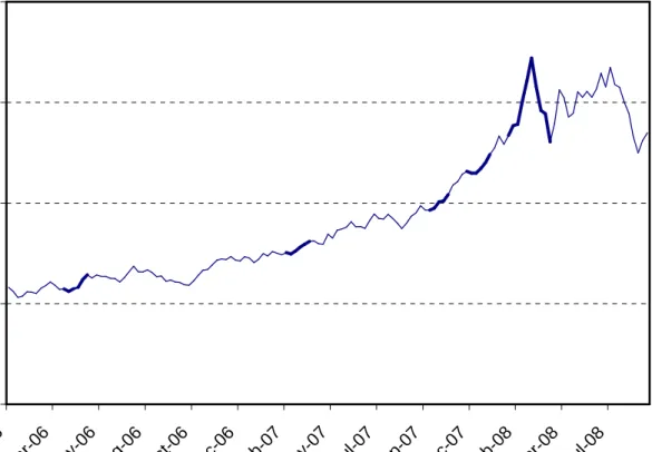
None of this implies that the high food commodity prices over the recent boom were speculative or should be seen as bubbles, or that any bubbles that did occur were necessarily persistent. What they do suggest is that there was some speculative froth, and that this may have contributed to the high prices seen in the markets. Evidence for this may be seen from a plot of the soybean oil price – see Figure 6 where periods in which expectations have been identified as extrapolative are graphed with a heavy line. The chart strongly suggests a speculative bubble in February-March 2008, a time at which industry commentators remarked that prices were out of line with fundamentals.11 However, this bubble was short-lived and the figure does not suggest bubbles in other periods in which prices appear to have been generated extrapolatively.

Speculation is only half of the futures story. The traditional discussion of commodity futures activity has been in terms of hedgers and speculators. However, a new class of transactors in commodity futures markets has become important over the past two decades. These are investors who regard commodity futures as an “asset class”, comparable to equities, bonds, real estate and emerging market assets, and who take positions on commodities as a group

10

An alternative would be to take each commodity-moth pair as a separate observation, the proportion six out of a total of 96 such pairs is in line with a 5% Type I error.

11

For example, in an article dated 18 March 2008 entitled “Focus on soybean oil”, Poultyrsite.com wrote, “… the extreme prices reached in recent weeks exceed levels that might have occurred historically under similar fundamental conditions”. The article concluded “Soybean oil prices appear to remain overvalued …”. http://www.thepoultysite.com/poultrynews/14395/weekly-outlook-focus-on-soybean-oil

based on the risk-return properties of portfolios containing commodity futures relative to those confined to traditional asset classes. Masters (2008) testified before a U.S. Senate committee that the behaviour of this group of transactors is quite different from that of traditional speculators, and it is therefore possible that this will result in different effects on market prices. Gilbert (2009) discusses the differences between futures speculators and futures investors and attempts to quantify the relative importance of each group.

0 20 40 60 80 Ja n-06 Mar -06 May -06 Aug -06 Oct -06 Dec -06 Fe b-07 May -07 Jul-0 7 Sep -07 Dec -07 Fe b-08 Apr -08 Jul-0 8 c /l b

Figure 6: Chicago Board of Trade soybean oil price, January 2006-August 200812

Commodity investors do not generally invest directly in commodity futures, Instead, banks and other financial institutions facilitate such investments by providing suitable instruments, typically Exchange Trade Funds (ETFs), commodity certificates or swaps. In the case of certificates and swaps, they offset much of their net position by taking opposite positions on the futures markets. The majority of such institutions will aim set to replicate a particular

12

commodity futures index in the same way that equity tracking funds aim to replicate the returns on an equities index. Such institutions are referred to as Index Funds.

The most widely followed commodity futures indices are the S&P GSCI and the DJ-AIG Index. The S&P GSCI is weighted in relation to world production of the commodity averaged over the previous five years.13 These are quantity weights and hence imply that the higher the price of the commodity future, the greater its share in the S&P GSCI. Current and recent high energy prices imply a very large energy weighting – 71% in September 2008. The DJ-AIG Index weights the different commodities primarily in terms of the liquidity of the futures contracts (i.e. futures volume and open interest), but in addition considers production. Averaging is again over five years. Importantly, the DJ-AIG Index also aims for diversification and limits the share of any one commodity group to one third of the total. The September 2008 energy share falls just short of this limit.14 September 2008 weightings of these two indices are charted in Figure 7. Agricultural futures comprised 16% of the S&P GSCI and 37% of the DJ-AIG Index.

.

Figure 7: Commodity Composition, S&P GSCI (left) and DJ-AIG Commodity Indices, September 2008

The behaviour of commodity investors differs from that of speculators in three important respects:

13

http://www2.goldmansachs.com/gsci/#passive “Softs” are tropical agricultural commodities or which the most important are cocoa, coffee and sugar.

14 _{http://www.djindexes.com/mdsidx/index.cfm?event=showAigIntro} Energy, 75.6% Precious metals, 1.8% Softs, 2.6% Non-ferrous metals, 6.5% Livestock, 3.5% Grains & vegetable oils, 9.9% Energy, 33.0% Non-ferrous metals, 20.0% Precious metals, 10.1% Softs, 8.7% Livestock, 7.4% Grains & vegetable oils, 20.8%

a) Investors take position across the entire range of commodity futures, not in specific futures

b) Investors are almost always long only while speculators may equally be long or short. c) Investors hold their commodity positions for long periods of time – months or years –

rolling positions forward from expiring to more distant months, while speculators hold positions for short periods of time – days or weeks – and very seldom roll.

According to many commentators, these positions are sufficiently large that index-based inventors have come to dominate the commodity futures markets relegating fundamental factors to a minor, supporting, role. Commodity index providers had invested a total of $43bn in U.S. agricultural futures at the end of 2007, rising to $58bn by the end of June 2008 (CFTC, 2008). This is shown in Table 5 which also gives the shares of the index funds’ net positions in total open interest. These are generally in the 25%-35% range, although higher for wheat, live cattle and lean hogs. They average 27%. In June 2008 testimony before a U.S. Senate committee, Soros (2008) asserted that investment in instruments linked to commodity indices had become the “elephant in the room” and argued that investment in commodity futures might exaggerate price rises.

Table 5

Index Fund Values and Shares U.S. Agricultural Markets

31 Dec 2007 30 June 2008 $bn Share $bn Share Corn 7.6 25.8% 13.1 27.4% Soybeans 8.7 26.1% 10.9 20.8% Soybean oil 2.1 24.8% 2.6 21.7% Wheat 9.3 38.2% 9.7 41.9% Cocoa 0.4 11.3% 0.8 14.1% Coffee 2.2 26.0% 3.1 25.6% Cotton 2.6 33.0% 2.9 21.5% Sugar 3.2 29.0% 4.9 31.1% Feeder cattle 0.4 23.2% 0.6 30.7% Live cattle 4.5 48.4% 6.5 41.8% Lean hogs 2.1 43.6% 3.2 40.6% Total 43.1 26.9% 58.3 27.1%

Source: CFTC (2008) valued at front position closing prices. The wheat figures aggregate positions on the Chicago Board of Trade and the Kansas City Board of Trade. Total shares are price-weighted.

This argument may have force than is often allowed. First, investments are in the entire commodity class, they may be largely independent of current or expected future price movements in specific markets. Secondly, whereas speculators, who rapidly move in and out of markets, provide the liquidity which allows hedgers to obtain counterparties, investors tend to absorb market liquidity, effectively obliging the speculative community to do more work – see Masters (2008). One might paraphrase his view as stating that, in effect, the funds have become the fundamentals.

If these views are correct, we might expect to see commodity price effects from index-based investment, particularly in the less liquid agricultural markets. These effects might include upward pressure on prices, increased price volatility (as the result of reduced market liquidity) and higher correlations across markets. Because index-based investment is still a relatively recent development, empirical evidence remains sparse. We may investigate these links using Granger non-causality analysis, as in section 3. Using information if the CFTC’s Commitments

of Traders supplementary reports, which distinguish positions held by index-providers for twelve

U.S. agricultural futures contracts, I consider the Autoregressive Distributed Lag (ADL) model

3 3 3 0 1 0 0 t j t j j t j j t j t j j j r r₋ x₋ z₋ = = = = α +

∑

∑

∑

where rt is the week-on-week change in the price of the nearby contract, xt is the weekly change

in futures positions of index providers and zt is the weekly change in futures positions of other

non-commercial traders. The equation was estimated by OLS over the sample of weekly data from 31 January 2007 to 26 August 2008 for the four CBOT agricultural futures: corn, soybeans, soybean oil and wheat. In each case, I test six null hypotheses

i) Index positions do not Granger-cause returns: H₀1:β = β = β =_{1 2 3} 0;

ii) Non-commercial positions do not Granger-cause returns: H₀2:γ = γ = γ =_{1 2 3} 0;

iii) Neither index positions nor non-commercial position Granger-cause returns:

3

0 : 1 2 3 1 2 3 0

H β = β = β = γ = γ = γ = ;

iv) Index and non-commercial positions have identical effects on returns:

(

)

4

0 : j j 0,..,3

v) The effects of index positions on returns are non-persistent: 3 5 0 0 : _j 0 j H = β =

∑

vi) The effects of non-commercial positions on returns are non-persistent: 3 6 0 0 : _j 0 j H = γ =

∑

Hypothesis H is interesting only if at least one of ₀4 H ,₀1 H and ₀2 H is rejected, hypothesis ₀3 H is ₀5

interesting only if H is rejected and hypothesis 01 6 0

H is interesting only if H is rejected. 02

Test results are given in Table 6. The tests fail to establish a causal link from either index or non-commercial positions to returns for corn, soybean oil or wheat. By contrast, for soybeans, the hypothesis H that index positions do not Granger-cause soybean returns is rejected. 1₀

Furthermore, the effect, which is estimated as positive, is seen as persistent (H is also rejected). ₀5

The data narrowly fail to reject the Masters (2008) hypothesis,H , that index and speculative ₀4

positions have different effects at the 95% level. These results provide some statistical support for the view that commodity investment contributed to the boom in agricultural food prices.

Table 6

Granger Non-causality Tests

1 0 H H ₀2 H ₀3 H ₀4 H ₀5 H ₀6 3,125 F F3,125 F6,125 F3,125 F1,125 F1,125 Corn 0.50 [68.2%] 0.23 [87.1%] 0.34 [91.4%] 0.53 [66.3%] 0.35 [55.4%] 0.06 [80.0%] Soybeans 3.53 [1.7%] 1.22 [30.6%] 2.07 [6.1%] 2.13 [6.0%] 10.35 [0.2%] 3.51 [6.4%] Soybean Oil 1.91 [13.2%] 0.17 [91.5%] 0.95 [4.61%] 1.76 [16.8%] 1.09 [29.9%] 0.12 [73.3%] Wheat (CBOT) 0.52 [67.2%] 1.27 [28.9%] 0.88 [51.3%] 0.53 [66.3%] 0.10 [74.4%] 1.60 [20.8%] The equation is 3 3 3 0 1 0 0 t j t j j t j j t j t j j j r r₋ x₋ z₋ = = =

= α +

∑

∑

∑

in the price of the nearby contract on the Chicago Board of Trade, xt is the weekly change in

futures positions of index providers and zt is the weekly change in futures positions of other

non-commercial traders. The equation was estimated by OLS over the sample 31 January 2007,

weekly, to 26 August 2008. The null hypotheses are

1 2 3 0: 0 ... 3 0, 0 : 0 ... 3 0, 0 : 0 ... 3 0 ... 3 0 H β = = β = H γ = = γ = H β = = β = γ = = γ = ,

(

)

∑

∑

The two polar positions on the effects of futures market activity on agricultural prices both appear too simple. On the one hand, the efficient markets view that transactions which do not convey information can have no price impact is contradicted by both market experience and econometric evidence. On the other hand, purely speculative episodes, in which price movements become self-reinforcing, tend to be of short duration. Although discussion tends to focus on speculation, it is investment flows that may have resulted in the most marked effects on food prices. The size of these flows can be large relative to overall market capitalization and liquidity. Since commodity investors tend to look at the likely returns to commodities as a class, and not at likely returns on specific markets, their activities may tend to transmit upward (or downward) movements in one market across the entire range of commodity futures markets. This is likely to have resulted in upward pressure in the less liquid agricultural markets and to increased price correlation across markets. It may also have transmitted upward price movements in energy and metals markets into the agricultural commodities.

8. Conclusions

Discussions of the causes of commodity prices tend to adopt an additive framework in which the total impact is the sum of price responses to a set of demand and supply shocks in the underlying markets. This approach may not be helpful in analyzing major booms, such as those of 1972-74 and 2005-08, in which a large number of prices rise together. These additive explanations require too much coincidence and the resulting price responses to shocks may seem disproportionate.

In this paper, I have stressed two factors which can explain the failures of the market-based approach. Firstly, when demand shocks simultaneously impact a number of markets, supply elasticities will tend to be lower than when shocks are market-specific. Secondly, the supply elasticities themselves may depend on macroeconomic and financial factors. The first consideration implies that the behaviour of markets in boom episodes is likely to be different from behaviour under normal conditions. The second implies a likely multiplicative interaction of macroeconomic and financial factors with market shocks which will undermine the additive analysis. Aggregation across a range of markets may imply that these macroeconomic and financial factors are seen as the main determinants of changes in overall prices. In line with this