Methods for Estimation of
Voltage Harmonic Components
Tomáš Radil
1and Pedro M. Ramos
2 1Instituto de Telecomunições, Lisbon
2Instituto de Telecomunições and Department of Electrical and Computer Engineering,
IST, Technical University of Lisbon, Lisbon
Portugal
1. Introduction
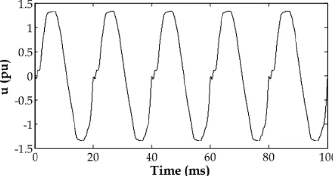
The estimation of harmonic components of power voltage signals is one of the measurements prescribed by the power quality (PQ) standards (IEC 61000-4-30, 2008). In general, the harmonic components originate from non-linear elements connected to the power system such as non-linear loads (e.g., switched-mode power supplies) or transformers. An example of a distorted voltage measured in an office building is shown in Fig. 1. The negative effects associated with the presence of voltage harmonics include, for example, overheating and increased losses of transformers, malfunction of electronic instruments, additional losses in rotating machines or overheating of capacitor banks.
0 20 40 60 80 100 -1.5 -1 -0.5 0 0.5 1 1.5 Time (ms) u ( p u )
Fig. 1. Example of a power voltage distorted by the presence of non-linear loads
The aim of this chapter is to provide an overview of power quality standards related to voltage harmonics assessment and a detailed description of both common and alternative measurement methods.
In this chapter’s introductory part (Section 2), an overview of international standards that concern measurement methods for estimation of voltage harmonics as well as the standards that address the measurement uncertainty limits is provided. This is followed by a description of several applicable measurement methods. The description is divided in two parts: Section 3 deals with methods working in the frequency domain (including the
standard method described in the standard (IEC 61000-4-7, 2009)) while Section 4 contains the description of several time-domain based methods. Each section presents a detailed description of the respective method including its strong and weak points and potential limitations. Section 5 focuses on the calculation of the total harmonic distortion. In Section 6, the performance of the methods described in Section 3 and Section 4 is discussed. The chapter is concluded by Section 7, in which the characteristics of the described algorithms will be summarized.
2. Power quality standards and harmonic estimation
Several international standards deal with the issue of harmonic estimation. In this section, a short overview of these standards and of the requirements imposed in them is provided. In the standard (IEEE 1159-2009, 2009), the harmonics are classified as one of the waveform distortions that typically have a steady state nature, their frequency band is from 0 Hz up to 9 kHz and their magnitude can reach up to 20% of the fundamental.
The standard (IEC 61000–4–7, 2009) describes a general instrument for harmonic estimation. The instrument is based on the Discrete Fourier Transform (DFT); however, the application of other algorithms is also allowed. The DFT algorithm and its application according to the standard are described in Section 3.1. In the standard (IEC 61000–4–30, 2008), it is required that at least 50 harmonics are estimated.
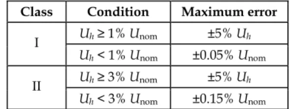
Standard (IEC 61000–4–7, 2009) also includes the accuracy requirements for harmonic estimation. The requirements are divided into two classes: Class I of the IEC 61000–4–7 corresponds to Class A of IEC 61000–4–30, while Class II of the IEC 61000–4–7 corresponds to Class S of IEC 61000–4–30. The requirements are based on the relation between the magnitudes of the measured harmonics (Uh) and the nominal voltage range (Unom) as shown in Table 1.
Class Condition Maximum error
Uh≥ 1% Unom ±5% Uh I Uh < 1% Unom ±0.05% Unom Uh≥ 3% Unom ±5% Uh II Uh < 3% Unom ±0.15% Unom
Table 1. Accuracy requirements for voltage harmonics measurement
The measuring range is specified in (IEC 61000–4–30, 2008) using the compatibility levels (maximum disturbance levels to which a device is likely to be subjected) for low-frequency disturbances in industrial plants, which are standardized in (IEC 61000–2–4, 2002). The measuring range should be from 10% to 200% of the class 3 compatibility levels specified in (IEC 61000–2–4, 2002) for Class A instruments and as 10% to 100% of these compatibility levels for Class S instruments.
The class 3 compatibility levels according to (IEC 61000–2–4, 2002) are shown in Table 2. Note that the compatibility levels of odd harmonics are higher than the compatibility levels of even harmonics. This reflects the fact that in power systems, the odd harmonics are usually dominant.
Harmonic order h Class 3 compatibility level % of fundamental 2 3 3 6 4 1.5 5 8 6 1 7 7 8 1 9 2.5 10 1 11 5 13 4.5 15 2 17 4 21 1.75 10 < h≤ 50 (h even) 1
21 < h≤ 45 (h odd multiples of three) 1 17 < h≤ 49 (h odd) 4.5·(17/h) – 0.5 Table 2. Voltage harmonics compatibility levels
3. Frequency domain methods
One approach to harmonic estimation is to use some kind of a transform to decompose the time series of measured voltage signal samples into frequency components. Most commonly, methods based on the Discrete Fourier Transform (DFT) are used but, for example, the Discrete Wavelet Transform (DWT) is also sometimes applied as well (Pham & Wong, 1999), (Gaouda et al., 2002).
In Section 3.1, the application of the DFT for harmonic estimation according to the standard (IEC 61000-4-7, 2009) is described. In Section 3.2, an alternative method based on the Goertzel algorithm (Goertzel, 1958) and its properties are described.
3.1 Discrete Fourier Transform
The Discrete Fourier Transform (DFT) and its optimized implementation called the Fast Fourier Transform (FFT) is arguably the most used method for harmonic estimation. The harmonic measuring instrument described in (IEC 61000–4–7, 2009) is based on this method. The DFT of a voltage signal u whose length is N samples is described as (Oppenheim et al., 1999) 1 2 / 0 0, , 1 . N ikn N n X k −u n e−π k N = = = … − ⎡ ⎤ ⎡ ⎤ ⎣ ⎦
∑
⎣ ⎦ (1)The result of (1) is a complex frequency spectrum X k⎡ ⎤⎣ ⎦ with frequency resolution of /
S
f f N
where fs is the sampling frequency.
The amplitudes of individual frequency components are then calculated as
( )
2( )
2 2 U k Re X k Im X k N = + ⎡ ⎤ ⎡ ⎤ ⎡ ⎤ ⎣ ⎦ ⎣ ⎦ ⎣ ⎦ (3)In (3), the factor 1 /N is a normalization factor and the multiplication by two is used to take into account the symmetry of a real-input DFT ( X k[ ]= X N[ −k]).
In (IEC 61000–4–7, 2009), the DFT is applied to 10 cycles (in case of 50 Hz power systems) or 12 cycles (in case of 60 Hz power systems) of the power system’s fundamental frequency. Since the power system’s frequency is varying, the length of the window to which the DFT is applied has to be adjusted accordingly. Standard (IEC 61000–4–7, 2009) allows a maximum error of this adjustment of ±0.03%. The window adjustment can be done e.g., by using a phase-locked loop (PLL) to generate the sampling frequency based on the actual power system’s frequency. Alternatively, when the sampling frequency is high enough, the window can be adjusted by selecting the number of samples that correspond to 10 (or 12) cycles at the measured fundamental frequency. In a 50-Hz system, at least fs≅10 kS/s are required to ensure the 0.03% maximum error specification.
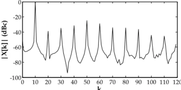
An example of an amplitude DFT spectrum calculated from 10 cycles of the signal shown in Fig. 1 is depicted in Fig. 2.
0 10 20 30 40 50 60 70 80 90 100 110 120 -100 -80 -60 -40 -20 0 k | X [k ]| (d B c)
Fig. 2. Detail of an amplitude DFT spectrum of a measured power voltage signal
Note that when processing signals according to the (IEC 61000–4–7, 2009), the frequency resolution of the spectrum is 5 Hz for both 50 Hz and 60 Hz power systems. This means that the harmonic components (the fundamental, the 2nd and the higher harmonics) can be found
on indices k=10, 20, 30,… for 50 Hz power systems (i.e., U1=U[10], U2=U[20], etc.) and
on 12,k= 24, 36,… for 60 Hz power systems. 3.2 The Goertzel algorithm
The Goertzel algorithm (Goertzel, 1958) is an efficient algorithm for calculation of individual lines of the DFT spectrum. The algorithm applies a second-order infinite impulse response (IIR) filter to the samples of the voltage signal in order to calculate one spectrum line. The Goertzel algorithm calculates the line k of the spectrum using
2 /
[ ] e k N [ – 1] – [ – 2]
X k = π s N s N (4)
[ ] [ ] 2 cos(2 / ) [ 1] – [ – 2]
s n = u n + πk N s n− s n , (5)
[ 1] [ 2] 0
s− = − =s , [ ]u n is the measured voltage signal, N is the number of samples being processed and n∈[0;N−1].
The Goertzel algorithm is more efficient than the Fast Fourier Transform (FFT) when the number of spectrum lines to be calculated (H) meets the condition
2
log ( )
H ≤ N . (6)
However, even when the number of spectrum lines to be calculated does not fulfill the condition (6), the application of the Goertzel algorithm can be advantageous in some cases. It is faster than implementing DFT according to its definition (1) and unlike most of the implementations of the FFT, the Goertzel algorithm does not require N to be an integer power of two. Although algorithms for fast calculation of DFT when the number of samples is not equal to power of two exist, e.g. (Rader, 1968), many libraries for digital signal processing include only the radix-2 FFT. For the Goertzel algorithm, it is sufficient to ensure that N contains an integer number of fundamental periods (to avoid problems with spectrum leakage).
4. Time domain methods
Section 3 described methods for estimation of voltage harmonics in the frequency domain. However, it is possible to estimate the harmonics in the time domain as well. The time-domain approaches are based on a least-square fitting procedure that attempts to estimate the parameters of the voltage signal’s model so the root-mean-square error between the model and the measured signal is minimized.
The time domain methods that try to fit one or more single-tone harmonic signals on the measured signal are in general called sine fitting algorithms.
The general model of a signal that contains multiple harmonic components can be written as
(
)
1 cos 2 H h h h h u U πf t φ C = ⎡ ⎤ =∑
⎣ + ⎦+ (7)where Uh are the amplitudes of individual harmonics, fh their frequencies (expressed as an integer multiple of the fundamental’s frequency: fh= ⋅h f1), ϕh their phases, C is the dc component and H is the number of harmonics included in the model.
For the purpose of the sine fitting algorithms, it is convenient to re-write (7) as
(
)
(
)
1 cos 2 sin 2 H h h h h h u A πf t B πf t C = ⎡ ⎤ =∑
⎣ + ⎦+ (8)where Ah are the in-phase and Bh are the quadrature components. The amplitudes Uh and phases ϕh can be then calculated as
2 2 h h h U = A +B , (9)
(
)
atan2 ; h B Ah h ϕ = − . (10)4.1 The 3- and 4-parameter sine fitting algorithm
The 3- and 4-parameter sine fitting algorithms are described in (IEEE Std. 1057-2007, 2008) where they are used for testing of analog to digital converters in waveform recorders. The 3-parameter algorithm estimates the amplitude and the phase of a signal whose frequency is known. With the frequency known, model (8) is a linear function of the remaining unknown parameters. Thus, the calculation using the 3-parameter sine fitting algorithm is non-iterative and is based on solving
( )
1T T T
A B C = −
⎡ ⎤
⎣ ⎦ D D D u (11)
where u is the column vector of measured voltage samples, D is a matrix
(
)
(
)
(
)
(
)
(
)
(
)
0 0 1 1 1 1 cos 2 sin 2 1 cos 2 sin 2 1 cos 2 N sin 2 N 1 ft ft ft ft ft ft π π π π π − π − ⎡ ⎤ ⎢ ⎥ ⎢ ⎥ = ⎢ ⎥ ⎢ ⎥ ⎢ ⎥ ⎣ ⎦ D B B B (12)and tn are the timestamps of voltage samples.
The accuracy of the 3-parameter sine fitting algorithm depends on the frequency estimate. The frequency can be estimated using algorithms such as the Interpolated DFT (IpDFT) algorithm (Renders et al., 1984); however, many algorithms are applicable for this task (Slepička et al., 2010).
In case the frequency estimate is not sufficiently accurate (Andersson & Händle, 2006), the 4-parameter algorithm can be used. Including the frequency in the algorithm makes the least-square procedure non-linear, which means that the algorithm has to use an iterative optimization process to find the optimum value of the estimated parameters.
The 4-parameter sine fitting algorithm solves the equation
( ) ( ) ( ) ( ) T
( )
( ) T ( ) 1 ( ) T Δ i i i i i i i A B C ω − ⎡ ⎤ ⎡ ⎤ = ⎢ ⎥ ⎡ ⎤ ⎣ ⎦ ⎣ D D ⎦ ⎣D ⎦ u (13)where i is the iteration number, ω is the angular frequency ω=2πf ; Δω( )i is the change of the angular frequency from the previous iteration, matrix D(i) is
( ) ( )
(
)
(
( ))
( )( )
( )(
)
(
( ))
( )( )
( )(
)
(
( ))
( )(
)
1 1 1 0 0 0 1 1 1 1 1 1 1 1 1 1 1 1 cos sin 1 cos sin 1 cos sin 1 i i i i i i i i i i N N N t t t t t t t t t ω ω α ω ω α ω ω α − − − − − − − − − − − − ⎡ ⎤ ⎢ ⎥ ⎢ ⎥ ⎢ ⎥ = ⎢ ⎥ ⎢ ⎥ ⎢ ⎥ ⎢ ⎥ ⎣ ⎦ D B B B B , (14)and α( )i−1
( )
t = −A( )i−1t×sin( )
ω( )i−1t +B( )i−1t×cos( )
ω( )i−1t .The iterative computation continues until the absolute relative change of the estimated frequency drops below a predefined threshold or until the maximum number of allowed iterations is exceeded.
In order to estimate the voltage harmonics, first, the 4-parameter sine fitting algorithm is applied to the voltage signal and the signal’s fundamental frequency, amplitude and phase are estimated. In the second step, the 3-parameter algorithm is repeatedly applied to the residuals after estimation of the fundamental to estimate the individual higher harmonics. This means that the frequency supplied to the 3-paramater algorithm is an integer multiple of the fundamental’s estimated frequency.
4.2 The multiharmonic fitting algorithm
The previously described combination of the 4- and 3-parameter sine fitting algorithms estimates the harmonic amplitudes and phases one by one. The advantage of this approach is that it keeps the computational requirements low because in each step only operations with small matrices are required. Its weak point is that it relies on the accuracy of the estimation of the fundamental frequency using the 4-paramater algorithm. Since the 3- and 4-parameter algorithms take into account only one frequency at a time, the other frequencies contained in the signal act as disturbances that affect the final estimate of the frequency and of the harmonic amplitudes.
The multiharmonic fitting algorithm (Ramos et al., 2006) provides more accurate but also computationally heavier approach. It uses an optimization procedure in which all the parameters (i.e., the fundamental’s frequency and the amplitudes and phases of all harmonics) are estimated at the same time.
There are two versions of the multiharmonic fitting algorithm: non-iterative and iterative version.
The non-iterative version is similar to the 3-parameter sine fitting algorithm. It assumes that the signal’s fundamental frequency is known and estimates the remaining parameters (the components Ah and Bh of the harmonic amplitudes and the dc component C)
( )
1 T T T 1 1 2 2 H H A B A B A B C = − ⎡ ⎤ ⎣ A ⎦ D D D u (15) where D is a matrix( )
( )
( )
( )
(
)
(
)
( )
( )
( )
( )
(
)
(
)
(
)
(
)
(
)
(
)
(
)
(
)
0 0 0 0 0 0 1 1 1 1 1 1 1 1 1 1 1 1cos sin cos 2 sin 2 cos sin 1
cos sin cos 2 sin 2 cos sin 1
cos N sin N cos 2 N sin 2 N cos N sin N 1
t t t t H t H t t t t t H t H t t t t t H t H t ω ω ω ω ω ω ω ω ω ω ω ω ω − ω − ω − ω − ω − ω − ⎡ ⎤ ⎢ ⎥ ⎢ ⎥ = ⎢ ⎥ ⎢ ⎥ ⎢ ⎥ ⎣ ⎦ D A A B B B B D B B B A (16)
and ω is the angular frequency of the fundamental.
As in the case of the 3-parameter sine fitting algorithm, the non-iterative multiharmonic algorithm relies on the initial frequency estimate. However, the initial estimate can be improved using an iterative optimization procedure.
The iterative multiharmonic fitting algorithm adds the frequency into the calculations
( ) ( ) ( ) ( ) ( ) ( ) ( ) ( ) T
( )
( ) T ( ) 1 ( ) T 1 1 1 2 2 Δ i i i i i i i i i i i H H A B A B A B C ω − − ⎡ ⎤ ⎡ ⎤ = ⎢ ⎥ ⎡ ⎤ ⎢ ⎥ ⎣ ⎦ ⎣ A ⎦ ⎣ D D ⎦ D u (17) where ( )i D is a matrix( )
( )
( )
(
)
(
)
( )( )
( )
( )
(
)
(
)
( )( )
(
)
(
)
(
)
(
)
( )(
)
1 0 0 0 0 0 1 1 1 1 1 1 1 1 1 1 1 1cos sin cos sin 1
cos sin cos sin 1
cos sin cos sin 1
i i i i N N N N N t t H t H t t t t H t H t t t t H t H t t ω ω ω ω α ω ω ω ω α ω ω ω ω α − − − − − − − − ⎡ ⎤ ⎢ ⎥ ⎢ ⎥ = ⎢ ⎥ ⎢ ⎥ ⎢ ⎥ ⎢ ⎥ ⎣ ⎦ D A A B B D B B B B A (18) and ( )1
( )
( )1(
( )1)
( )1(
( )1)
1 sin cos H i i i i i h h h t A ht h t B ht h t α − − ω − − ω − = ⎡ ⎤ = ⎢− + ⎥ ⎣ ⎦∑
.5. Calculation of the Total Harmonic Distortion
The Total Harmonic Distortion (THD) is an important indicator used to express the total amount of harmonic components. It is defined as
2 2 1 H h h U THD U = =
∑
(19)and expressed in relative units or in percents.
For stationary signals whose length is exactly 10 cycles (or 12 in case of 60 Hz power systems) the whole energy of a harmonic component is concentrated in one frequency bin. However, if the signal’s parameters such as its fundamental frequency vary, the energy will leak into neighbouring frequency bins (spectral leakage). To take into account this effect, the standard (IEC 61000-4-7, 2009) defines, besides the THD, two more indicators: the group total harmonic distortion (THDG) and the subgroup total harmonic distortion (THDS). The group total harmonic distortion is defined as
2 , 2 ,1 H g h h g U THDG U = =
∑
(20) where 1 2 2 2 2 2 , 1 2 1 1 2 2 2 2 P g h P k P P U U P h U P h k U P h − =− + ⎡ ⎤ ⎡ ⎤ = ⎣ ⋅ − ⎦+∑
⎡⎣ ⋅ − +⎤⎦ ⎣ ⋅ + ⎦ (21) and P is the number of fundamental periods within the signal (P=10 for 50 Hz powersystems and P=12 for 60 Hz power systems). The subgroup total harmonic distortion is defined as
2 , 2 ,1 H sg h h sg U THDS U = =
∑
(22) where 1 2 2 , 1 . sg h k U U P h k =− =∑
⎡⎣ ⋅ + ⎤⎦ (23)Note that only the THD can be calculated when using the time-domain fitting algorithms. The Goertzel algorithm is not suitable when THDG and THDS have to be estimated, because as the number of spectrum lines that have to be calculated increases, the algorithm’s computational requirements also increase significantly.
6. Comparison of the methods
In this section, the above described methods for harmonics estimation are compared. Their accuracy is discussed in Section 6.1, while Section 6.2 focuses on the computational requirements of individual algorithms.
6.1 Accuracy
The standard (IEC 61000-4-30, 2008) specifies the conditions under which power quality measuring instruments should be tested. The standard recognizes three classes of instruments: Class A, Class S and Class B instruments. While for classes A and S the tests and required performance is described in the standard, the performance of Class B instruments is specified by manufacturer.
As it was described in Section 2 of this chapter, the levels of harmonics in signals used for testing should be up to 200% of the values in Table 1 for Class A instruments and 100% of these values for Class S instruments. Furthermore, the test signals should contain other disturbances and variations of parameters as described by the three testing states. The most important parameters of these testing states are summarized in Table 3.
Influence
quantity Testing state 1 Testing state 2 Testing state 3 Frequency fnom ± 0.5 Hz fnom – 1 Hz ± 0.5 Hz fnom + 1 Hz ± 0.5 Hz
Flicker Pst < 0.1 Pst = 1 ± 0.1 Pst = 4 ± 0.1 Voltage Udin ± 1% determined by flicker
and interharmonics
determined by flicker and interharmonics Interharmonics 0% to 0.5% Udin 1% ± 0.5% Udin at 7.5·fnom 1% ± 0.5% Udin at 3.5·fnom Table 3. Testing conditions for Class A and S instruments according to IEC 61000-4-30 In Table 3, fnom designates the nominal power frequency, Pst is the short-term flicker severity and Udin is the nominal input voltage.
Test signals according to the three testing states were simulated in order to test the above described algorithms for harmonic estimation. Harmonics were added to the signals to achieve signals with THD = 20%. The phases of harmonics were random and the distribution of harmonic amplitudes was as follows from Table 4.
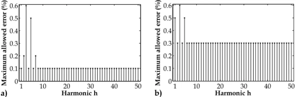
The testing signals also contained white Gaussian noise corresponding to a signal to noise ratio of 75 dB (the noise was added to simulate the equivalent noise of an ideal 12-bit analog to digital converter). The Goertzel algorithm, the combined 4- and 3- parameter sine fitting algorithm, the non-iterative multiharmonic fitting and the iterative multiharmonic fitting algorithm were applied to 10 000 of such test signals and the maximum error of estimation of individual harmonic amplitudes was calculated. The maximum allowed error for individual harmonics calculated using the Table 1 are shown in Fig. 3a and Fig. 3b for Class A and Class S instruments, respectively. The simulation results for the three testing states are shown in Fig. 4, Fig. 5 and Fig. 6.
Harmonic order h Amplitude (in % of the fundamental) 2nd 4% 3rd 12% 4th 2% 5th 10% 7th 4% h odd from 9th to 17th 2% h even from 6th to 18th 1.6% h from 19th to 50th 1.6%
Table 4. Distribution of harmonic amplitudes in the test signals
1 10 20 30 40 50 0 0.1 0.2 0.3 0.4 0.5 0.6 Harmonic h Maxim u m allo wed er ro r (% ) a) 1 10 20 30 40 50 0 0.1 0.2 0.3 0.4 0.5 0.6 Harmonic h M a x im u m a ll o w e d e rr o r ( % ) b)
Fig. 3. Maximum allowed error of harmonic estimation for a) Class A and b) Class S instruments
From the comparison of Fig. 4a, Fig. 5a and Fig. 6a with Fig. 3a it can be seen that the DFT (i.e., also the Goertzel algorithm), the non-iterative multiharmonic fitting and the iterative harmonic fitting are all suitable for a Class A instrument according to the IEC 61000-4-30 specification. The combined 4- and 3-paramter sine fitting algorithm produces worse results. However, this algorithm can still be used in Class S or Class B instruments (compare Fig. 4b, Fig. 5b and Fig. 6b with Fig. 3b). Note that the harmonic levels employed in the test corresponded to Class A testing; for Class S lower levels should be applied (e.g., the THD should be up to 10%).
From Fig. 4a, Fig. 5a and Fig. 6a it can be seen that the multiharmonic algorithms are more accurate than the DFT calculation and that the difference between the results provided by the non-iterative and the iterative multiharmonic algorithm is negligible. The main difference between these two algorithms is in the estimates of the phases and in the frequency estimate, which are not employed when estimating only harmonic amplitudes. In the following test, the accuracy of estimation of the THD was investigated. Signals with THD ranging from 0.5% up to 20% were simulated. The signals contained influencing quantities according to the testing state 3 (see Table 3) and normally distributed additive noise corresponding to the equivalent noise of an ideal 12-bit analog to digital converter. In total, 10 000 of such signals were simulated and the considered algorithms were applied to them. The DFT was used to calculate the values of THD (19), THDG (20) and THDS (22). The maximum absolute errors of estimation of the THD using all the algorithms are shown in Fig. 7.
1 5 10 15 20 25 30 35 40 45 50 0 0.005 0.01 0.015 Harmonic h M ax im u m e rr o r (%
) Non-iterative multiharm. Multiharmonic DFT
a) 1 5 10 15 20 25 30 35 40 45 50 0 0.05 0.1 0.15 0.2 0.25 0.3 Harmonic h M axim u m er ro r (%
) 4- and 3- parameter sine fitting
b)
Fig. 4. Accuracy of estimation of harmonic amplitudes – testing state 1
1 5 10 15 20 25 30 35 40 45 50 0 0.005 0.01 0.015 Harmonic h M axim u m er ro r (%
) Non-iterative multiharm. Multiharmonic DFT
a) 1 5 10 15 20 25 30 35 40 45 50 0 0.05 0.1 0.15 0.2 0.25 0.3 Harmonic h M axim u m er ro r (%
) 4- and 3- parameter sine fitting
b)
1 5 10 15 20 25 30 35 40 45 50 0 0.005 0.01 0.015 Harmonic h M ax im u m e rr o r (%
) Non-iterative multiharm. Multiharmonic DFT
a) 1 5 10 15 20 25 30 35 40 45 50 0 0.05 0.1 0.15 0.2 0.25 0.3 Harmonic h M axim u m er ro r (%
) 4- and 3- parameter sine fitting
b)
Fig. 6. Accuracy of estimation of harmonic amplitudes – testing state 3
The calculation of the THDG values includes all the spectrum lines of the DFT spectrum. This means, that it includes also the frequencies that contain spurious components (e.g., the interharmonic component) and the noise. This explains the poor results of the THDG shown in Fig. 7. The rest of the algorithms produced almost identical results. Only the combined 4- and 3-parameter sine fitting algorithm performs slightly worse for higher values of the THD.
0 0.05 0.1 0.15 0.2 10-4 10-3 10-2 THD (-) Max. e rr o r o f T HD es tim atio n (-) DFT (THD) DFT (THDG) DFT (THDS) 4- and 3-par. sine fitting Non-iterative multiharmonic Multiharmonic
6.2 Computational requirements
In this section, the memory and processing time requirements of the previously described algorithms are discussed.
The memory requirements of the algorithms for fast calculation of the DFT depend on the particular implementation and can differ substantially. For example, the real radix-2 FFT available as a library function in the VisualDSP++ development environment for digital signal processors (Analog Devices, 2010) requires 2 × N memory spaces to store the real and imaginary part of the result and 3 × N/4 memory space to store the twiddle factors.
The Goertzel algorithm has very low memory requirements which do not depend on the number of processed samples N. A typical implementation requires only 4 memory spaces: 2 for the variable s; one for the multiplication constant in (5) and one auxiliary variable. When implementing the 3- and 4-parameter sine fitting algorithms by the definition (see (11) and (13), respectively), it is necessary to construct the matrix D whose size is N×3 and
4
N× , respectively. However, both algorithms can be optimized by constructing directly the resulting matrices D DT and D uT . This way, only matrices 3 3× and 3 1× (in the case 3-parameter sine fitting algorithm) or 4 4× and 4 1× (in the case 4-parameter sine fitting algorithm) have to be stored in the memory. Besides saving memory space, this approach is also faster because some of elements of these matrices are identical (Radil, 2009). This way, the 3-parameter algorithm requires 24 memory spaces and the 4-paramater algorithm requires 40 memory spaces independent of the length of the processed signal. The values include the space for intermediate results and exclude memory space required to calculate the initial estimate.
The multiharmonic fitting algorithms are more complex and attempts to construct the matrices D DT and D uT directly lead to higher computational burden. The non-iterative multiharmonic algorithm requires
(
N+ ×2) (
2H+ + ×1)
2(
2H+1)
2 memory space and the iterative algorithm requires(
N+ ×2) (
2H+ + ×2)
2(
2H+2)
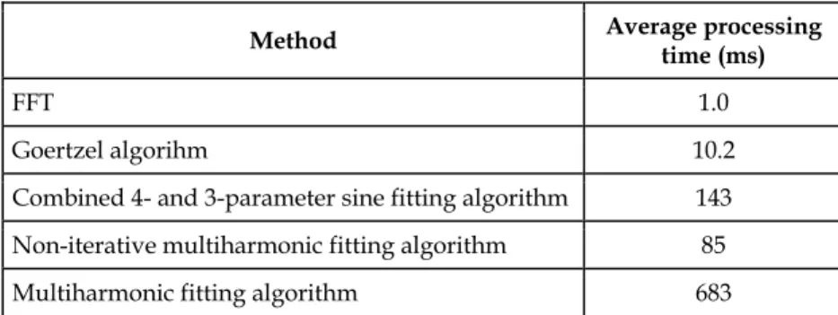
2 (including the space for intermediate results and excluding memory space required to calculate the initial estimate). Another important parameter of methods for estimation of harmonics is their time consumption because in power quality monitoring it is usually required that all the processing, including the harmonic estimation, is performed in real-time.To test the processing time required by individual algorithm, 10 000 signals with frequency 49.95 Hz
f = , 2%THD= and random normally distributed noise were simulated. The signals were 10 fundamental cycles long (10 010 samples at fs=50 kS/s). The average processing time of individual algorithms implemented in Matlab was then evaluated and is shown in Table 5.
From Table 5 it can be seen that, as expected, the FFT is the fastest of the considered algorithms. However, the Goertzel algorithm, the combined 4- and 3-parameter sine fitting algorithm and the non-iterative multiharmonic fitting are also able to work in real-time (the length of the processed signal was approximately 200 ms).
Furthermore, some of the algorithms were implemented in a digital signal processor (DSP) Analog Devices ADSP-21369 running at the clock frequency of 264 MHz. A DSP like this one can be used for real-time processing in a power quality analyzer (Radil, 2009). Only the algorithms, whose implementation fits into the DSP’s internal memory, were selected. The algorithms are: 2048-point FFT, the Goertzel algorithm and the combined 4- and 3- parameter sine fitting algorithm. The DSP was acquiring a voltage signal from a 230 V/50 Hz power system at a sampling rate fs=10kS/s.. The average processing times are shown in Table 6.
The results in Table 6 are similar to the results shown in Table 5 and all three considered algorithms are suitable for real-time operation.
Note that the processing time of the 4-parameter algorithm shown in Table 6 is composed of two parts: initial calculations whose length depends only on the number of samples and the iterative parts which depends on the number of iterations required by the algorithm to converge. In the DSP implementation, the algorithm required on average 3 iterations. Significantly higher number of iterations indicates that the processed signal is disrupted by e.g., sag or interruption.
Method Average processing
time (ms)
FFT 1.0
Goertzel algorihm 10.2
Combined 4- and 3-parameter sine fitting algorithm 143 Non-iterative multiharmonic fitting algorithm 85
Multiharmonic fitting algorithm 683
Table 5. Average processing times of the algorithms implemented in Matlab
Method Average processing
time (ms)
FFT 0.5
Goertzel algorihm 1.53
Combined 4- and 3-parameter sine fitting algorithm 100.2 Table 6. Average processing times of the algorithms implemented in a DSP
7. Summary and conclusions
In this chapter, an overview of several methods applicable for estimation of voltage harmonics was provided. The methods include: DFT, the Goertzel algorithm, method based on the 4- and 3-parameter sine fitting algorithms, the non-iterative multiharmonic fitting and the iterative multiharmonic fitting.
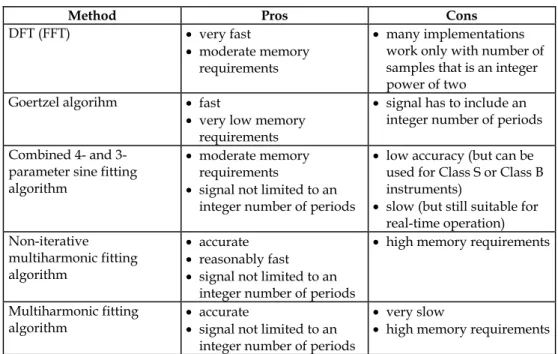
The DFT algorithm is a standard algorithm recommended by the power quality standards. However, as it was shown in Section 6 of this chapter, other methods can provided higher accuracy and/or lower computational and implementation requirements. The summary of the properties of the discussed methods is shown in Table 7. The selection of the most suitable method then depends on the requirements of each application and on the available resources.
Method Pros Cons
DFT (FFT) • very fast
• moderate memory requirements
• many implementations work only with number of samples that is an integer power of two
Goertzel algorihm • fast
• very low memory requirements
• signal has to include an integer number of periods Combined 4- and
3-parameter sine fitting algorithm
• moderate memory requirements
• signal not limited to an integer number of periods
• low accuracy (but can be used for Class S or Class B instruments)
• slow (but still suitable for real-time operation) Non-iterative multiharmonic fitting algorithm • accurate • reasonably fast
• signal not limited to an integer number of periods
• high memory requirements
Multiharmonic fitting
algorithm •
accurate
• signal not limited to an integer number of periods
• very slow
• high memory requirements Table 7. Summary of the properties of the described algorithms for harmonic estimation
8. References
Analog Devices (2010). VisualDSP++ 5.0 Run-Time Library Manual for SHARC Processors (Edition 1.4), Analog Devices, Inc.
Andersson, T.; Händel, P. (2006). IEEE Standard 1057, Cramér-Rao bound and the parsimony principle, IEEE Transactions on Instrumentation and Measurement, vol. 55, no. 1, February 2006, pp. 44 - 53, ISSN 0018-9456
Gaouda, A. M.; Kanoun, S. H.; Salama, M. M. A.; Chikhani, A. Y. (2002). Wavelet-based signal processing for disturbance classification and measurement, IEE Proceedings - Generation, Transmission and Distribution, vol. 149, no. 3, May 2002, pp. 310 – 318, ISSN 1350-2360
Goertzel, G. (1958). An algorithm for the evaluation of finite trigonometric series, The American Mathematical Monthly, vol. 65, no. 1, January 1958, pp. 34 – 35, ISSN 0002-9890
IEC 61000-2-4 (2002). IEC 61000-2-4 Electromagnetic compatibility (EMC) – Part 2-4: Environment – Compatibility levels in industrial plants for low-frequency conducted disturbances, Edition 2.0, IEC, ISBN 2-8318-6413-5
IEC 61000-4-7 (2009). IEC 61000-4-7 Electromagnetic compatibility (EMC) – Part 4-7: Testing and measurement techniques – General guide on harmonics and interharmonics measurements and instrumentation, for power supply systems and equipment connected thereto, Edition 2.1, IEC, ISBN 2-8318-1062-6
IEC 61000-4-30 (2008). IEC 61000-4-30 Electromagnetic compatibility (EMC) – Part 4-30: Testing and measurement techniques – Power quality measurement methods, Edition 2.0, IEC, ISBN 2-8318-1002-0
IEEE Std. 1057-2007 (2008). IEEE Standard for Digitizing Waveform Recorders, IEEE Instrumentation and Measurement Society, ISBN 978-0-7381-5350-6
IEEE Std. 1159-2009 (2009). IEEE Recommended Practice for Monitoring Electric Power Quality, IEEE Power & Energy Society, ISBN 978-0-7381-5939-3
Oppenheim, A. V.; Schafer, R. W.; Buck, J. R. (1999). Discrete-time signal processing. Upper Saddle River, N.J.: Prentice Hall. ISBN 0-13-754920-2
Pham, V.L.; Wong, K.P. (1999). Wavelet-transform-based algorithm for harmonic analysis of power system waveforms, IEE Proceedings on Generation, Transmission and Distribution, vol. 146, no. 3, May 1999, pp. 249-254, ISSN 1350-2360
Rader, C. M. (1968). Discrete Fourier transforms when the number of data samples is prime, Proceedings of the IEEE, vol. 56, no. 6, June 1968, pp. 1107- 1108, ISSN 0018-9219 Radil, T.; Ramos, P. M.; Serra, A. C. (2009). Single-phase power quality analyzer based on a
new detection and classification algorithm, Procedings of IMEKO World Congress, pp. 917 – 922, ISBN 978-963-88410-0-1, Lisbon, Portugal, September 2009
Ramos, P. M.; da Silva, M. F.; Martins, R. C.; Serra, A. C. (2006). Simulation and experimental results of multiharmonic least-squares fitting algorithms applied to periodic signals, IEEE Transactions on Instrumentation and Measurement, vol. 55, no. 2, April 2006, pp. 646 – 651, ISSN 0018-9456
Renders, H.; Schoukens, J.; Vilain, G. (1984). High-Accuracy Spectrum Analysis of Sampled Discrete Frequency Signals by Analytical Leakage Compensation”, IEEE Transactions on Instrumentation and Measurement, vol. 33, no. 4, December 1984, pp. 287 – 292, ISSN 0018-9456
Slepička, D.; Petri, D.; Agrež, D.; Radil, T.; Lapuh, R.; Schoukens, J.; Nunzi, E.; Sedláček, M. (2010). Comparison of Nonparametric Frequency Estimators, Proceedings of the IEEE International Instrumentation and Technology Conf. - I2MTC, pp. 73 – 77, ISBN 978-1-4244-2833-5, Austin, USA, May 2010
Edited by Mr Andreas Eberhard
ISBN 978-953-307-180-0 Hard cover, 362 pages Publisher InTech
Published online 11, April, 2011 Published in print edition April, 2011
InTech Europe
University Campus STeP Ri Slavka Krautzeka 83/A 51000 Rijeka, Croatia Phone: +385 (51) 770 447 Fax: +385 (51) 686 166 www.intechopen.com
InTech China
Unit 405, Office Block, Hotel Equatorial Shanghai No.65, Yan An Road (West), Shanghai, 200040, China Phone: +86-21-62489820
Fax: +86-21-62489821
Almost all experts are in agreement - although we will see an improvement in metering and control of the power flow, Power Quality will suffer. This book will give an overview of how power quality might impact our lives today and tomorrow, introduce new ways to monitor power quality and inform us about interesting possibilities to mitigate power quality problems.
How to reference
In order to correctly reference this scholarly work, feel free to copy and paste the following:
Tomáš Radil and Pedro M. Ramos (2011). Methods for Estimation of Voltage Harmonic Components, Power Quality, Mr Andreas Eberhard (Ed.), ISBN: 978-953-307-180-0, InTech, Available from: