Convergence and stability of the inverse scattering
series for diffuse waves
Shari Moskow
Department of Mathematics, Drexel University, Philadelphia, PA 19104, USA E-mail: [email protected]
John C. Schotland
Department of Bioengineering and Graduate Group in Applied Mathematics and Computational Science, University of Pennsylvania, Philadelphia, PA 19104, USA E-mail: [email protected]
Abstract. We analyze the inverse scattering series for diffuse waves in random media. In previous work the inverse series was used to develop fast, direct image reconstruction algorithms in optical tomography. Here we characterize the convergence, stability and approximation error of the series.
PACS numbers: 42.30.Wb, 41.20.Jb, 42.62.Be
1. Introduction
The inverse scattering problem (ISP) for diffuse waves consists of recovering the spatially-varying absorption of the interior of a bounded domain from measurements taken on its boundary. The problem has been widely studied in the context of optical tomography—an emerging biomedical imaging modality which uses near-infrared light as a probe of tissue structure and function [17, 1]. More generally, diffusion of multiply-scattered waves is a nearly universal feature of wave propagation in random media [19].
The ISP in optical tomography is usually formulated as a nonlinear optimization problem. At present, the iterative methods which are used to solve this problem are not well understood mathematically, since error estimates and convergence results are not known. In this paper we will show that, to some extent, it is possible to fill this gap. In particular, we will study the solution to the ISP which arises from inversion of the Born series. In previous work we have utilized such series expansions as tools to develop fast, direct image reconstruction algorithms [10]. Here we characterize their convergence, stability and reconstruction error.
Early work on series solutions to the quantum-mechanical inverse backscattering problem was carried out by Jost and Kohn [7], Moses [13] and Prosser [16]. There has also been more recent work on the inverse medium problem for acoustic waves [5, 18, 20]. However, it is important to note, that the procedures employed in these papers are purely formal [14].
The remainder of this paper is organized as follows. In Section 2 we develop the scattering theory of diffuse waves in an inhomogeneous medium—this corresponds to the forward problem of optical tomography. We then derive various estimates which are later used to study the convergence of the Born series and its inverse. The inversion of the Born series is taken up in Section 3, where we also obtain our main results on the convergence, stability and approximation error of the inverse series. In Section 4 we discuss numerical applications of our results. Finally, in Section 5 we show that our results extend to the case of the ISP for propagating scalar waves.
2. Forward Problem
Let Ω be a bounded domain in Rn, for n≥2, with a smooth boundary ∂Ω. We consider the propagation of a diffuse wave in an absorbing medium whose energy density u satisfies the time-independent diffusion equation
−∇2u(x) +k2(1 +η(x))u(x) = 0 , x∈Ω, (1) where the diffuse wave number k is a positive constant and η(x) ≥ −1 for all x ∈ Ω. The function η is the spatially varying part of the absorption coefficient which is assumed to be supported in a closed ball Ba of radius a. The energy density is also taken to obey the boundary condition
u(x) +ℓν· ∇u(x) = 0 , x∈∂Ω , (2)
where ν is the unit outward normal to ∂Ω and the extrapolation length ℓ is a nonnegative constant. Note thatk andη are related to the absorption and reduced scattering coefficients
µa and µ′s by k =
√
3¯µaµ′s and η(x) = δµa(x)/µ¯a, where δµa(x) = ¯µa −µa(x) and ¯µa is constant [12].
The forward problem of optical tomography is to determine the energy density u for a given absorption η. If the medium is illuminated by a point source, the solution to the forward problem is given by the integral equation
u(x) = ui(x)−k2
Z
Ω
G(x, y)u(y)η(y)dy , x∈Ω . (3) Hereui is the energy density of the incident diffuse wave which obeys the equation
and G is the Green’s function for the operator −∇2 +k2, where G obeys the boundary condition (2). We may express Gas the sum of the fundamental solution
G0(x, y) = e
−k|x−y|
4π|x−y| , x, y ∈Ω (5)
and a solution to the boundary value problem
−∇2F(x) +k2F(x) = 0 , x∈Ω (6)
F(x) +ℓν· ∇F(x) = −G0(x, y)−ℓν· ∇G0(x, y) , x∈∂Ω ,
for each y ∈Ω. That is, we have G=G0+F. By [6] Theorem 6.31, F ∈C2( ¯Ω) when y is
in the interior of Ω.
The integral equation (3) has a unique solution. If we apply fixed point iteration (beginning with ui), we obtain an infinite series for u of the form
u(x) = ui(x)−k2 Z Ω G(x, y)η(y)ui(y)dy + k4 Z Ω×Ω G(x, y)η(y)G(y, y′)η(y′)ui(y′)dydy′+· · · . (7) We will refer to (7) as the Born series and the approximation touthat results from retaining only the linear term in η as the Born approximation.
It will prove useful to express the Born series as a formal power series in tensor powers of η of the form
φ=K1η+K2η⊗η+K3η⊗η⊗η+· · · , (8)
where φ =ui−u. Physically, the scattering data φ(x1, x2) is proportional to the change in intensity measured by a point detector at x2 ∈ ∂Ω due to a point source at x1 ∈ ∂Ω [10]. Each term in the series is multilinear in η and the operator Kj is defined by
(Kjf) (x1, x2) = (−1)j+1k2j
Z
Ba×···×Ba
G(x1, y1)G(y1, y2)· · ·G(yj−1, yj)G(yj, x2)f(y1, . . . , yj)dy1· · ·dyj , (9) for x1, x2 ∈ ∂Ω. To study the convergence of the series (8) we require an estimate on the L∞ norm of the operator K
j. Let f ∈L∞(Ba× · · · ×Ba). Then kKjfkL∞(∂Ω×∂Ω) = sup (x1,x2)∈∂Ω×∂Ω |(Kjf)(x1, x2)| ≤ kfk∞ sup (x1,x2)∈∂Ω×∂Ω k2j Z Ba×···×Ba |G(x1, y1)· · ·G(yj, x2)|dy1· · ·dyj . (10) We begin by estimating the above integral for j = 1,
kK1k∞≤ sup (x1,x2)∈∂Ω×∂Ω k2 Z Ba |G(x1, y)G(y, x2)|dy ≤k2|Ba|sup x∈Ba sup y∈∂Ω| G(x, y)|2 . (11)
Now, for j ≥2, we take out the first and last factors ofG in the integral to obtain kKjk∞≤ sup (x1,x2)∈∂Ω×∂Ω sup y1∈Ba,yj∈Ba |G(x1, y1)G(yj, x2)| ·k2j Z Ba×···×Ba |G(y1, y2)· · ·G(yj−1, yj)|dy1· · ·dyj . (12) We then rewrite this as
kKjk∞≤ sup x∈Ba sup y∈∂Ω| G(x, y)|2Ij−1 , (13) where Ij−1 =k2j Z Ba×···×Ba |G(y1, y2)· · ·G(yj−1, yj)|dy1· · ·dyj . (14) Next, we estimate Ij−1 recursively:
Ij−1 ≤ sup yj−1∈Ba k2 Z Ba |G(yj−1, yj)|dyj ·k2j−2 Z Ba×···×Ba |G(y1, y2)· · ·G(yj−2, yj−1)|dy1· · ·dyj−1 , (15)
from which it follows that
Ij−1 ≤µ∞Ij−2 , (16) where µ∞ = sup x∈Ba k2kG(x,·)kL1 (Ba) . (17)
We also note that
I1 =k4 Z Ba×Ba |G(x, y)|dxdy (18) ≤k2|Ba|µ∞. Thus Ij−1 ≤k2|Ba|µj∞−1 . (19) Define ν∞ =k2|Ba| sup x∈Ba sup y∈∂Ω| G(x, y)|2 . (20)
Note that the smoothness of solutions to (6) implies that µ∞ and ν∞ are bounded. Making
use of (12) and (19) we obtain the following lemma.
Lemma 2.1. The operator
Kj :L∞(Ba× · · · ×Ba)−→L∞(∂Ω×∂Ω)
defined by (9) is bounded and
kKjk∞≤ν∞µj∞−1 ,
We now obtain similar L2 estimates on the norm of Kj. Let f ∈ L2(Ba× · · · ×Ba). Then kKjfk2L2(∂Ω×∂Ω) = Z ∂Ω×∂Ω| (Kjf)(x1, x2)|2dx1dx2 . (21) From (9) and the Cauchy-Schwarz inequality we have
|(Kjf)(x1, x2)| ≤k2jkfkL2 Z Ba×···×Ba |G(x1, y1)G(y1, y2)· · ·G(yj, x2)|2dy1· · ·dyj 1/2 . (22) We begin by estimating kK1k: kK1k2 ≤k2 Z ∂Ω×∂Ω Z Ba |G(x1, y)G(y, x2)|2dx1dx2dy 1/2 ≤k2|Ba|1/2 sup x∈Ba kG(x,·)k2L2(∂Ω) . (23)
Now, for j ≥2, we find that
kKjk22 ≤ sup y1∈Ba,yj∈Ba Z ∂Ω×∂Ω| G(x1, y1)G(x2, yj)|2dx1dx2 ·k4j Z Ba×···×Ba |G(y1, y2)· · ·G(yj−1, yj)|2dy1· · ·dyj , (24) which yields kKjk22 ≤ sup x∈Ba kG(x,·)kL2(∂Ω) 2 Jj2−1 , (25) where Jj2−1 =k4j Z Ba×···×Ba |G(y1, y2)· · ·G(yj−1, yj)|2dy1· · ·dyj . (26) We now show thatJj−1 is bounded, which implies that the kernel of Kj is in L2(∂Ω×∂Ω×
Ba× · · · ×Ba) and thus Kj is a compact operator. To proceed, we estimate Jj−1 as follows. Jj2−1 ≤ sup yj−1∈Ba k4 Z Ba |G(yj−1, yj)|2dyj k4j−4 · Z Ba×···×Ba |G(y1, y2)· · ·G(yj−2, yj−1)|2dy1· · ·dyj−1 . (27)
Thus, we find that
Jj−1 ≤µ2Jj−2 , (28) where µ2 = sup x∈Ba k2kG(x,·)k L2(B a) . (29) Noting that J1 ≤k2|B a|1/2µ2, we obtain Jj−1 ≤k2|Ba|1/2µj2−1 . (30)
Define
ν2 =k2|Ba|1/2 sup x∈Ba
kG(x,·)kL2
(∂Ω) . (31)
Note that by the smoothness of solutions to (6) µ2 and ν2 can be seen to be bounded. Using (25) we have shown the following.
Lemma 2.2. The operator
Kj :L2(Ba× · · · ×Ba)−→L2(∂Ω×∂Ω)
defined by (9) is bounded and
kKjk2 ≤ν2µj2−1 ,
where µ2 and ν2 are defined by (29) and (31), respectively.
It is possible to interpolate between L2 and L∞ by making use of the Riesz-Thorin
theorem [8]. If 0< α <1 then
kKjk 2
1−α ≤ kKjk 1−α
2 kKjkα∞ . (32)
From Lemmas 2.1 and 2.2 we have that
kKjk 2 1−α ≤ µ j−1 2 ν2 1−α µj∞−1ν∞ α = µ12−αµα∞j−1 ν21−αν∞α . (33)
We thus obtain the following lemma.
Lemma 2.3. The operator
Kj :Lp(Ba× · · · ×Ba)−→Lp(∂Ω×∂Ω)
defined by (9) is bounded for 2≤p≤ ∞ and
kKjkp ≤νpµjp−1 , where for 2< p <∞ µp =µ 2 p 2µ 1−2 p ∞ and νp =ν 2 p 2ν 1−2 p ∞ .
Here µ2, ν2, µ∞ and ν∞ are defined by (29), (31), (17) and (20), respectively.
To show that the Born series converges in theLp norm for any 2≤p≤ ∞, we majorize the sum
X
j
by a geometric series: X j kKjη⊗ · · · ⊗ηkLp(∂Ω×∂Ω) ≤ X j kKjkpkηkjLp(B a) ≤ µνp p X j µpkηkLp(B a) j , (35)
which converges if µpkηkLp(Ba) < 1. When the Born series converges, we may estimate the
remainder as follows: φ− N X j=1 Kjη⊗ · · · ⊗η Lp(∂Ω×∂Ω) ≤ ∞ X j=N+1 kKjη⊗ · · · ⊗ηkLp(∂Ω×∂Ω) ≤ ∞ X j=N+1 νpµjp−1kηk j Lp(B a) = νp µp µpkηkLp(B a) N+1 1−µpkηkLp(B a) . (36)
We summarize the above as
Proposition 2.1. If the smallness condition kηkLp(B
a) <1/µp holds, then the Born series
(8) converges in the Lp(∂Ω×∂Ω) norm for 2≤p≤ ∞ and the estimate (36) holds.
We note that L∞ convergence of the Born series for diffuse waves has also been
considered in [11]. Corresponding results for the L∞ convergence of the Born series for
acoustic waves have been described by Colton and Kress [4].
3. Inverse Scattering Series
The inverse scattering problem is to determine the absorption coefficientηeverywhere within Ω from measurements of the scattering dataφ on∂Ω. Towards this end, we make the ansatz that η may be expressed as a series in tensor powers of φ of the form
η=K1φ+K2φ⊗φ+K3φ⊗φ⊗φ+· · · , (37)
where the Kj’s are operators which are to be determined. To proceed, we substitute the expression (8) for φ into (37) and equate terms with the same tensor power of η. We thus obtain the relations
K1K1 =I , (38) K2K1⊗K1+K1K2 = 0 , (39) K3K1⊗K1⊗K1+K2K1⊗K2+K2K2⊗K1+K1K3 = 0 , (40) j−1 X m=1 Km X i1+···+im=j Ki1 ⊗ · · · ⊗Kim +KjK1⊗ · · · ⊗K1 = 0 , (41)
Figure 1. Diagrammatic representation of the inverse scattering series.
which may be solved for the Kj’s with the result
K1 =K1+ , (42) K2 = − K1K2K1⊗ K1 , (43) K3 = −(K2K1 ⊗K2+K2K2⊗K1+K1K3)K1⊗ K1⊗ K1 , (44) Kj = − j−1 X m=1 Km X i1+···+im=j Ki1 ⊗ · · · ⊗Kim ! K1⊗ · · · ⊗ K1 . (45)
We will refer to (37) as the inverse scattering series. Here we note several of its properties. First,K1+ is the regularized pseudoinverse of the operatorK1, not a true inverse, so (38) is not satisfied exactly. The singular value decomposition of the operator K1+ can be computed analytically for special geometries [12]. Since the operator K1 is unbounded,
regularization of K1+ is required to control the ill-posedness of the inverse problem. Second, the coefficients in the inverse series have a recursive structure. The operatorKj is determined by the coefficients of the Born seriesK1, K2, . . . , Kj. Third, the inverse scattering series can be represented in diagrammatic form as shown in Figure 1. A solid line corresponds to a factor of G, a wavy line to the incident field, a solid vertex (•) to K1φ, and the effect of the final application of K1 is to join the ends of the diagrams. Note that the recursive structure
of the series is evident in the diagrammatic expansion which is shown to third order.
Remark 3.1. Inversion of only the linear term in the Born series is required to compute the inverse series to all orders. Thus an posed nonlinear inverse problem is reduced to an ill-posed linear inverse problem plus a well-ill-posed nonlinear problem, namely the computation of the higher order terms in the series.
We now proceed to study the convergence of the inverse series. We begin by developing the necessary estimates on the norm of the operator Kj. Let 2≤p≤ ∞. Then
kKjkp ≤ j−1 X m=1 X i1+···+im=j kKmkpkKi1kp· · · kKimkpkK1k j p
≤ kK1kjp j−1 X m=1 X i1+···+im=j kKmkpνpµip1−1· · ·νpµipm−1 , (46) where we have used Lemma 2.3 to obtain the second inequality. Next, we define Π(j, m) to be the number of ordered partitions of the integer j into m parts. It can be seen that
Π(j, m) = j−1 m−1 , (47) j−1 X m=1 Π(j, m) = 2j−1−1. (48)
Thus in the diagrammatic representation of the inverse series shown in Figure 1, there are 2j−1−1 diagrams of orderj and Π(j, m) topologically distinct diagrams of orderjand degree m with m = 1, . . . , j−1. It follows that
kKjkp ≤ kK1kjp j−1 X m=1 kKmkpΠ(j, m)νpmµjp−m ≤ kK1kjp j−1 X m=1 kKmkp ! j−1 X m=1 Π(j, m)νpmµjp−m ! ≤νpkK1kjp j−1 X m=1 kKmkp ! j−1 X m=0 j−1 m νpmµjp−1−m ! =νpkK1kjp(µp+νp)j−1 j−1 X m=1 kKmkp . (49)
Thus kKjkp is a bounded operator and
kKjkp ≤(µp+νp)jkK1kjp j−1
X
m=1
kKmkp . (50)
The above estimate for kKjkp has a recursive structure. It can be seen that
kKjkp ≤Cj[(µp+νp)kK1kp]jkK1kp , (51)
where, forj ≥2,Cj obeys the recursion relation
Cj+1 =Cj + [(µp+νp)kK1kp]jCj , C2 = 1 . (52) It can be seen that
Cj = j−1
Y
m=2
(1 + [(µp+νp)kK1kp]m) . (53)
Evidently, Cj is bounded for all j since lnCj ≤
j−1
X
m=1
≤ j−1 X m=1 [(µp+νp)kK1kp]m ≤ 1 1 −(µp+νp)kK1kp , (54)
where the final inequality follows if (µp+νp)kK1kp < 1. A more refined calculation using the Euler-Maclaurin sum formula gives
lnCj .
Li2(−(µp+νp)kK1kp)
ln((µp+νp)kK1kp)
+ 1
2ln((µp+νp)kK1kp) , (55) where Li2 is the dilogarithm function. We have shown the following.
Lemma 3.1. Let (µp+νp)kK1kp <1 and 2≤p≤ ∞ . Then the operator
Kj :Lp(∂Ω× · · · ×∂Ω) −→Lp(Ba)
defined by (45) is bounded and
kKjkp ≤C(µp+νp)jkK1kjp ,
where C=C(µp, νp,kK1kp) is independent of j.
Note that (54) and (55) give explicit bounds for C. We are now ready to state our main results.
Theorem 3.1 (Convergence of the inverse scattering series). The inverse scattering series converges in the Lp norm for 2 ≤ p ≤ ∞ if kK
1kp < 1/(µp + νp) and kK1φkLp(B a) <
1/(µp+νp). Furthermore, the following estimate for the series limit η˜holds
η˜− N X j=1 Kjφ⊗ · · · ⊗φ Lp(B a) ≤ C (µp+νp)kK1φkLp(Ba) N+1 1−(µp+νp)kK1φkLp(B a) ,
where C=C(µp, νp,kK1kp) does not depend on N nor on the scattering data φ.
Proof. It follows from the proof of Lemma 3.1 that
kKjφ⊗ · · · ⊗φkLp(B
a)≤C(µp+νp)
j
kK1φkjLp(B
a) , (56)
where C is independent of j. Using this result, we see that the series P
jKjφ⊗ · · · ⊗ φ converges in norm if X j kKjφ⊗ · · · ⊗φkLp(Ba)≤C X j (µp+νp)kK1φkLp(Ba) j , (57)
converges. Clearly, the right hand side of (57) converges when (µp+νp)kK1φkLp(B
To estimate the remainder we consider η˜− N X j=1 Kjφ⊗ · · · ⊗φ Lp(B a) ≤ ∞ X j=N+1 kKjφ⊗ · · · ⊗φkLp(B a) ≤C ∞ X j=N+1 (µp +νp)kK1φkLp(B a) j , (59) from which the desired result is obtained.
We now consider the stability of the limit of the inverse scattering series under perturbations in the scattering data.
Theorem 3.2 (Stability). Let kK1kp <1/(µp+νp) and let φ1 and φ2 be scattering data for
which MkK1kp <1/(µp+νp), whereM = max (kφ1kp,kφ2kp)and 2≤p≤ ∞. Let η1 andη2
denote the corresponding limits of the inverse scattering series. Then the following estimate holds
kη1−η2kLp(B
a) <C˜kφ1−φ2kLp(∂Ω×∂Ω) ,
where C˜ = ˜C(µp, νp,kK1kp, M) is a constant which is otherwise independent ofφ1 and φ2.
Proof. We begin with the estimate
kη1−η2kLp(Ba) ≤
X
j
kKj(φ1⊗ · · · ⊗φ1−φ2⊗ · · · ⊗φ2)kLp(Ba) . (60)
Next, we make use of the identity
φ1⊗ · · · ⊗φ1−φ2⊗ · · · ⊗φ2 =ψ⊗φ2⊗ · · · ⊗φ2+φ1⊗ψ⊗φ2⊗ · · · ⊗φ2
+· · ·+φ1⊗φ1⊗ · · · ⊗ψ⊗φ2+φ1⊗φ1⊗ · · · ⊗φ1⊗ψ , (61) where ψ =φ1−φ2. It follows that
kη1−η2kLp(B a) ≤ X j j X k=1 kKjkpkφ1⊗ · · · ⊗φ1⊗ψ⊗φ2⊗ · · · ⊗φ2kLp = X j jkKjkpMj−1kψkLp(∂Ω×∂Ω) , (62)
where ψ is in thekth position of the tensor product. Using Lemma 3.1, we have
kη1−η2kLp(B a) ≤CkK1kpkψkLp(∂Ω×∂Ω) X j j[(µp+νp)kK1kpM]j ≤ kK1kpkφ1−φ2kLp(∂Ω×∂Ω) C [1−(µp+νp)kK1kpM]2 . (63) The above series converges when (µp+νp)kK1kpM < 1, which holds by hypothesis.
Remark 3.2. It follows from the proof of Theorem 3.2 that ˜C is proportional to kK1kp. Since regularization sets the scale of kK1kp, it follows that the stability of the nonlinear inverse
problem is controlled by the stability of the linear inverse problem.
The limit of the inverse scattering series does not, in general, coincide with η. We characterize the approximation error as follows.
Theorem 3.3 (Error characterization). Suppose that kK1kp < 1/(µp+νp), kK1φkLp(B a) <
1/(µp +νp) and 2 ≤ p ≤ ∞. Let M = max (kηkLp(B
a),kK1K1ηkLp(Ba)) and assume that
M < 1/(µp +νp). Then the norm of the difference between the partial sum of the inverse
series and the true absorption obeys the estimate
η− N X j=1 Kjφ⊗ · · · ⊗φ Lp(B a) ≤Ck(I− K1K1)ηkLp(B a)+ ˜C [(µp+νp)kK1kpkφk]N 1−(µp+νp)kK1kpkφkp ,
where C=C(µp, νp,kK1kp,M) and C˜ = ˜C(µp, νpkK1kp) are independent of N and φ.
Proof. The hypotheses imply that the regularized inverse scattering series ˜
η=X j
Kjφ⊗ · · · ⊗φ (64)
converges. The forward series
φ=X j
Kjη⊗ · · · ⊗η (65)
also converges by hypothesis, so we can substitute it into (64) to obtain ˜ η=X j ˜ Kjη⊗ · · · ⊗η , (66) where ˜ K1 =K1K1 , (67) and ˜ Kj = j−1 X m=1 Km X i1+···+im=j Ki1 ⊗ · · · ⊗Kim ! +KjK1⊗ · · · ⊗K1 , (68) for j ≥2. From (45) it follows that
˜ Kj = j−1 X m=1 Km X i1+···+im=j Ki1 ⊗ · · · ⊗Kim(I− K1K1⊗ · · · ⊗ K1K1), (69) and so we have ˜ η=K1K1η+ ˜K2η⊗η+· · · . (70)
We thus obtain
η−η˜= (I− K1K1)η− K1K2(η⊗η− K1K1η⊗ K1K1η) +· · · , (71) which yields the estimate
kη−η˜kp ≤ X j j−1 X m=1 X i1+···+im=j kKmkpkKi1kp· · · kKimkpkη⊗· · ·⊗η−K1K1η⊗· · ·⊗K1K1ηkp.(72) Next, we put ψ =η− K1K1η (73)
and make use of the identity (61) to obtain
kη⊗ · · · ⊗η− K1K1η⊗ · · · ⊗ K1K1ηkp ≤jMj−1kψkp . (74) We then have kη−η˜kLp(B a) ≤ X j j−1 X m=1 X i1+···+im=j kKmkpkKi1kp· · · kKimkpjM j−1 kψkp ≤ X j j−1 X m=1 jMj−1kKmkpΠ(j, m)νpmµjp−mkψkp , (75) where we have used Lemma 2.3 and Π(j, m) denotes the number of ordered partitions of j
into m parts. Making use of (47), we have
kη−η˜kp ≤νp X j kψkpjMj−1 j−1 X m=1 kKmkp ! j−1 X m=0 j−1 m νpmµjp−1−m ! ≤ kψkp X j j−1 X m=1 jMj−1(µp+νp)jkKmkp . (76) We now apply Lemma 3.1 to obtain
kη−η˜kp ≤Ckψkp X j j−1 X m=1 jMj−1(µp+νp)m+jkK1kmp , (77) since the constant C from the lemma is independent of j. Performing the sum over m, we have kη−η˜kp ≤Ckψkp X j jMj−1(µp+νp)j (µp+νp)jkK1kjp−1 (µp+νp)kK1kp−1 , (78)
which is bounded since M(µp +νp) < 1 and (µp +νp)kK1kp < 1 by hypothesis. Eq. (78) thus becomes
whereCis a new constant which depends onµp, νp,MandkK1kp. Finally, using the triangle
inequality, we can account for the error which arises from cutting off the remainder of the series. We thus obtain
η− N X j=1 Kjφ⊗ · · · ⊗φ Lp(Ba) ≤ η− X j ˜ Kjη⊗ · · · ⊗η Lp(B a) + ∞ X j=N+1 kKjφ⊗ · · · ⊗φkLp(B a) ≤Ck(I− K1K1)ηkLp(B a)+ ˜C ((µp+νp)kK1kpkφkp)N+1 1−(µp+νp)kK1kpkφkp . (80)
Evidently, in the above proof, we have shown the following.
Corollary 3.1. Suppose the hypotheses of Theorem 3.3 hold, then the norm of the difference between the sum of the inverse series and the absorption η can be bounded by
kη−η˜kLp(B
a) ≤Ck(I− K1K1)ηkLp(Ba) ,
whereη˜is the limit of the inverse scattering series andC =C(µp, νp,kK1kp,M)is a constant
which is otherwise independent of η.
Remark 3.3. We note that, as expected, the above corollary shows that regularization ofK1
creates an error in the reconstruction ofη. For a fixed regularization, the relationK1K1 =I
holds on a subspace of Lp(Ba) which, in practice, is finite dimensional. By regularizing K
1
more weakly, the subspace becomes larger, eventually approaching all of Lp. However, in this instance, the estimate in Theorem 3.3 would not hold since kK1kp is so large that the inverse scattering series would not converge. Nevertheless, Theorem 3.3 does describe what can be reconstructed exactly, namely those η for which K1K1η = I. That is, if we know apriori thatη belongs to a particular finite-dimensional subspace ofLp, we can chooseK
1 to
be a true inverse on this subspace. Then, if kK1kp and kK1φkLp are sufficiently small, the
inverse series will recover η exactly.
4. Numerical Results
It is straightforward to compute the constants µp and νp for R3. In this case G(x, y) =
G0(x, y) for x, y ∈ Ω and the measurements are carried out on ∂Ω where Ω⊂R3. We then have µ∞ = k2 4π Z Ba e−k|x| |x| dx = 1−(1 +ka)e−ka . (81)
0 2 4 6 8 10 ka 0 1 2 3 4 5 1 Μ
Figure 2. Radius of convergence of the Born series in the L2 (— — —) and L∞
(– – –) norms.
The condition for L∞ convergence of the Born series becomes
kηkL∞ <
1
1−(1 +ka)e−ka . (82)
We note that when ka ≪ 1, we have kηkL∞ . O(1/(ka)2). In the opposite limit, when
ka≫ 1, we obtain kηkL∞ . 1 and the radius of convergence is asymptotically independent
of ka.
For the L2 case we obtain µ2 = k 2 4π Z Ba e−2k|x| |x|2 dx 1/2 =k2e−ka/2 sinh(ka) 4πk 1/2 . (83)
Thus the Born series converges inL2 if
kηkL2 < eka/2 k2 4πk sinh(ka) 1/2 . (84)
When ka≪1, we have kηkL2 .O(1/(ka)2), which is similar to the L∞ estimate. However,
when ka ≫ 1 we find that kηkL2 . O(1/(ka)3/2), which is markedly different than the L∞
result. The dependence of the radius of convergence onka is shown in Figure 2.
We now give an application of Theorem 3.1. Making use of the Green’s function (5), we have
ν∞ ≤k2|Ba|
e−2kdist(∂Ω,Ba)
(4πdist(∂Ω, Ba))2
0 2 4 6 8 10 ka 0 0.5 1 1.5 2 2.5 3 3.5 R
Figure 3. Radius of convergence of the inverse scattering series in the L2 (— — —) and L∞(– – –) norms.
ν2 ≤k2|∂Ω||Ba|1/2
e−2kdist(∂Ω,Ba)
(4πdist(∂Ω, Ba))2 . (86)
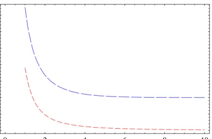
Note that νp is exponentially small. We have computed the radius of convergence Rp = 1/(µp+νp) of the inverse scattering series when Ω is a ball of radius 2a, whereais the radius of the ball containing the support of η and both balls are concentric. The dependence of
Rp on ka is shown in Figure 3. It can be seen that R∞ . 1 and R2 . O(1/(ka)3/2) when
ka≫1.
5. Scalar Waves
In this section we will analyze the inverse scattering series for the case of scalar waves. We will see that although the algebraic structure of the inverse Born series for diffuse waves is similar to that for propagating scalar waves, its analytic structure is different. This distinction underscores the underlying physical difference between the short-range propagation of diffuse waves and the long-range propagation of scalar waves.
Consider the time-independent wave equation
∇2u(x) +k2(1 +η(x))u(x) = 0 , x∈R3 (87) for the propagation of a scalar wave field u. The wave number k is a positive constant and
η(x) is assumed to be supported in a closed ballBaof radius a, with η(x)≥ −1. The fieldu is taken to obey the outgoing Sommerfeld radiation condition. The solution to (87) is given by the integral equation
u(x) = ui(x) +k2
Z
R3
0 2 4 6 8 10 ka 0 0.5 1 1.5 2 2.5 3 3.5 R
Figure 4. Radius of convergence of the inverse scattering series in theL∞norm for diffuse (— — —) and propagating waves (– – –).
where ui is the incident field and the Green’s function is given by
G(x, y) = e ik|x−y|
4π|x−y| . (89)
The convergence, stability and approximation error of the inverse scattering series corresponding to (87) is also governed by Theorems 3.1, 3.2 and 3.3. However, the values of the constantsµp andνp must be modified. The modifications are a reflection of the difference between the oscillatory nature of the Green’s function (89) and the exponentially decaying diffusion Green’s function. It can be seen that
µ∞ = 1 2(ka) 2 , (90) ν∞ ≤ k2|B a| (4πdist(∂Ω, Ba))2 . (91)
Thus the radius of convergence is R∞ =O(1/(ka)2) for ka≫1. This means that for small
scatterers, the inverse scattering series has a large radius of convergence, in contrast to the case of diffuse waves where R∞=O(1) even for large scatterers. The dependence of R∞ on
ka is illustrated in Figure 4 for both diffuse and propagating scalar waves.
6. Discussion
A few final remarks are necessary. Numerical evidence suggests that the estimates we have obtained on the convergence of the inverse series are conservative since kK1kp ≫ 1 in practice [10, 12]. Nevertheless, insight into the structure of the ISP has been obtained. In
particular, the inverse series is well suited to the study of waves which do not propagate over large scales such as diffuse waves in random media and evanescent electromagnetic waves in nanoscale systems [3, 2]. In the latter case, the inverse scattering series has also been shown to be computationally effective [15]. To analyze this problem, our methods must be extended to treat the Maxwell equations. Other areas of future interest include the study of the inverse Bremmer series [9].
Acknowledgements
We are very grateful to A. Hicks for making this collaboration possible and to C. Epstein for many useful suggestions. S. Moskow was supported by the NSF grant DMS-0749396. J. Schotland was supported by the NSF grant DMS-0554100 and by the AFOSR grant FA9550-07-1-0096.
[1] S. Arridge, “Optical tomography in medical imaging,” Inverse Probl.15, R41-R93 (1999).
[2] P.S. Carney, R. Frazin, S. Bozhevolnyi, V. Volkov, A. Boltasseva and J.C. Schotland, “A computational lens for the near-field,” Phys. Rev. Lett.92, 163903 (2004).
[3] P.S. Carney and J.C. Schotland, “Near-field tomography,” MSRI Publications in Mathematics47, 133-168 (2003).
[4] D. Colton and R. Kress, “Inverse Acoustic and Electromagnetic Scattering Theory,” Springer-Verlag, Berlin, 1998.
[5] A.J. Devaney and E. Wolf, “A new perturbation expansion for inverse scattering from three dimensional finite range potentials,” Phys. Lett. A89, 269-272 (1982).
[6] D. Gilbarg and N.S. Trudinger, “Elliptic Partial Differential Equations of Second Order,” Springer-Verlag, Berlin, 2001.
[7] R. Jost and W. Kohn, “Construction of a potential from a phase shift,” Phys. Rev.87, 977-992 (1952). [8] Y. Katznelson, ”An Introduction to Harmonic Analysis,” Dover, New York, 1976.
[9] A. Malcolm and M. deHoop, “A method for inverse scattering based on the generalized Bremmer coupling series,” Inverse Probl.21, 1137-1167 (2006).
[10] V. Markel, J. O’Sullivan and J.C. Schotland, “Inverse problem in optical diffusion tomography. IV nonlinear inversion formulas,” J. Opt. Soc. Am. A20, 903-912 (2003).
[11] V. Markel and J.C. Schotland, “On the convergence of the Born series in optical tomography with diffuse light,” Inverse Probl.23, 1445-1465 (2007).
[12] V.A. Markel and J.C. Schotland, “Symmetries, inversion formulas and image reconstruction in optical tomography,” Phys. Rev. E70, 056616 (2004).
[13] H.E. Moses, “Calculation of the scattering potential from reflection coefficients,” Phys. Rev.102, 550-567 (1956).
[14] R. G. Novikov and G.M. Henkin, “The ¯∂-equation in the multidimensional inverse scattering problem,”
Russ. Math. Surv.42, 109-180 (1987).
[15] G. Panasyuk, V. Markel, P.S. Carney and J.C. Schotland, “Nonlinear inverse scattering and three dimensional near-field optical imaging,” App. Phys. Lett.89, 221116 (2006).
[16] R.T. Prosser, “Formal solutions of the inverse scattering problem,” J. Math. Phys.10, 1819-1822 (1969). [17] J.R. Singer, F.A. Grunbaum, P. Kohn and J.P. Zubelli,“Image reconstruction of the interior of bodies
that diffuse radiation,” Science248, 990-993 (1990).
[18] G.A. Tsihrintzis and A.J. Devaney, “Higher-order (nonlinear) diffraction tomography: Reconstruction algorithms and computer simulation,”IEEE Transactions on Image Processing9, 1560-1572 (2000).
[19] M.C.W. van Rossum and T. M. Nieuwenhuizen, “Multiple scattering of classical waves: microscopy, mesoscopy and diffusion,” Rev. Mod. Phys.71, 313371 (1999).
[20] A. B. Weglein, F. V. Arajo, P. M. Carvalho, R. H. Stolt, K. H. Matson, R. T. Coates, D. Corrigan, D. J. Foster, S. A. Shaw, and H. Zhang, “Inverse scattering series and seismic exploration,” Inverse Probl.19, R27-R83 (2003).