An empirical macroeconomic model for policy design : the case of Chile

WORKING PAPERS

Macroeconomic Adjustment

M and Growth

Country Economics Department The World Bank

June 1991 WPS 709

An Empirical

Macroeconomic Model

for Policy Design

The Case of Chile

Luis Serven

and

Andres Solimano

A model focusing on the design and evaluation of

macroeco-nomic policy is applied to Chile.

ThePobly,Research, and l'xtemal Affairs Complex distnbutes PRIE WorkingPapers todisseminate the findungs of work inprogress and to encourage the exchange of ideas among Bank stalf and all others interested in development issues. These papers carry the names of the authors, renect only their views, and should be used and cited accordingiv. T'he findungs, interpretauons, and conclusions are the authors' own. They should not be atLnbuted to the World 13ank, its 13oard of Directors, its management, or any of its member counuies.

Public Disclosure Authorized

Public Disclosure Authorized

Public Disclosure Authorized

Macroeconomic Adjustmn and G:rowth

* J

WPS 709

This paper -a product of the Macroeconomic Adjustment and Growth Division, Country Economics

Department --- is part of a larger effort in PRE to design applicd macroeconomic models for the evaluation of mnacroeconomic policies. Copies are available free from the World Bank, 1818 H Street NW, Washington DC 20433. Please contact Susheela Jonnakuty, room N 1 1-039, extension 39074 ( 79 pagcs, with figu. i, graphs, and

tables).

Serven and Solimano construct, estimate, and consistent framework, the modcl adds behavioral simulate a macroeconomic model for Chile. equations with sound analytical foundations. This model allows aggregate supply and demand

factors to interact in determining such key Serven and Solimano use model simulations economic variables as inflation, the real wage, to explore the effects of domestic policies and the real exchange rate, real output and employ- external shocks (like a balanced-budget fiscal ment, and the current account balance. expansion, a policy of increased growth in

minimum wages, a fall in world copper prices, The model ensures the consistency of and an oil price shock). These simulations help different aggregates by imposing the relevanit illustrate the effects of economic policies and budget constraints on the fiscal sector, the ecntral external factors that shape current policy discus-bank, and the balance of payments. To this sions in Chile.

The PRE Working Paper Scries disseminates the findings of work under way in the Bank's Policy, Research, and Extemal AffairsComplex. An objective of the scxies is to get these findings out quickly, even if presentations are less than fully polished. The findings, interpretations, and conclusions in these papers do not necessarily represent official Bank policy.

1. Introduction ... .... ... .... .... . 1

2. The Chilean Economy in the 1980s: an Overview . . . 3

3. The Analvtical Model . . . 14

4. Empirical Results ... . 35

5. Out-of-Sample Policy Simulations ... . 48

6. Final Remarks . . . 61

REFERENCES . . . 62 TABLES

FIGURES

* We thank Bela Balassa, Vittorio Corbo, Stanley Fischer, John Holser,

Johannes Linn, seminar participants at ILADES. and our colleagues at CECMG for

useful comments on previous versions of this paper. Jorge Castillo, Raul

Laban, Fernando Quevedo and Rodrigo Vergara provided efficient research

The design and implementation of macroeconomic policies requires, among

other things, a clear understanding of the rules of macroeconomic behavior and

the budget constraints that relate macro variables. The development of

empirical macroeconomic models incorporating an adequate representation of

such relationships may be a useful tool for policy-makers and scholars

interested in macroeconomic policy. In the past fifteen years, empirical

macro modelling has suffered two lines of criticism: on the one hand,

traditional macroeconometric models have been criticized on the grounds that

their theoretical underpinnings are weak and because of their lack of solid

rmicrofoundations. A second line of criticism focuses on the fact that the

"structural" parameters of econometric models are in fact not policy-invariant

and therefore their use may lead to potentially misleading model-based policy

prescriptions and evaluation. This paper takes the view that in spite of the

validity of some of these ctiticisms, there is still room for

theoretically-grounded, empirically relevant, macroeconomic modelling.

Hacro modelling may be very useful in three respects. First, it

provides a conceptual framework organized around accounting identities and

behavioral relationships that can help in the uno'erstanding of macroeconomic

problems. Second, empirical macro models provide a quantitative tool for

assessing the orders of magnitude of the impact of different policies on the

main variables that are of interest in the conduct of macroeconomic policy.

And third, the models can help assess the consistency between targets of macro

policy such as low inflation, external balance and sustainable growth, the

setting of policy instruments for monetary, fiscal and exchange rate policy

and the level of certain key relative prices such as the real exchange rate,

the real interest rate and the real wage.

In this paper we set up a macroeconomic model for an open economy in

wnich both aggregate demand and aggregate supply play a role in the

determination of the key macroeconomic variables -- output, employment the

rate of inflation, the real exchange rate and the real interest rate. The

simulation of macro policies in the 1990s.

The analytical model considers the gooda market, the labor market, and

assets markets. Goods market clearing determines the real exchange rate. Among

the components of goods demand, private consumption anu investment as well as

exports and imports are endogenously determined. Aggregate demand depends on

current end permanent income, the real interest rate and fiscal parameters;

and on the real exchange rate and foreign demand. Aggregate supply of

domestic goods depends on real wages and also on the real exchange rate, due

to the use of imported intermediate inputs in the production process.

In turn, the 'Labor market need not clear in the short run, due to wage

inertia. The wage-exchange rate-price mechanism is also an important part of

the model. In particular, our framework intends te capture the impact of wage

indexation and exchange rate rules on the dy,.amics -- and, especially the

inertia -- of inflation.

Finally, the model ensures consistency by explicitly incorporating three

crucial constraints for the conduct of macroeconomic policy: the fiscal

constraint, the balance of payments, and the money supply identity.

The plan of the paper is as follows. Section 2 provides an overview of

the Chilean economy in the 19808 in order to set the stage for understanding

some macro policy choices envisaged for the 1990s. The analytical structure

of the model is presented in section 3. The results of the econometric

estimation are presented in section 4. In section 5 the model is used to :

perform a set of policy simulations for the period 1990-1995. A base

simulation is constructed in order to have a benchmark case to which compare

the policy simulations. The paper closes with some final remarks in

section 6.

2. The Chilean Economy in the 1980s: An Overview'

The behavior of the Chilean economy during the eightias can be

characterized by three clearly distinguished periods. The first one was

associated with an exchange rate based stabilization program following the

fixing of the exahange rate from mid-1979 to mid-1982. In that period

inflation sta-ilization was pursued through the management of exchange rate

policy, and an unsustainable debt-led boom in economic activity developed,

fueled by external borrowing. A second period comes in 1982-1983 where a

severe recession and a financial crisis set in associated with previous policy

mistakes and advertse external shocks. Finally, after 1984 emerges a period of

recovery and growth based in strong export performance and the recovery of

investment in a context of macroeconomic stability, impaired at the end of the

1980s by an unwarranted demand expansion.

2.1 Exchange rate based stabilization: 1979 82

This period is characterized b- a failed attempt at exchange rate-based

stabilization that begins ir- June 1979 when, after a moderate stepwise

devaluation, the exchange rate was fixed for an undetermined period of time in

order to curb inflationary expectations and bring domestic Inflation to

international levels. The absence of fiscal imbalances and a low (and

uniform) tariff structure were regarded as atrong backers of the exchange rate

policy. Ultimately, the experiment had to be abandoned in June 198g Len the

exchange rate was finally devalued in the midst of a severe recession and

worsened extern 1 conditions.

This period was one of booming economic activity, rising real wages and ;

overexpanding financial intermediation in a context of heavy foreign

borrowing. Severe misalignments in some key relative prices and foreign and

domestic overindebtedness rendered the economy particularly vulnerable to

adverse external and internal shocks. In fact the real exchange rate

appreciated and unsustainable current accounts deficits developed -- up to

14.52 of GDP in 1981 -- as exports started to be squeezed and imports boomed.

In turn, high domestic real interest rates, mainly in 1981, seeded an incoming

financial crisis as the path of internal debt accumulation by domestic firms

borroW.ng) reached unsustainable levels.

2.2 The crisie of 1982-83

During 1982-1983, the Chilean economy experienced a severo recession as

a consequence of negative external shocks and previous domestic policy

miGtak,s2. After an attempt to correct the large external imbalance developed

in 1981, through tight money and high real interest rates (without devaluing

the exchange rate), by mid-1982 the government changed its policy and decided

to correct the exchangie rate overvaluation by a series of 1iscrete

devaluations followed by a crawling peg. Fiscal and monetary policies were

clearly restrictive to support the exchange rate policy and reduce domestic

absorption. As a result of these policies and the external shocks, CDP fell

by around 1. percent in 1982-83, imports were cut by half in real terms in

those two years, investment collapsed and open unemployment rates climbed to

nearly 20 percent. The sharp drop in economic act vity during 1982-83 was

complicated by the financial situation of many indebted firms as they started

to face the coa4unction of large debts and depressed demand. As a result, the

financial sector was in a very fragile shape with an important part of the

loans of the major financial institutions becoming non-performing. The

banking crisis further curtailed the supply of domestic credit in the economy,

forcing ultimately the Central Bank to intervene several firnncial

institutions and undertake massive rescue operations and, in some cases,

liquidation.

2.3 The opriod of recovery and growth after 1984

A phase of recovery and growth takes place after 1984. In 1984-89 GDP

grew at an impressive 6.3 per year, and inflation averaged 20.4 percent per

annum, a low level for Latin American standards. In addition, such growth bqs

taken place in the context of reduced reliance on external savings (see the

2 There is an already vast literature on that period for the Chilean case,

Internal

financial

stability.

Looking at this porformance some important

questions

arises

First,

what ate

the

sources

of growth

in the

Chilean

economy

in this

period?

Is .he

current

growth

record

sustainable

over

time?

What

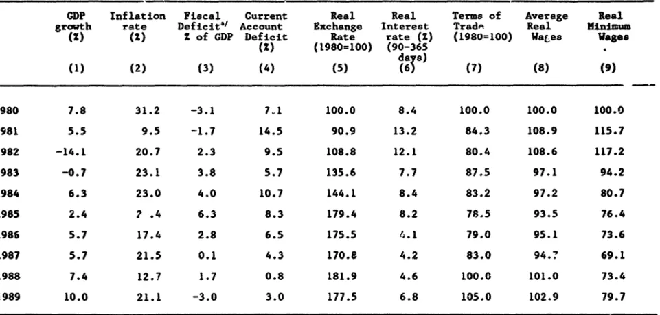
Table 1. Macroeconomic Indicators for Chile: 1980-89

GDP Inflation Fiscal Current Real Real Terms of Average Real

growth rate Deficit1 Account Exchange Interest TradA Real Minimum

(2) (2) Z of GDP Deficit Rate _{rate (Z) (1980=100) WaLes Wages}

(S) (1980=100) (90-365 da s8) (1) (2) (3) (4) (5) (6 (7) (8) (9) 1980 7.8 31.2 -3.1 7.1 100.0 8.4 100.0 100.0 100.0 1981 5.5 9.5 -1.7 14.5 90.9 13.2 84.3 108.9 115.7 1982 -14.1 20.7 2.3 9.5 108.8 12.1 80.4 108.6 117.2 1983 -0.7 23.1 3.8 5.7 135.6 7.7 87.5 97.1 94.2 1984 6.3 23.0 4.0 10.7 144.1 8.4 83.2 97.2 80.7 1985 2.4 7 .4 6.3 8.3 179.4 8.2 78.5 93.5 76.4 1986 5.7 17.4 2.8 6.5 175.5 4.1 79.0 95.1 73.6 1987 5.7 21.5 0.1 4.3 170.8 4.2 83.0 94.? 69.1 1988 7.4 12.7 1.7 0.8 181.9 4.6 100.0 101.0 73.4 1989 10.0 21.1 -3.0 3.0 177.5 6.8 105.0 102.9 79.7

Source: Boletin

Mensual

Banco Central de Chile. Various Issues.

CEPAL (1989) Informe Preliminar de la Economia de America Latina, el Caribe. Naciones Unidas.

explains the fact that thb recovery of economic

activity

in Chile has been

non-inflationatl.(by Latin American standards) in circumstances that the

exchange rate has depreciated over 45 percent. in real terms, in the last six

years and a financial crisis led monetary authorities to reshuffle major

financial intermediaries? To which extent the benefits from higher growth have

been shared by labor and other low income groups?

2.3.1 Sources of recovery and growth after 1984

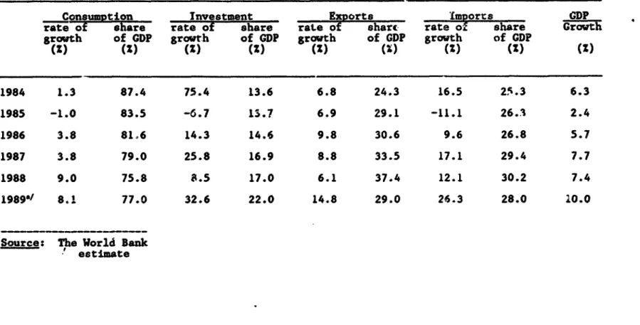
An important fact that table 2 shows is that the recovery in Chile since

1984 has been driven mostly by exports and investment, rather than by

consumption growth. In fact, the average rate of growth of total exports has

been 8.9 percent per year in the period 1984-89 whereas the rate of growth of

aggregate consumption has averaged 4.2 per year over the same period.

Investment has been growing at an average rate of 25 percent per year chough

with large fluctuations over the period; nevertheless, this percentage is

strongly affected by 1984 and 1989, when the growth in gross investment seems

to reflect, to a considerable extent, the building up of inventories. Anyway,

as a share of GDP, investment has recovered from a low of 13.6% in 1984 to 22

percent in 1989. Moreover, exports also have increased their share of GDP

while the share of total consumption hab declined.

What explairs the rapid increase in exports, investment and growth in

the last six years? exchange rate policy has played a preeminent role in the

expansion of exports and import competing activities in that period. A higher

Table 2. Sources of growth in Chile: 1984-89

Consumdtion Investment _Ex wrts inorts GDP

rate of share rate of share rate of share rate of share Groth

growth of GDP growth of GDP growth of GDP growth of GDP

(Z) (M) (S) (Z) (2)

(X)

(2) (X) (Z) 1984 1.3 87.4 75.4 13.6 6.8 24.3 16.5 25.3 6.3 1985 -1.0 83.5 -6.7 13.7 6.9 29.1 -11.1 26.3 2.4 1986 3.8 81.6 14.3 14.6 9.8 30.6 9.6 26.8 5.7 1987 3.8 79.0 25.8 16.9 8.8 33.5 17.1 29.4 7.7 1988 9.0 75.8 8.5 17.0 6.1 37.4 12.1 30.2 7.4 198Y' 8.1 77.0 32.6 22.0 14.8 29.0 26.3 28.0 10.0

Source: The World Bank

producing for external markets - a factor captured mainly by non-copper

exports. Thn increase in the basic tariff rate' from 10 percent to 20

percent (whose anti-export bias was more than offset by the real depreciation)

and indirest tax reimbuisement for export@ have also contr,.buted to the

expansion of the tradab,.a goods sector in general. In addition, the existence

of idle capacity (until 1987) and the ample availability of labor also

contributed to the expaniton of export and import competing activities.

Besides the positive impact of supportive macroeconomic policies and a

competitive real exchange rate on the very rapid expansion of non-traditional

exports in Chile (fresh fruit, fish, paper. timber) this process is also

related to institutional factors and structural change carried out in the

sixtics and seventies. The CORFO (Croporaci6n de Fomento de la Producci6i.,

plan of fruit growing (1968) and the afforestation activities of 1966-73 wera

two initiatives that boosted agricultural development and also the ability to

export in these arrRas. The agrarian reform of 1965-73 also contributed, in

spite of transitional problems, to help modernize the agricultural sector from

the latifundior (quasi-feudal) str cture. MoreovBr, after 1974 a new process

of land redistribution, sale b- tender and auctioning -- starting from the

structure left after the agrarian reform process -- took place. giving rise to

a more aczive land market that was needed to support a more oowpetitive

environment in agriculture.'

Total investment has been stimulated by various factors5. Besides the

recovery of public investment, the reduction in real interest rates

undoubtedly contributed to the recovery of private investment. A monetary

policy of real interest rate targets, conducted in the context of a financial

market characterized by the extensive use of indexed financial instruments.

' Specific import duties were imposed on some products where evJ.dence of

dumping was found.

' See ECLA (1990) for a further discussion of these issues for the case of

Chile.

s An econometric analysis _{of the behavior of private investment in Chile}

was the chief mechanism behind the interest rate policy.6 Tax incentives

seem to have played also an important role in the recovery of private

investment in Chile, as the tax rate on corporate incomes was reduced from 46

percent to 10 percent; in addition, reinvested profits received a preferential

tax treatment over dividends.

The average rate of growth of GDP in the Chilean economy was 8.7

percent during 1988-89 (10 percent in 1989). That ixceedingly high growth

record seems to reflect, to a considerable extent, two elements: the first is

related to an improvement in external conditions in the form of high copper

prices (a positive terms of trade shock) observed since 1987, and the second

is a political business-cycle feature, namely the adoption of a highly

expansionary monetary policy in the second half of 1988 -- Ml grew nearly 50

percent in that period -- as a plebiscite over the permanence of the military

regime was to take place in October of that year. In addition, given the

traditional lags in the effects of monetary policy on real economic activity,

the stlmulative effects of the late 1988 monetary expansion were largely felt

also in 1989. Moreover, the presidential and parliamentary election of

December 1969 was preceded by a rather lax monetary stance that rapidly

resulted in an acceleration of inflation in the last quarter of 1989.

Therefore an attempt to maintain a pace of growth thai. reflects, to a large

extent, cyclical elements, over a more extended period of time. would sooner

or later conflict with other targets of macroeconomic policy like muintaining

low inflation and the preservation of external balance. In that perspective,

since December 1989 the central bank is tightening monetary policy in order to

cool down growth. The actual deceleration in growth during 1990 has been

sharp and the forecasts for 1990 predict a rate of GDP growth of around 1-22

for the year (down from 102 in 1989).

6 According to Fontaine (1988). the level of the real interest rate was

determined on the basis of two criteria: to provide a reel return to domestic

financial assets competitive with the return of financial instruments abroad, so

to avoid capital flight and, second, the real interest rate should be consistent

2.3.2 Whv the adjustment of relative prices and the financial crisis was

non-inflationary in Chile?

An interesting issue mentioned before is the non-inflationary adjustment

of the Chilean economy, in spite of a large real depreciation of the exchange

rate -nearly 45 percent since 1984 (see table 1) -- and the turnaround of a

serious financial crisis that required massive Central Bank intervention.

Two explanations may be advanced in this regard.r First, the series of

devaluations starting in 1982 were accompanied by de-indexatio., of wages; thus

a real depreciation did not require a permanent acceleration in inflation in

order to reduce real wages. In addition, the increase in the rate of

unemployment, reaching levels over 20 percent in 1982-83 and remaining fairly

high until 1987, acted as a "labor market-deterrent" for workers attempting to

recover the level of real wages squeezed after the crisis of 1982. With ample

slack in the labor market. firms were not forced to bid up for additional

labor through higher wages (mainly for less skilled labor, where unemployment

concentrated) a factor that prevented an acceleration of inflation coming from

the wage side during the adjustment process. Clearly in Chile the "classical"

price-wage-exchange rate spiral resulting from an attempt to modify the reil

exchange rate while maintaining wage indexation and monetary accommodation

was absent. However the "Chilean way" was not costless in terms of economic

activity and real wages, though the costs were tilted towards the first phase

of the adjustment process.

A second factor refers to the fiscal situation. In Chile. like in

other highly indebted countries, the strain on the public sector accounts

resulting from the crises of 1982-83 centered mainly (but not only) on the

quasi-fiscal deficit (central bank budget). The deterioration stemmed both

from the increase in the domestic currency value of servicing the external

debt after 1982. and of the reecue program of troubled financial institutions

and conglomerates set-up by the Central Bank. These adverse quasi-fiscal

shocks have been non inflationary for two main reasons: first the

non-7 Sea Corbo and Solimano (1990) for an econometric analysis of inflation and

financial public sector in Chile ran a

surplus

In its primary deficit during

this period. transferring part of it to the central bank to cover its new

losses. Second, the rescue operations of troubled financial institutions were

carried out by issuing interest bearing liabilities of the central bank

rather than by issuing high powered money. The issuing of interest-bearing

liabilities by the Central lank was directed to finance debt-relief schemes

for borrowers of the banking system, to the purchase of risky loans by the

Central Bank with a (generous) repurchase obligation on the part oi banks'

shareholders and to the recapitalization and subsequent sale (financed with

government credit and subsidies) of intervened banks to small investors (the

"capitalismo popular" scheme)'. It is notevorthy to recognize that the whole

scheme of reshuffling the banking system involvod placing large amounts of

central bank bonds in the market. That required, of course, a corresponding

increase in demand for such assets. The rapid recovery of the Chilean economy

since 1984 in terms of growth of output, certainly was instrumental in that

regard (also because it helped increase private savings). In a medium-term

perspective, however, these new Central Bank interest-bearing liabilities

constitute a "latent inflationary pressure" that can be triggered if other

"non-monetary" sources of central bank revenues deteriorate in the future.

2.3.3 Incidence of the costs of adiustment and the benefits of recovery and growth

A key and difficult question is the social distribution of the costs and

benefits of the macroeconomic adjustment. Table 2 shows that average real

wages recovered their 1980s level just in 1988 and that minimum wages in real

terms were still 20 percentage points below their 1980 level and 35 points

under their 1982 level. That suggests that labor, and particularly low wage

groups, paid a significant share of the costs of adjustment in Chile. In

turn, the benefits for labor of the recovery after 1984 have taken more the

form of an employment increase rather than real wage growth. The step from

' See Larrain (1989) for a detailed account of the management of the Chilean

functional to personal income distribution is hard to make, particularly in

the case of Chile because of the absence of comprehensive information on

income distribution in this period. However, actions like the cut in some

items of social spending e.g., pension payments, and the squeeze on public

sector wages suggest that middle-low income groups also suffered in the

adjustment process. The incidence of the costs of adjustment on high income

groups is less clear since their income tax rates were reduced. Asset

transfers in the privatizations that took place after 1985 and the granting of

subsidies to the financial sector provide some clues that high-income groups

were shielded, in part, from the costs of adjustment.

3. The Analytical Model

In this section we set up a simple aggregate model for the Chilean

economy. We basically use an open economy IS-LM framework, extended to

incorporate the supply side and the labor market. We consider one single

domestic good' that can be used for consumption, investment, and exports, and

whose market must clear at every instant; goods market equilibrium determines

the real exchange rate and real output. In contrast. the labor market need not

clear in the short run due to wage rigidity.

The presentation of the model will start with the components of

aggregate demand and aggregate supply for domestic goods. Then we will turn

to the labor and assets markets, and provide a simplified representation of

the behavioral model. We close the discussion with the budget constraints of

the economic actors.

The Goods Market

Let us turn first to the demand side of the goods market. Aggregate

demand for domestic goods is the sum of public and private consumption and

' This may seem odd in view of the important role of copper in the Chilean

economy. The model assumes that copper is produced only for exports, and that the

production volume is exogenous. Sowever, copper revenues will be endogenously

investment. plus net exports.

The private consumption equation is based on the assumption that there

are two groups of consumers: the first group is liquidity constrained (they

cannot borrow in capital markets against their future income), so that their

consumption depends on current real disnosable income'0, Yd. The other

consumers (e.g. the wealthy, and upper-middle income groups) are

unconstrained, and determine their consumption according to the life

cycle-permanent income hypothesis (Hall, 1978); thus., their current consumption

depends on past consumption and on the unanticipated change to permanent

income, which can be summarized also by current disposable income. Aggregate

consumption Cp, is the sum of consumption of the constrained and unconstrained

consumers; hence it depends on both current income and lagged consumption:"

(1) Cp. -

Cp,(Yd,

CP.-J

Real disposable income is defined as:

(2) Yd - [pY - T - e*FFP]/pe

where Y is real output, p is the domestic price level, T are taxes, e is the

nominal exchange rate (units of domestic currency per unit of foreign

exchange), p, is the consumption ieflator, and FFP is net factor payments

abroad (in foreign zurrency terms). which are given by profit remittances PR

plus interest payments on net foreign debt:

(3) FFP - PR + i^-(FD-RE)

with PD and RE denoting foreign debt and foreign reserves, respectively.

10 For recent evidence that the role of liquidity constraints in consumption

is more important in countries with relatively less developed capital markets (as

most LDCs), see Jappelli and Pagano (1990).

11 We have omitted, just for simplicity, two possible extensions: first,

the distribution of income between wage earners and profit recipients could be

another determinant of consumption spending (Diaz-Alejandro, 1965). Second, the

ex-ante real interest rate could also affect private consumption -- although the

direction of this effect is theoretically (and empirically) ambiguous. In our

Private fixed investment is determined along the lines of the standard

cost-of-adjustment model (Hayashi. 1982). Thus, investment depends on Tobin's

Q, the ratio of the market value of installed capital to its replacement cost.

However, because of market imperfections, firms may find themselves rationed

in financial and/or goods marketsg hence, we must also allow for a direct

effect of current profits and demand conditions'2 _{on investment. Demaad}

conditions are measured by the degree of capacity utilization in the economy

Y/Yp, where Yp denotes potential or full-capacity output. In turn, with

variable production inputs (labor and materials) optimally adjusted, current

profits can be shown to depend only on the degree of capacity utilization. In

summary, private investment can be expresSedQd

(4)

Ipr - Ip, (Q. Y/Yp)

In turn, Tobin's Q depends on anticipated profits and the real interest

rate", r. As before, profits are summarized by the degree of capacity

utilization, Y/Yp:

(5) Q = q(r, Y/Yp)

Government consumption, C₆, and public investment, I., are considered

policy determined variables so they are exogenously given.

Real copper exports X.w are exogenous; in turn, non-copper exports X;

are endogenously determined. They depend on the price of competing foreign

goods relative to the price of the domestic good ep*/p, and on the level of

12 For a formal proof that when the firm faces sales constraints the optimal

investment rule depends on both Tobin's Q and goods demand, see Precious (1985).

"3 For notational simplicity, all behavioral equations are written as

static. However, in their empirical implementation we will allow for dynamic

effects.

" More precisely, Tobin's Q can be shown to equal the present value of

future unit profits, discounted at the real rate of interest plus the

depreciation rate of capital, (r+5). Under static expectations, this equals

current profits divided by r+S. In turn, with profits described by the degree of

world

demand

Y:

(6)

X.

X

(Sp,/P.

Y')

Real imports depend on the tariff-inclusive relative price of

importables in terms of domestic goods, ep (l+t)/p. where p' is the world

price of importable., and on the level of output Y:

(7) M - m(ep.(l+t)/p. Y)

Equating output to aggregate demand, we have:

(8) Y m Cpr + C6 + Ipr + Is +

Astk

+ X¢o + X - M

where Astk denotes inventory investment, which is exogenously determined.

On the supply side, we assume that output is produced according to a

constant returns to scale technology that uses labor, capital and imported

materials. Assuming profit maximization, we can write the supply function as

(9) Y/Yp - ye(w/p, ep*./p. p)

where w is the nominal wage rate, p'₃ is the foreign-currency price of

imported materials", and p is a productivity parameter. Solving for p. we

can write the inverse supply function as

(9') p - p(w. ep"*, p. Y/Yp)

which expresses the price of domestic goods p as a (variable) markup over unit

variable costs, with the markup rate increasing with the degree of capacity

utilization Y/Yp". Moreover, equation (9') must be homogeneous of degree one

in input prices.

Finally, the change in the level of capacity output is related to the

I Here we are assuming, only for notational simplicity, that the world

price of foreign materials in terms other importables is constant.

14 Notice that in principle this markup specification would be consistent

path of the capital stock:

(10) &Yp/Yp - AK/K

and the capital stock changes over time according to net investment:'7

(11) AK - (Ip,+Is) - 6K

The Labor Market

Because of wage stickiness, the labor market need not clear in the short

run. Labor supply equals the labor force L; actual employment is always

determined by labor demand. The specification of the latter follows from

profit maximization; hence, labor demand is related to the real wage w/p and

the level of output Y:

(12) L - 1( w/p. Y)

The rate of unemployment is defined as

(13) u =

1

- L/L

The labor market is completed with an equation describing the rate of

change of the average nominal wage w. The latter depends on four factors.

First, the rate of change of the consumer price index Apj/p0, reflecting

inflationary expectations and/or the existence of wage indexation. Second, the

rate of change of the minimum wage Awmin/vmin, which affects the average wage

directly through a "composition effect" (since a fraction of the workers earns

the minimum wage) and also through an indirect "relative wage" effect, which

links the whole structure of wages to the minimum wage. Third, the degree of

slack or excess supply in the labor market measured by the rate of

unemployment u, along the lines of a Phillips curve specification. Finally,

wage growth depends also on labor productivity g,,. Formally.

17 Here we are making the simplifying assumption that public and private

(14) Aw/w - v(Ap./p, Awmin/wmin, u,

)

The Money Market

We use a very simplified representation of assets markets. There are

three assets in the economy: money, domestic interest-bearing assets o, and a

foreign bond; the latter two assets are imperfect substitutes. Moreover, we

assume that there are barriers to capital mobility; hence, the private sector

cannot adjust instantaneously its holdings of foreign assets"'. In addition,

we assume that the nominal exchange rate is fixed (or managed by the

authorities).

We can su-arize portfolio equilibrium by considering the money market.

Formally, real money demand h depends on the nominal interest rate i, the

level of output Y, and the foreipn interest rate, i-. adjusted by the expected

rate of devaluation of the exchange rate, Alne. Hence money demand is

(15) h - h(i, Y, is +

Alne')

Letting H denote the nominal money stock, money market equilibrium implies

(16)

H/P = h(i, Y, iC +

Alne)

or, solving for the domestic nominal interest rate,

(16') i i( H/p, Y, i + Alne')

In turn, the domestic real interest rate r is equal to the difference

between the nominal interest rate i and the anticipated inflation rate We:

17)

r

- i - w

IS The domestic asset implicitly includes public debt and the claims on the

capital stock -- i.e., holdings of equity. This amounts to assuming that domestic

debt and equity are perfect substitutes (up to a constant risk premium).

19 This assumption ensures that at every instant the money stock is predetermined; however, we could eliminate it without any analytical

complication.

Also,

we could

allow

explicitly

for a parallel

foreign

exchange

market

without

major

difficulties

(other

than

empirical).

Price Defipitions

The model is completed with two equations describing the consumption and

investment deflators. Both consumption and investment are assumed a composite

of domestic goods and imports. Hence their implicit deflators can be expressed

(18) P a Pc(P. eep' (1+t))

(19) Pk P

Pk(P'

e9p*.(1+t))

where Pk iS the investment deflatorl further, both p, and pk must be

homogeneous of degree one in p and eop (l+t).

Finally, the national accounts nominal income-expenditure identity can

be written

(20) pY - p,e(Cpr+Cg) + pK*(Ip,+It) + p,st,Astk + e*(p*4OeXCOP+p*X.-p%M)

where p*₀op is the world price of copper, which is exogenously given; equation

(20) is used to determine the deflator of inventory investment P.tk*

A SimRle GraDhical Regresentation of the Model

We can provide a simple graphical representation of the model by

reducing it to three equations depicting aggregate supply, aggregate demand,

and the current account balance, all in terms of the real exchange rate, real

output, and for given values of the remaining variables. First, a semi- p ;

reduced form for aggregate demand AD can be obtained by replacing equations

(1) through (7), (16'), and (17) through (19), into (8):

(21) AD - AD(ep-/p, H/ep-, a4)

where ad * (Cs, IB, TD, t, (FD-RE]/p*, PR/p', Y, i*, Alne*, p*/p**, X0op, P*Op/p*,

ir, Cp-1), and in arriving at (21) we have used the fact that H/p

(H/ (ep*)) (ep*/p).

given real money stock in terms of foreign goods H/(ep*)20, the AD schedule is

depicted in Figure 1 as an upward sloping l ne in the real exchange rate-real

output space (et. Y), reflecting the assumption that a real depreciation of

the exchange rate raises aggregate demand -- that is, the positive effect of a

real depreciation on net exports dominates its negative effect on real

disposable income and consumption. which is due to the increase in the value

in terms of domestic goods of foreign debt servicing payments, and in the

decrease in the value in terms of consumption goods of a given disposable

income in terms of domestic goods21.

The position of the AD schedule is determined by the values of the real

money stock H/(ep') and the other variables included in ad (i.e., all the

variables other than e₃ that affect aggregate demand) 22

In turn, the aggregate supply schedule AS is just given by (9).

rewritten here as

(22) AS = AS(ep*/p, w/(ep-), a.)

where a, a {(, Yp, p'₃/p'), and we have used the fact that w/p

(ep'/p)(w/(ep')). Thus, for givo.r a. and given real wage in terms of foreign

goods, the aggregate supply schedule is downward sloping in Figure 1,

reflecting the fact that a real depreciation increases the relative price of

imported materials (as well as the product wage w/p for given w/(ep*)) c.ad

20 Here we are making the important assumption that anticipated inflation

and depreciation are predetermined.

21 In Solimano (1986) a macro model of a devaluation is set up and

parameterized with Chilean data. The main result ie that a real depreciation

turns out to be contractionary in the short run followed by an expansion in

output and employment in the medium to long run. A real depreciation may affect

adversely absorption also via a cut in investment due to higher cost of imported

capital or because of a reduced access to credit by firms overindebted in

dollars. See Serven and Solimano (1990' for a full review of the effects of a

real depreciation on investment.

22 Note also that the inclusion of lagged consumption in ad gives rise to

a distinction between short run and long run equilibrium. The short run AD

schedule will be shifting over time as the economy approaches a stationary

equilibrium. In our empirical model this is more so, as other lagged endogenous

variables (e.g., exports or the real exchange rate) would also be included among

thus reduces output supply. A step beyond would be to insert the laws of

motion of the nominal wage and the capital stock (equations (11) through (14))

in (22). bringing out the dynamics of aggregate supply -- and allowing for a

distinction between the short run and long run aggregate supply schedules.

Finally, the current account deficit measured in terms of domestic goods

CA is given by

(23) CA - (e/p)

i*

(FD-RE) + PR -

FTR

+ p.OM - p.p&-

pPX,¢]

where FTR are net foreign

transfers;

the term (e/p)@(p M - p4 0 00cXp - p*XJR is the resource deficit. Inserting equations (6) and (7) in (23) we get:

(24) CA = CA(Y, ep'/p, iL,

(FD-RE]/p*,

FTR/p-. X,., YV. P-*/P*. P*-/P*)

=

CA(Y,

ep*/p.

a..)

Setting the right-hand side of (24) equal to zero, we obtain the CA

locus in Figure 1. which represents the combinations of output and the real

exchange rate that yield a balanced current account for given values of all

the other variables. The locus slopes upward, due to the fact that an

expansion in output raises imports and hence the resource deficit, and must be

compensated with a real depreciation in order to maintain the current account

in equilibrium. Points above the CA locus correspond to current account

surplus; points below correspond to current account deficit.

The domestic goods market clears when aggregate supply and demand are

equal; in Figure 1, this happens at point E. In the figure we have assumed

that E also corresponds to a balanced current account; hence, at E the economy

is in full macro equilibrium: the levels of the real exchange rate and output

are consistent with both internal balance2" (aggregate demand = aggregate

supply) and external balance (equilibrium in the current account).

Of course, the meaning of "internal and external balance" in our

2 A related issue is that of the stability of internal equilibrium. A

sufficient condition for static stability is that the aggregate demand schedule

be upward sloping, as assumed here. The dynamic stability under rational

expectations of a model similar (but somewhat simpler) to ours is examined in

framework must be qualified: on the one hand, internal balance may occur with

unemployment in the short run. On the other hand, external balance may be

consistent with a sustainable deficit in the current account, and not

necessarily with a zero deficit.

Tne functioning of the model can be seen by performing a simple

comparative static exercise, such as an increase in public spending that

shifts down and to the right the aggregate demand schedule in Fig,-re l(a)

(dotted line). The new short term equilibri m would be at E' where the real

exchange rate appreciates and the level of output increases (assuming output

is below full capacity). At E', however, there is now a deficit in the

current account which has to be financed either through an increase in

external borrowing and/or running down international reserves.

Another exercise of interest is a devaluation (i.e., an increase in e).

Of course, if a nominal devaluation is to have an impact on real variables, it

must not be accommodated by proportionate increases in nominal wages and the

nominal money stock; otherwise, as is clear from (21) and (22), real variables

would be completely unaffected, while p. v and H would all rise in the same

proportion as the nominal exchange rate.

In Figure l(b), we depict the effects of a devaluation holding constant

the nominal money stock and the nominal wage. From (21) and (22) it is clear

that both the real money stock and the real wage in terms of foreign goods

must fall, and thus the AS and AD schedules shift upwards; the CA schedule is

unaffected. Hence the outcome is a real depreciation and a current account

surplus; however, the effect on real output is in principle uncertain,

although if the adverse impact on interest rates and hence on investment

demand is not too large, output should be expected to rise, as represented in

E' in the figure.

Let us consider the determination of the rate of inflation by looking at

the dynamics of aggregate demand and aggregate supply. This is useful for

addressing ptoblems of inflation stabilization and to examine the inflationary

particular the issue of inflati.L inertia.

We can .1lvstrate these iss:iis as follows. First, equating aggregate

demand with aggregate supply.

AD( ep*/p, H/(ep*) 9 ad) - AS( ep'/p. w/(ep*), a,)

and solving for the rate of change of the price level n, we have

(25) -- a (Aw/w) + b (Ae/e) + c (QH/H) + v

where a+b+c.1, v is a function of the rates of change of a, and ad, and

foreign prices have been assumed constant. For given v, the rate of inflation

is a weighted average of the rate of wage inflation, the rate of devaluation

and the rate of cnange in the money supply; in turn, inflation may rise or

fall due to the effects of supply and demand shocks (the v term).

We can use (25) to illustrate the effects of the wage formation process

and exchange rate rules on inflation. Assuming a linear functional form for

the rate of change in nominal wages we can write equation (14) as:

(26)

Aw/w

- (1-9)OWC + Bs(Awmin/wmin) -

7*u

0

c a c l

where ¢r is the rate of change of the consumption deflator; y>OS and for simplicity we have ignored productivity growth. Hence the rate of change in average nominal wages is a function of consumer inflation. the rate of change in minimum wages, and the rate of unemployment. Let us assume that the minimum wage is indexed to current and past inflations

(27) Awmin/wmin - (1-9)rw + Ow,,_1 + k 0 < a 1

where k is an exogenous minimum wage shock. Replacing (27) in (26). we can write

(26')

Aw/w

- Sk= 3k-

59(ir

₀ -

7c..y)

u

which implies that, given k, the real consumption wage can only be reduced by

accelerating inflation (as long as 8>O) or through unemployment. On the other

of domestic goods in the consumption basket. Finally. let us assume that money

growth and nominal depreciation partially accomiodate inflation; hence Ae/e

-,. and AH/H ft where

O04,0cI.

With all these ingredients, we can rewrite

(25)

as

(28)

w

'

-

-

'u + vI

where a * D-'a890A+(1-A)9], 7'U D-'7, v'u D-l(v+k), and D a

1-bq-c'y-a(l-89)(A+(1-A),X]>0. Equation (28) shows that inflation depends on three factors:

lagged inflation, unemployment, and exogenous supply, demand, and minimum wage

shocks. In particular, the degree of inflation inertia is measured by a.

Hence, as can be directly verified, the larger the weight of minimum wages in

average wages E. the larger their backward indexation 9, and the more

accommodating money and exchange rates are (i.e.. the larger 0 and q). the

more persistent inflation is. In particular, with full accommodation (.-4=1),

(28) reduces to

(28')

-- w -

(a&90)Y^u

+ (aBO)-'(v+Bk)

so that current inflation fully reflects past inflation, irrespective of the

degree of backward indexation 9; however, the larger 0, the more costly in

terms of unemployment it is to reduce inflation below its past level.

Budget Constraings

The behavioral model is completed with the budgetary identities of the

different economic actors - that is. the private, public, and external

sector. These ensure the consistency between stocks and flows in the model.

which is necessary for the simulations to be of any practical interest.

One important issue is the appropriate degree of disaggregation of the

public sector. Normally, for the purposes of macroeconomic analysis, it would

suffice to consider the consolidated financial and nonfinancial public sector

-- that is, including the Central Bank. However, in the Chilean case the

problems, due to the large stock of Central Bank debt to the private sector,

and to an equally large stock of foreign-currency denominated liabilities of

the Government with the Central Bank. In order to keep close track of the

fiscal implications of these two issues, we choose to consider these two

agents separately.

To adapt the budget identities to the Chilean institutional context, we

must take into account two facts. First, most domestic currency financial

instruments (with the obvious exception of the money stock) are indexed to the

price level. The interest actually paid on such instruments is given by a

market determined 'real' interest rate applied to the actualized (i.e.,

according to inflation) principal of the instrument.

Second, the way in which the nonfinancial public sector (more precisely,

the central government) services its main liability with the Central Bank

(which has the form of a dollar-denominated Treasury note held by the latter)

is somewhat special. The liability originates from the consolidation of past

transfers to cover the Central Bank's operating losses. Interest on the

Treasury note accrues at a rate equal to LIBOR plus a fixed spread. However,

the actual interest payment by the government is only 2 percent of the

principal; the remaining interest accrued is capitalized. Moreover, the

government can also make anticipated amortization payments to reduce the

principal of the note".

Keeping these issues in mind, we can now describe the budget constraints

of the model. First, the identity of the external sector is just the Balance

of Payments, which in terms of foreign currency can be written

(29) P

*°M

- (P*07, +

P',peX,Op)

- FTR + (PR + i**(FD-REj) - DPI +

A[FD-RE]

Here DFI is direct foreign investment; all variables (with the exception

of real imports M and real copper and non-copper exports XCOp and X.,) are

measured in foreign currency (dollar) terms. The left-hand side of the

24

For example, in

1990 the government made an amortization payment of US

equation is the current account deficit described before; the right-hand side

is the capital account balance. Again, the term in square brackets FD-RE

represents pet foreign debt.

In turn, the budget constraint (in nominal terms) of the nonfinancial

public sector can be written

(30) (p,*Cg + GTR1b +

OE

+ ropO[b. + dc,]+ eoiO1FD, - CSF?)

- (TD + TI + OR + CUR) + pk*I₈

n p@(Adc, + abs) + e*AFDg -

eo(TBAmort

+ ACSF)

The first two lines of (30) represent the public deficit. The first term in

brackets represents current expenditures; the second, current revenues. Here

TD and TI respectively denote direct and indirect tax revenue in nominal

terms; CUR represents nominal revenue from copper production (i.e., the

pre-tax operating surplus of the public copper company); OR and OE are other

current revenues and expenditures2", expressed in nominal terms; CSF is the

'Copper Stabilization Fund', which we describe below; and GTR0b is a transfer

to the Central Bank. also expressed in nominal terms, which corresponds to the

interest paid on the Treasury note held by the Bank. Letting TB denote the

principal of the note (in dollars), GTRCb is determined according to

(31)

GTRCb - oOe*TB

where a is a given parameter (currently equal to 2 percent, aS explained

above). In turn, copper revenues are related to copper prices and exchange

rates by the following equation:

(32) CUR = (eSP*,, - 9P)OYS"

where

a

is a cost parameter, and Yd,. denotes the volume of public copper

production. Thus, nominal production costs are assumed to rise one for one

25 OR includes basically nontax revenues of the government and the operating

*urplus of public enterprises other than the copper company. In turn, OG mainly

with domestic prices.3'

The bottom.line of the public sector's budget constraint reflects the

change in the net liabilities of the nonfinancial public sector. Here dc, and

ba are the net domestic credit from the Central Bank2" and net public debt

held by the private sector, respectively, and they are defined in real terms;

hence, the corresponding interest payment is determined by the real interest

rate times the adiusted value of the principal, where the latter is determined

by the price level. In turn, PD. is net foreign debt of the nonfinancial

public sector.

The last two items in the right-hand side of (30) are somewhat unusual

and deserve separate comment. First, TBAmort represents the amortization

payment made by the government on the foreign currency-denominated Treasury

note held by the Central Bank2 ; its amount is arbitrarily determined by the

government. The principal TB evolves over time according to

(33) ATB I=*TB - (GTRcb/e) - TBAmort

so that if no amortization is paid, then the change in the principal plus the

current transfer received by the Central Bank add up exactly to i'*TB, i.e.,

the (spread-inclusive) world interest rate2" times the principal of the

Treasury note.

In turn, CSF is the 'Copper Stabilization Fund', expressed in

dollars'°. It represents a government account at the Central Bank to which a

fraction of copper revenues is deposited whenever the copper price exceeds a

26 Actually, part of the operating costs of CODELCO correspond to cop er

purchases and thus are related to copper prices. For simplicity, we ignore this

in (32).

2' According to the new regulations in Chile, the Central Bank is forbidden

from lending to finance public deficits. Hence, Ado, cannot be positive.

26 Notice that such note is not included in dc.

29 As described above, i would equal LIBOR plus a fixed spread.

3O

Again, the copper fund is not included in net credit from the Central

specified upper bound, and from which withdrawals can be made when the price

falls below a likewise specified lower bound. In summary. we can write:

(34) ACSF - p y

-here 0<1 (and not necessarily positive), and its precise value depends on the

world price of copper relative to the specified upper and lower bounds31.

Finally, we have the Central Bank's budget identity:

(35) e9i^6(FD.b-RE) - rep*(dc 5 + dcp,) - GTRCb + eoi*CSF

-ISB

+ e*A(FD¢b-RE) - pA(dc₈

+dcpj)

+ e*(TBAmort+ACSF)

The top line of the equation is the operating loss of the Central Bank,

with dcpr denoting real net credit to the private sector32; thus, the loss

equals the interest paid on net foreign liabilities minus the interest

received on net domestic assets (excluding the Treasury note), minus the

transfer from the government, plus the interest paid to the latter on the

Copper Fund.

The bottom line again denotes the change in the net liabilities of the

Central Bank which finances its net operating loss. It comprises the increase

in the money base HB, and in net foreign indebtedness, the decline in net

domestic assets, and the payments received from the governmeut for deposit to

the Copper Fund and for amortization of the Treasury note3

In the model, the monetary base is related to the money stock H by the

money multiplier p, which is assumed exogenous:

(36) H * IASHB

" Alternatively, we could have defined de, as net of the copper fund CSF and

of the Treasury note TB. The approach used in the text intends to highlight the

important role of these two items in the Central Bank-Central Government link.

1 Net, in particular, of domestic debt of the Central Bank held by the

private sector. hus, in the Chilean case dep, is negative.

33 Obviously, if the operating lose is zero and if there are no government

payments to the Copper Fund or for amortization of the Treasury note, the

To conclude the presentation of the budget identities"'. it may be

instructive to consider briefly the budget constraint of the consolidated

public sector, including the Central Bank. Suminig (30), and (35), this can be

written

(36) p¢*C. + OE + r*polb, - dc,lJ + eei**[FDS + PDb - RE]

-

(TD

+

TI

+

OR

+

CUR)

+

pkeI

8

m

poMbs

- dcp,l +

e@A(FD,

+ FDb - RE) + AHB

where (FD,+FDCb-RE) and p*(b.-dcp,) respectively are the net foreign and

domestic debt of the overall public sector. Using the money market equilibrium

condition (16) along with (33). and after some well known manipulations, we

can rewrite (36) in compact form as

(36')

def

+ rob + tr* + (Ae,/el)]f =

Ab

+ bf + (1/p)*(Ah(.) +

*h()]

where

def

a (poC$ +

OE

-

(TD

+

TI

+

OR

+

CUR)

+ pk-l,

I/p

is the

primary

deficit of the overall public sector in real termas b a b.7dcpr is the real

domestic debt stock; f E (e/p)*(FDi+FD.b-RE) is the real value of the net

external debt stock of the public sector in terms of domestic goods; r a i*-f*

is the foreign real interest rate; et denotes the real exchange rate, as

before; and h(.) is the money demand function (15).

The left-hand side of (36') is the inflation-adjusted deficit of the

overall public sector, which includes the real primary deficit plus real

interest payments on domestic and foreign debt; observe that the real interest

rate relevant for foreign debt is the world real iinterest rate plus the rate

of depreciation of the real exchange rate' Aede₁

.

The adjusted deficit must

" In principle, the model would also include a budget constraint for the

private sector. However, such equation can be shown to be a linear combination

of the budget constraints of the other sectors and the National Accounts

income-expenditure identity (20), and thus it need not be considered explicitly.

35 Obviously,

with

unrestricted access to foreign and domestic financial

markets, the optimal financial strategy of the public sector would be to

diversify its sourc i of financing only if r -

r'.&ee

1S. This has been emphasized

be financed by increasing the real stocks of foreign and/or domestic debt, or

by seigniorage revenues (the last term on the right-hand side).

In order to ensure that public debt will not eventually grow without

bound, we must require that real interest payments on the debt stock be met by

future primary surpluses and seigniorage revenues (where the latter include

the increase in real balances plus the inflation tax revenue)3 6. In terms of

the model, this can be done by imposing simple fiscal (or quasi-fiscal) policy

rules, such as assuming that increases in debt service are matched in every

Period by tax increases (as in, e.g., McKibbin and Sachs (1990)). While this

can be easily done, it would unnecessarily limit the ability of the model to

explore some quite realistic scenarios of 'sustained' fiscal imbalance. A more

flexible approach is to allow for arbitrary fiscal imbalances in the short to

medium term, while imposing fiscal adjustment in the longer term.

4. Empirical Results

4.1 Preliminary Issues

The structural model summarized in the previous section consists of

eleven estimable equations: four for the components of aggregate demand

(private consumption, private investment, imports, and non-copper exports),

three goods prices relationships (the inverse supply schedule, and the

consumption and investment deflators), two labor market equations (for

employment and nominal wages), and two asset markets relationships (for

Tobin's q and the domestic interest rate).

36 Formally, integrating (35") under the assumption that debt does not

explode in the ong run, we can write the intertemporai budget constraint of the

public sector as

b(t) + f(t)

Go

f

exp{-R(s))@((^h(s)+ir(s)*h(s))/~ - def(s)] ds +

f

exp(R(s)-R*(s)}*f(s) ds

t t

s 5

where R(s) a

I

r(v) dv, R (s) a I (r(v)+Ase(v)/et(v)] dv. That is, the existing

t t

debt stock must equal the present discounted value of future primary surpluses

plus ssigniorage revenues, plus an additional term that adjusts for the

discrepancy between domestic and foreign (real depreciation-adjusted) real

As written above, the behavioral equations (with the only exception of

that for private.consumption) contain no dynamics. However, in reality we must

allow for the slow adjustment of the left-hand side variables to their

'target' levels. For example, decision and delivery lags in the case of

investment, or slow market penetration in the case of exports, can account for

substantial differences between the short- and long-run responses of

investment or exports to their determinants. Thus, in our empirical equations

we included lags of the dependent and/or independent variables to capture this

lagged adjustment effects. In most cases, a standard cost-of-adjustment model

proved sufficient.

In principle, efficient estimates of the model's parameters could be

obtained from a joint estimation technique (e.g., three-stage least squares or

full information maximum likelihood). However, the available sample (which

includes fewer than 30 data points) is 'undersized', as the sample size falls

short of the total number of predetermined variables in the model. In such

context, the maximum likelihood estimator is not well defined (Sargan (1975)),

nor is the 3SLS estimator (as the instrument matrix fails to have full column

rank). Alternative system estimators based on instrumental variables have

been proposed in the literature (see e.g., Swamy (1980)); each one of them

results from a particular set of restrictions on the set of instruments

employed in the estimation, and therefore can be interpreted as imposing

implicit (and arbitrary) restrictions on the model's reduced form parameters

(for a discussion, again see Swamy (1980)). However, the relative advantages

of the alternative estimators are not entirely clear, as the comparisons of

performance often rely on asymptotic arguments which by definition are of

little interest in the context of small samples. Finally, the computation of

some of the system estimators for undersized samples can be rather cumbersome

(e.g., Brundy and Jorgenson (1971)).

On the other hand, joint estimation techniques pose the well-known

problem that misspecification of any equation will 'contaminate' the rest of

In view of these facts, we decided to estimate the model using 2SLS

equation by equation, with different sets of instruments for each equation".

In this manner, we avoid the problem of contamination - at the cost of some

possible losses in efficiency, which in an undersized sample such as ours are

not likely to be of great significance.

4.2 Estimation Results

The equations of the model were empirically estimated using annual data

for the years 1960-1987. Overall, the estimated equations provide reasonably

good fits; none shows any symptoms of serial correlation. All the parameter

estimates carry the theoretically correct signs. In most equations we tested

some specific parameter restrictions and, when not rejected, imposed them.

Such constraints raise the precision of the estimates and also contribute to

make the simulation results more easily interpretable. In some cases, the

constraints are dictated by basic economic theory (e.g., behavioral rules for

real variables should be homogeneous of degree zero in all nominal

magnitudes), and their rejection would be a symptom of misspecification. In

other cases, they make the dynamics of the model more reasonable (for example,

when imposing a unit long-run elasticity of consumption with respect to

disposable income).

Below we describe briefly each one of the empirical equations.

Goods Market

Private Consumption - As stated in (1), the estimated equation relates

real private consumption to real disposable income and to lagged consumption;

attempts to find a significant role for the real interest rate, credit

availability, or income distribution, proved unsuccessful.

The selected equation is:

" A possible extension of this procedure would be 3SLS with different

instruments for each equation (Schmidt (1990)). Of course, this would again lead

to inconsistent estimates in all equations if any one of the model's equations

(37) Log(Cpr) - - 0.069 + 0.578 Log(Cpr(-l)) (-2.863) (5.757) + 0.422 Log(Yd) - 0.194 D74 (5.757) (-5.742) R2 - 0.964 DW - 2.105 h - - 0.320 Adj-Ra a 0.961 F = 321.545 Sample: 1961-87

2SLS. instruments a Log(Cpr(-l)). Log(Yd(-1)). Trend, D74.

The adopted specification incorporates the constraint of a unit log-run

elasticity of consumption with respect to disposable income; the constraint

was not rejected by the data.

The consumption deflator - The implicit price of consumption was assumed in

(18) a weighted average of the prices of domestic goods and imports (with the

latter adjusted for tariffs). We used a first-difference specification:

(38) ALogPc 0.893 ALogP X 0.107 ALogle*P-,(1+t)) + 0.060 d74

(26.920) (26.920) (2.261)

R2 - 0.9980 DW - 2.271

Adj-R2 - 0.9979 F - 12004.61

Sample: 1962-87

2SLS; instruments - ALogP(-1). ALog[e9P",(1+t)J(-1). Log(P%Op), d74

The weights of domestic and import prices are constrained to sum to

unity, and the regression constant is restricted to zero; neither constraint

was rejected by the data'.

Private fixed investment - As described in (4), private fixed investment is

related to Tobin's Q (defined as the stock market index relative to the

investment deflator) and the level of output relative to full capacity".

The estimated equation is of the lagged adjustment form, and is written in

" Observe that a zero constant term amounts to ruling out a long-term trend

in the relative price of consumption.

terms of the (real) share of private investment in GDP:

(39) Log(lpr/Y) - 1.437 + 0.124 Log(Q) + 0.795 Log(Y/YP)

(-4.556) (2.996) (2.008) + 0.372 Log(Ipr(-1)/Y) - 0.472 D72 (2.849) (-3.027) Ra 0.7493 DW - 1.723 h - 0.947 Adj-R2 - 0.7016 F - 15.693 Sample: 1962-87

2SLS; instruments c Log(Q(-1)). Lo ( Y(-1)M

A?-1)

),

Lo (Ipr(-1)).

LogPc~, r-2), Trend i (-I) Lo4*-1)), D72

Thus, in the long run the investment share rises more than one for one

with the degree of capacity utilization. In turn, the long-run elasticity of

investment with respect to Tobin's Q is about .2. somewhat smaller than that

obtained by Solimano (1989) from the estimation of a similar equation with

quarterly data.

The investment deflator - As in the case of consumption. the investment

deflator in (19) is a weighted average of the GDP deflator and the import

deflator. A first-difference specification proved adequate:

(40) ALogPk = 0.856 ALogP + 0.144 ALogleP*K(1+t)] + 0.099 d7172

(16.506) (16.506) (3.505)

R2 = 0.9948 DW - 2.059

Adj-R' - 0.9946 F - 4581.25

Sample: 1962-87

2SLS; instruments - ALogP(-l). Log(eOP^"(1+t)](-1), Log(P*,ep), d7172

As before, the equation incorporates the constraints that the shares of

domestic and foreign prices sum to unity and that the constant be equal to

zero; both constraints were tested and not rejected by the data.

Non-comoer eg2orts - Real non-copper exports are assumed in (6) to depend on

their relative price eP*/P - i.e., the ratio of foreign prices to the GDP

developing countries again we use a lagged adjustment specification. The

estimated equation is:

(41) Log(Xnc) - 1.492 + 0.814 Log(Xnc(-1)) (-3.245) (12.565) + 0.308 Log(eeP*/P) + 0.186 Log(Y) + 0.517 D64 (3.068) (12.565) (3.999)

R

2 =

0.9714

DW

-

1.983 h

-

0.047

Adj-R2 n 0.9677 F * 260.327 Samples 1961-87

2SLS; instruments = Log (Xn(-1)), Log(Y'), Log(P*,.(-1)),

Log(e*P /P)(-1), i(-1), D64

The long-run elasticity of real exports with respect to world demand is

constrained to one; the constraint was not rejected by the data. In

accordance with other studies, our empirical results indicate considerable

export inertia. The elasticity with respect to the real exchange rate is only

.308 in the short run, but in the long run it rises to about 1.6.

Imports - Real imports depend on output and on their relative price, described

by the import deflator times one plus the tariff rate divided by the GDP

deflator. Again we used a lagged adjustment specification:

(42) Log(M) = - 2.353 + 1.004 Log(Y) - 0.209 Log(e*P*m(1+t)/Pl

(-5.302) (6.983) (-4.669) +

0.198

Log(M(-1)) + 0.185 D7781 (2.346) (4.992) Ra -

0.9577

DW

-

2.008h

u -

0.373

Adj-R' - 0.9500 F * 124.42 Sample: 1961-87

2SLS; Instruments - LogM(H-1)), Log(Y(-1)), Log(e*P'N(1+t)/P)(-1).

Log(i - )* Log(e*PFr2/PJ(-1), D7781

The estimated long-rur. el4sticity of imports with respect to real GDP is

about 1.2. The restrictioui that it be equal to one is not accepted by the

data (t-statistic=2.7). In turn, the long-run relative price elasticity is