PESETA III:
Agro-economic analysis of climate
change impacts in Europe
Final Report
Ignacio Pérez Domínguez Thomas FellmannThis publication is a technical report by the Joint Research Centre (JRC), the European Commission’s science and knowledge service. It aims to provide evidence-based scientific support to the European policymaking process. The scientific output expressed does not imply a policy position of the European Commission. Neither the European Commission nor any person acting on behalf of the Commission is responsible for the use that might be made of this publication.
Contact information
Name: European Commission, Joint Research Centre (JRC), Directorate D - Sustainable Resources Address: Edificio Expo. c/ Inca Garcilaso, 3. E-41092 Seville (Spain)
Email: JRC-D4-SECRETARIAT@ec.europa.eu Tel.: +34 954488300 EU Science Hub https://ec.europa.eu/jrc JRC113743 EUR 29431 EN
PDF ISBN 978-92-79-97220-1 ISSN 1831-9424 doi:10.2760/179780
Luxembourg: Publications Office of the European Union, 2018 © European Union, 2018
The reuse policy of the European Commission is implemented by Commission Decision 2011/833/EU of 12 December 2011 on the reuse of Commission documents (OJ L 330, 14.12.2011, p. 39). Reuse is authorised, provided the source of the document is acknowledged and its original meaning or message is not distorted. The European Commission shall not be liable for any consequence stemming from the reuse. For any use or reproduction of photos or other material that is not owned by the EU, permission must be sought directly from the copyright holders.
All content © European Union, 2018, except the cover picture: (c) Ruslan Mitin - AdobeStock
How to cite this report: Pérez Domínguez, I. and Fellmann, T. (2018): PESETA III: Agro-economic analysis of climate change impacts in Europe, JRC Technical Reports, EUR 29431 EN, Publications Office of the European Union, Luxembourg, ISBN 978-92-79-97220-1, doi:10.2760/179780.
Contents
Executive summary ... 1
1 Introduction ... 3
2 Description of the modelling approach ... 4
2.1 Key characteristics of the CAPRI model... 4
2.2 General construction of the reference and climate change scenarios ... 5
2.3 Shared Socio-Economic Pathway and its implementation in the CAPRI model ... 5
2.4 Climate change scenarios: agricultural biophysical modelling input for the yield shocks ... 8
2.4.1 Uncertain effects of elevated atmospheric CO2 concentration on plants ... 8
2.4.2 Biophysical yield shocks in the EU ... 8
2.4.3 Complementing biophysical yield shocks (in EU and non-EU countries) ... 9
3 Scenario results... 11
3.1 Impact on agricultural production ... 11
3.2 Impact on agricultural trade ... 19
3.3 Impact on EU agricultural prices and income ... 22
3.4 Impact on EU consumption ... 23
3.5 Impact on EU agricultural income and welfare ... 23
4 Conclusions ... 25
References ... 27
List of abbreviations and definitions ... 32
List of figures ... 34
List of tables ... 35
Annexes ... 36
Annex 1. Change in EU-28 area, herd size and production relative to REF2050, with and without international trade ... 37
Executive summary
This report presents the agro-economic analysis within the PESETA III project (Ciscar et al. 2018), focusing on the effects of climate change on crop yields and related impacts on EU agricultural production, trade, prices, consumption, income, and welfare. For this purpose the CAPRI modelling system was employed, using a combination of a Shared Socio-Economic Pathway (SSP2) and a Representative Concentration Pathway (RCP8.5). For the climate change related EU-wide biophysical yield shocks, input of the agricultural biophysical modelling of Task 3 of the PESETA III project was used, which provided crop yield changes under water-limited conditions based on high-resolution bias-corrected EURO-CORDEX regional climate models, taking also gridded soil data into account. As agricultural markets are globally connected via world commodity trade, it is important for the agro-economic analysis to also consider climate change related yield effects outside the EU. The analysis, therefore, was complemented with biophysical yield shocks in non-EU countries from the Inter-Sectoral Impact Model Intercomparison Project (ISI-MIP) fast-track database, provided in aggregated form by the AgCLIM50 project. To simulate and assess the response of key economic variables to the changes in EU and non-EU biophysical crop yields, one reference scenario (without yield shocks) and two specific climate change scenarios were constructed; one scenario with yield shocks but without enhanced CO2 fertilization and another scenario with yield shocks under the assumption of enhanced CO2 fertilization. The projection horizon for the scenarios is 2050.
Scenario results are the outcome of the simultaneous interplay of macroeconomic developments (especially GDP and population growth), climate change related biophysical yield shocks in the EU and non-EU countries, and the induced and related effects on agricultural production, trade, consumption, and prices at domestic and international agricultural markets. The results show that by 2050 the agricultural sector in the EU is influenced by both regional climate change and climate-induced changes in competitiveness. Accordingly, the presented impacts on the EU’s agricultural sector are accounting for both the direct changes in yield and area caused by climate change, and autonomous adaptation as farmers respond to changing market prices with changes in the crop mix and input use.
Agricultural prices are a useful distinct indicator of the economic effects of climate change on the agricultural sector. In general, the modelled climate change in a global context results in lower EU agricultural crop prices by 2050 in both scenarios with and without enhanced CO2 fertilization. Livestock commodities are not directly affected by climate change in the scenarios provided, but indirectly as the effects on feed prices and trade are transmitted to dairy and meat production.
In the scenario without enhanced CO2 fertilization, aggregated EU crop producer price changes vary between -3% for cereals (-7% for wheat) and +5% for other arable field crops (e.g. pulses and sugar beet), whereas producer price changes in the livestock sector vary between -6% for sheep and goat meat (mainly due to an increase in relatively cheaper imports), and +4% for pork meat (mainly due to a favourable export environment). In the scenario with enhanced CO2 fertilization, EU agricultural producer prices decrease even further for all commodities. This is due to the general increase in EU domestic production, which, compared to the reference scenario and the scenario without enhanced CO2 fertilization, faces a tougher competition on the world markets, consequently leading to decreases in producer prices. Accordingly, aggregated EU producer prices in the crop sector drop between -20% for cereals (-25% for wheat) and almost -50% for vegetables and permanent crops. In the EU livestock sector, producer price changes vary between -7.5% for cow milk and -19% for beef meat as livestock benefits from cheaper feed prices (and some EU producer prices are further subdued due to increased imports).
Harvested area increases for nearly all crops in the scenario without enhanced CO2 fertilization, leading to a reduction in set aside areas and fallow land by almost -6%, and an overall 1% increase in the EU's total utilised agricultural area (UAA). In the livestock
sector, beef, sheep and goat meat activities decrease both in animal numbers and production output, which is mainly due to climate change induced decreases in grassland and fodder maize production, the main feed for ruminants. Conversely, pork and poultry production slightly increase, mainly benefiting from the decrease in ruminant meat production and increasing exports. In the scenario with CO2 fertilization, production output in the crop sector increases despite a decrease in area, indicating the, on average, stronger (and more positive) EU biophysical yield changes compared to the scenario without enhanced CO2 fertilization. However, effects on crops can be quite diverse, as for example EU wheat production increases by +18%, whereas grain maize production decreases by -18%. Aggregated oilseeds production slightly drops, owing to a -7% decrease in EU sunflower production, as rapeseed and soybean production are increasing by 3% and 6%, respectively. A positive production effect due to increased CO2 fertilization is also evident in fodder activities, mainly grassland, which show an increase in production of 11% despite a drop in area of -8%. The net effect of the area and production developments is a drop of -5% in total EU UAA, and also a considerable increase in area of set aside and fallow land (+36%). The EU livestock sector benefits from lower prices for animal feed, leading to slight production increases.
In both scenario variants the EU trade balance improves for most agricultural commodities, except for beef, sheep and goat meat. Changes in EU consumption are, in general, of relatively lower magnitude. Following the changes in production, trade, prices and consumption, the effect on total agricultural income at aggregated EU-28 level is positive in the scenario without enhanced CO2 fertilization (+5%), whereas a decrease in total agricultural income of -16% is projected when enhanced CO2 fertilization is considered, mainly due to the lower producer prices obtained by farmers. However, the variance in agricultural income change is quite strong at Member State (MS) and regional level. In the scenario without CO2 fertilization, six MS show a negative income development (Italy, Greece, Croatia, Malta, Slovenia, Finland), but about 67% NUTS2 regions experience an income increase. In the scenario with enhanced CO2 fertilization, only four MS indicate an income increase (Netherlands, UK, Poland, Cyprus), whereas about 90% of the NUTS2 regions experience a reduction of total agricultural income. Scenario results underline the importance of considering market-driven effects and production adjustments when analysing the impacts of climate change on the agricultural sector. Farmers react to the climate change induced biophysical yield changes by adapting their crop mix and input use. This means that, in order to minimize their losses, farmers will opt to plant more of those crops that show more positive yield effects (or produce them in a more intensive way) and less of the crops that show more negative yield effects (or produce them in a more extensive way). However, this will influence prices, so that for instance producer prices will decrease for those crops that are produced more, and reversely prices will increase for the crops that are produced less. This in turn further influences farmers' decisions. Moreover, adjustments also take place outside the EU and with regard to international trade of agricultural commodities. The market interactions occur simultaneously, so that depending on the region a further re-adjustment (either downward or upward) of the yields and production is observed. It has to be noted that especially the quantitative response of crop yields to elevated CO2 levels is scientifically still very uncertain. Our results, however, bear several uncertainties that go beyond the ones inherent in any study dealing with future impacts related to climate change. For example, technical possibilities for adaptation, like the use of new and different crop varieties, are not taken into account. Moreover, the modelling input for the biophysical yield shocks used for the EU and non-EU countries rely on different combinations of climate change and crop growth models. Consequently, the modelling approach taken for the agro-economic analysis is not fully consistent. Although the approach taken was considered better than ignoring climate change effects in non-EU countries altogether, it led to distortions in the market adjustments and hence the scenario results. Future agro-economic analysis, therefore, needs to improve the consistency between EU and non-EU biophysical modelling input.
1
Introduction
The PESETA (Projection of Economic impacts of climate change in Sectors of the European Union based on bottom-up Analysis) project responds to the need to provide quantitative modelling support to the European Commission services regarding the impacts of climate change in Europe. Understanding the possible consequences of climate change is important to design adaptation policies that can help to minimise negative consequences and maximise positive effects. The PESETA III project aims to support the implementation of Action 4 of the EU Adaptation Strategy by deepening and further refining existing JRC bottom-up analyses of climate change impacts. PESETA III is focusing on a shorter time horizon compared to PESETA II, but it uses a three-stage approach similar to the one of the PESETA II project. In the first step, climate simulations were selected, which are the primary climate data for all biophysical models. In the second step, biophysical impact models are run to compute the biophysical impacts generated by the specific climate change simulations. In the third step, the biophysical and direct impacts are consistently valued in economic terms through the application of economic models (Ciscar et al. 2018).
This report presents the agro-economic analysis within the PESETA III project. For this purpose we employ the CAPRI modelling system, using a combination of a Shared Socio-Economic Pathway (SSP) and a Representative Concentration Pathway (RCP). The main drivers behind the SSP are based on recent work done by the Integrated Assessment Modelling Community (IAMC) for the Fifth Assessment Report (AR5) of the Intergovernmental Panel on Climate Change (IPCC 2014). We selected the SSP2, which represents an economic pathway that can be defined as “middle of the road”, and follows economic, population, social and technological trends that are not distinctly shifting from historical patterns. Consistent with the SSP2, RCP8.5 is selected as representative of a high emission scenario.
For the specific agro-economic analysis presented in this report we mainly focus on the effects of climate change on crop yields. With respect to climate change related yield shocks for the EU, we rely on input of the agricultural biophysical modelling of Task 3 of the PESETA III project (Toreti et al. 2017), which is based on high-resolution bias-corrected EURO-CORDEX regional climate models. However, as the agricultural markets are globally connected via world commodity trade, it is essential for the agro-economic analysis to also consider climate change related yield effects outside the EU. For the respective yield shocks in non-EU countries, we rely on data provided within the AgCLIM50 project (van Meijl et al. 2017). These datasets are compatible in the sense that they rely on similar assumptions (e.g. water-limited yield shocks from the biophysical models), however, they are produced with different model ensembles.
To simulate and assess the response of key economic variables to the changes in EU and non-EU biophysical crop yields induced by climate change, two scenario variants were constructed, one scenario without enhanced CO2 fertilization and one scenario with enhanced CO2 fertilization. The projection horizon of the agro-economic analysis is 2050, and scenario results are presented with a focus on the impacts on EU agricultural production, trade, prices, consumption, income, and welfare. It should be noted that specific extreme weather events could not be considered for the agro-economic modelling analysis, as this aspect is still in an exploratory stage for the agricultural biophysical modelling group involved and, therefore, no robust yield estimates could be produced.
2
Description of the modelling approach
In this section we briefly outline the modelling approach taken for the agro-economic analysis. We first give a brief overview of the main characteristics of the CAPRI model, i.e. the key model employed for the analysis (section 2.1), and the general construction of the reference and climate change scenarios (section 2.2). The selected Shared Socio-Economic Pathway and how it is implemented in the CAPRI model is presented in section 2.3, and the selection and implementation of the climate change related yield shocks is outlined in section 2.4.
2.1
Key characteristics of the CAPRI model
For the agro-economic assessment, we employ the Common Agricultural Policy Regionalised Impact (CAPRI)1 modelling system. CAPRI is an economic large-scale comparative-static, global multi-commodity, agricultural sector model. The focus of the model is on the EU (at NUTS 2, Member State and aggregated EU-28 level), but CAPRI is a global model as it covers global bilateral trade for major agricultural commodities (Britz and Witzke 2014). The model is frequently used to assess the impact of agricultural (e.g. Witzke et al. 2009; M’barek et al. 2017), environmental (e.g. Gocht et al. 2017), and trade (e.g. Burrell et al. 2011; Himics et al. 2018) policies on agricultural production, trade, prices, and income as well as environmental indicators in a consistent framework. CAPRI was also used to assess the impacts of climate change on European agriculture in previous PESETA projects (Shrestha et al. 2013; Blanco et al. 2017) and possible impacts of climate change mitigation on EU (e.g. Pérez Domínguez et al. 2012, 2016; Fellmann et al. 2018) and, within the AgCLIM50 project, global agriculture (van Meijl et al. 2017, 2018; Frank et al. 2018). The AgCLIM50 project serves as input for the Agricultural Model Intercomparison and Improvement Project (AgMIP) (e.g. Hasegawa et al. 2018). One of the major objectives for the agro-economic part of the AgMIP project is the regional analysis of climate change impacts and adaptation, using new methods for crop and economic model linkages, and carry out intercomparisons for a set of designated test regions where high-resolution bio-physical and economic data are available.2
CAPRI consists of two interacting modules, the supply module and the market module. The supply module consists of about 280 independent aggregate optimisation models, representing regional agricultural activities (28 crop and 13 animal activities) at Nuts 2 level within the EU-28. These supply models combine a Leontief technology for intermediate inputs covering a low and high yield variant for the different production activities with a non-linear cost function which captures the effects of labour and capital on farmers’ decisions. This is combined with constraints relating to land availability, animal requirements, crop nutrient needs and policy restrictions (e.g. production quotas). The non-linear cost function allows for perfect calibration of the models and a smooth simulation response rooted in observed behaviour (cf. Pérez Dominguez et al., 2009; Britz and Witzke 2014). The CAPRI market module consists of a spatial, non-stochastic global multi-commodity model for 47 primary and processed agricultural products, covering all main world regions (77 countries in 40 trading regions). Bilateral trade flows and attached prices are modelled based on the Armington approach of quality differentiation (Armington 1969). The behavioural functions for supply, feed, processing and human consumption in the market module apply flexible functional forms, so that calibration algorithms ensure full compliance with micro-economic theory. The link between the supply and market modules is based on an iterative procedure (cf. Pérez Domínguez et al. 2009; Britz and Witzke 2014).
One of the strengths of CAPRI is that it simulates results for the EU at Member States and NUTS2 level, while at the same time world agricultural trade is consistently modelled, with the EU's most relevant trade partners separately identified, and accounting for bilateral trade flows between them and the EU (Britz and Witzke 2014).
CAPRI is designed to capture the links between agricultural production activities in detail (e.g. food and feed supply and demand interactions or animal life cycle). The model incorporates a detailed nutrient flow model per activity and region (which includes explicit feeding and fertilising activities, i.e. the balancing of nutrient needs and availability) and calculates yields per agricultural activity endogenously. With this information, CAPRI is also able to calculate endogenously GHG emission coefficients following the IPCC guidelines. A detailed description of the general calculation of agricultural emission inventories in CAPRI is given in Pérez Domínguez (2006), Leip et al. (2010) and Pérez Domínguez et al. (2012). Moreover, latest model developments with regard to specific technological GHG mitigation options and related improvements regarding emission accounting are presented in Van Doorslaer et al. (2015), Pérez Domínguez et al. (2016) and Fellmann et al. (2018).
2.2
General construction of the reference and climate change
scenarios
Three scenarios have been constructed for the agro-economic modelling analysis presented in this report: one reference scenario and two climate change scenarios for year 2050.
The construction of the CAPRI reference scenario (REF2050) builds on a combination of four information sources. First, the REF2050 scenario assumes in general no policy changes and relies on the medium-term agricultural market projections of the European Commission (EC 2014), which itself is based on the OECD-FAO Agricultural Outlook (OECD-FAO 2014) and gives medium-term projections up to the year 2024 in a consistent analysis framework. Secondly, long-term projections from the Global Biosphere Management Model (GLOBIOM)3 and biofuel related projections from the PRIMES energy model are used to go until 2050. Thirdly, projections based on historical trends are used if not available in the previous sources. Last but not least, expert information on long-term market developments is used if available. For more information on the CAPRI baseline process see Britz and Witzke (2014), Blanco and Martinez (2014), and Himics et al. (2014).
The two climate change scenarios are based on the REF2050 scenario and implement climate change related shield shocks for specific crops. In the first scenario, no CO2 fertilization is considered (RCP8.5_noCO2). In the second scenario, CO2 fertilization effects are accounted for (RCP8.5_CO2).
In the following sections we outline the specific implementation of the socio-economic dimension in the three scenarios and the yield shocks in the two climate change scenario variants.
2.3
Shared Socio-Economic Pathway and its implementation in the
CAPRI model
The climate change research community developed Shared Socio-economic Pathways (SSPs) to represent the socio-economic dimension of the climate scenarios (O’Neill et al. 2014; 2017) 4. In total five different SSPs were developed, which differ with regard to the challenges for climate change adaptation and mitigation. All SSPs contain narratives for the future development of demographics, economy and lifestyle, policies and institutions, technology, and environment and natural resources (O’Neill et al. 2017). Moreover, the SSPs contain quantitative projections of population and gross domestic product (GDP) at country level (Crespo Cuaresma 2017; Dellink et al. 2017; KC and Lutz 2017; Leimbach et al. 2017).
3 For more information see Havlík et al. (2014) and http://www.globiom.org/
4 For the implementation of SSP2 in the CAPRI model we take the same approach as in AgCLIM50. In this
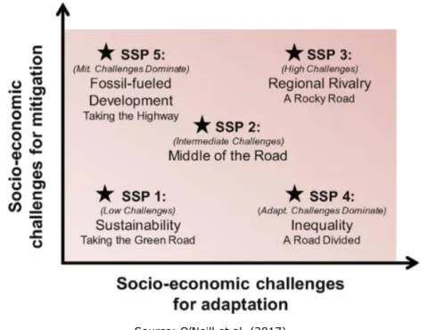
For the agro-economic modelling within the PESETA III project we focus on the SSP2, referred to as “Middle of the Road”. SSP2 represents business as usual development, in which social, economic, and technological trends do not change significantly from historical patterns, i.e. there is some progress towards achieving development goals, reductions in resource and energy intensity at historic rates, and slowly decreasing fossil fuel dependency. This means that population growth, international cooperation, technological growth, convergence between developed and developing countries, and sustainability concerns in consumer behaviour, etc., all show a moderate development path. The moderate development trends in SSP2 imply, on average, rather moderate challenges for mitigation and adaptation of climate change. The positioning of the SSP2 regarding the combination of socio-economic challenges for adaptation and mitigation is depicted in Figure 1.
Figure 1. Different challenges for adaptation and mitigation of climate change in the Shared Socio-economic Pathways
Source: O’Neill et al. (2017)
Regarding the assumptions on economic growth and population, we use the latest population (KC and Lutz 2017) and GDP (Dellink et al. 2017) projections as defined on the basis of a collaborative effort of the international Integrated Assessment Modelling (IAM) community. For SSP2, global population reaches 9.2 billion by 2050, an increase of 35% compared to 2010, and global GDP triples in the same period.
For the parameters translating agricultural sector specific narratives, we interpreted four major land use elements to make them consistent with the general SSP2 narrative: land use change regulation, land productivity growth, environmental impact of food consumption, and international trade. For the interpretation of these narratives in the CAPRI model we follow the same assumptions as used in the AgCLIM50 project (van Meijl et al. 2017). In the following we briefly present these assumptions (for more information see van Meijl et al. 2017).
SSP2 related land use change regulation
Climate change policy is actually not part of the SSPs. Therefore, land use change regulations considered in agro-economic models have a different target, which is usually biodiversity protection, often represented through forest protection measures in the models (van Meijl et al. 2017). In the CAPRI model, improved forest protection is
simulated through a carbon price of 2.5 EUR/t of non-CO2 emissions in agriculture (i.e. methane and nitrous oxide) and in the LULUCF sector5 in SSP2. This carbon price indirectly produces a shift in the use of land from agriculture to other land classes, such as forestry.
SSP2 related crop yield effects
Climate change related crop yield shocks are considered in the agricultural biophysical modelling approach and considered in the CAPRI analysis (see next section). Therefore, crop yield growth could generally be represented as input neutral regarding the SSP2. However, the CAPRI model considers also the relation between yield growth and variable inputs (e.g. use of fertilizers and pesticides), and CAPRI has an exogenous and an endogenous component of yield developments, the latter one triggered by changes in relative prices. Consequently, we also have to consider SSP2 related effects on crop yields for our approach. For the exogenous future crop yields we rely on the GLOBIOM model, which projects future crop yields based on an econometric estimation taking into account the long-term relationship between crop yields and GDP per capita. The yield projections show an average annual increase of 0.60% for SSP2. In CAPRI we implemented 75% of the yield growth estimated for the SSP2 in GLOBIOM. The rationale behind this is that about 25% of the yield growth is already covered endogenously in the CAPRI model. Furthermore, the carbon price mentioned above is implemented, leading as well to endogenous adjustments towards increased fertilizer use efficiency (i.e. the carbon price introduces a cost per emission unit of nitrous oxide, which in turn increases the cost of nitrogen fertilizer use and hence will lead to increased fertilizer use efficiency).
SSP2 related productivity effects in livestock production
Livestock productivity is a more complex concept than crop yields, as it depends (i) on the amount of nutrients needed to produce a unit of output, (ii) on the composition of the feed ratio, and finally (iii) the feed and forage yields in regions where they are produced. For CAPRI we focus here on the first dimension, as feed conversion efficiency is typically the result of an exgenous component, which can be associated, for example, with genetic improvement/breeding, and an endogenous component related to livestock management. Thus, as the carbon price described above (2.5 EUR/t of CO2 equivalents) applies also to direct emissions from agriculture, such as methane from enteric fermentation, this will lead to endogenous adjustments towards increased livestock production efficiency.
SSP2 related effects on food demand
Total food demand is the result of population growth and per capita consumption. In CAPRI, the per capita consumption and the structure of the diet is a function of GDP per capita, prices and preferences. For SSP2, CAPRI uses the default model setup as no change in the structure of the diet is assumed (and GDP and population growth are already SSP2 specific).
SSP2 related effects on international trade
In CAPRI, domestic product preferences are represented by Armington elasticities and no SSP2 specific setup with regard to trade assumptions are applied for SSP2.
5 It has to be noted that in CAPRI the representation of the LULUCF sector is still incomplete for
non-European regions, and hence the LULUCF part was only effective in Europe. However, indirect effects also ensured a curb on agricultural areas outside of Europe that was able to mimic forest protection.
2.4
Climate change scenarios: agricultural biophysical modelling
input for the yield shocks
For the agro-economic analysis within the PESETA III project we mainly focus on the effects of climate change on crop yields. Climate change is projected to affect regional and global crop yields and grassland productivity. There is, however, considerable variation and uncertainty in the projection of biophysical yield changes both in space and time, coming from different climate signals as well as different climate and crop growth models. With respect to climate change related yield shocks in the EU, we rely on input of the agricultural biophysical modelling of Task 3 of the PESETA III project (Toreti et al. 2017). As the agricultural markets are connected via imports and exports on world markets, it is essential for the agro-economic analysis to also consider climate change related yield effects outside the EU. For the respective yield shocks in non-EU countries, we rely on data provided by the AgCLIM50 project (van Meijl et al. 2017). Moreover, we complement EU yield shocks for soybean, rice, and managed grassland with the AgCLIM50 data. The two approaches are described in sections 2.4.2 and 2.4.3, respectively, after a brief outline of the uncertain effects of increased CO2 fertilization on plants (section 2.4.1).
2.4.1
Uncertain effects of elevated atmospheric CO
2concentration on
plants
There is substantial uncertainty on the effect of elevated atmospheric carbon dioxide (CO2) concentration (i.e. enhanced CO2 fertilization) on crop yields, especially in the long run. CO2 is an essential component of the photosynthesis, with the majority of carbon sequestration in commercial food plants occurring through one of two photosynthetic pathways, known as C3 and C4. Much evidence and little uncertainty exists that CO2 fertilization enhances photosynthesis in C3 plants (e.g. wheat, barley, rye, rice, and soybeans) but not in C4 plants (e.g. maize, sorghum, millet, and sugarcane). There is also evidence that increased atmospheric CO2 increases the water use efficiency in all plants (Keenan et al. 2013), which should allow plants to better tolerate hotter and dryer environmental conditions. However, it is much less clear to what extent the increased CO2 fertilization actually translates into higher crop yields (Ainsworth and Long 2005; Gray and Brady 2016), as there are various plant physiological processes that respond to it (Leakey et al. 2009; ), and it may induce a higher susceptibility to invasive insects (Zavala et al. 2008) and the loss of desirable plant traits (Ribeiro et al. 2012). Moreover, increased CO2 fertilization may reduce the concentration of protein and essential minerals (iron and zinc) in key food crops and hence have negative effects on their nutritional value (Myers et al. 2014). Due to the many complex interaction mechanisms, the effect of increased atmospheric CO2 concentration is still very uncertain and broadly discussed in the research community (Long et al. 2006; Tubiello et al 2007; Wang et al. 2012; Boote et al. 2013; Nowak 2017; Obermeier et al. 2017). As a consequence, future projections of crop yields under climate change and the associated elevated atmospheric CO2 concentrations are often conducted for two scenarios, and we follow this approach also in the study at hand. One scenario assumes that the stimulation of photosynthesis can be translated into higher yields in the long term (indicated in our scenario runs as "_CO2"), and one scenario assumes that there is no long-term benefit of CO2 fertilization ("_noCO2"), which is typically implemented in models by running the models with constant CO2 concentrations (see e.g. Rosenzweig et al. 2014).
2.4.2
Biophysical yield shocks in the EU
For the climate change related yield shocks in the EU, we use the crop yields simulated in Task 3 of the PESETA III project (Toreti et al. 2017). In Task 3, crop growth model runs have been performed based on downscaled and bias-corrected RCP8.5 regional climate model (RCM) runs from the Coordinated Regional Downscaling Experiment for Europe
(EURO-CORDEX)6, as defined in Task 1 of PESETA III. In Task 1 of PESETA III, five runs were selected and bias-corrected by using the quantile mapping approach (Dosio, 2017). For the crop growth model simulations the BioMA modelling framework was used. The EU-wide yield shocks at national and NUTS2 level provided to this Task are based on crop yield simulations under water-limited conditions7 with and without increased CO
2 levels for the following six crops: winter wheat, spring barley, grain maize, sugar beet, winter rapeseed, and sunflower. CAPRI covers more disaggregated crops than the six crops covered by Task 3, and we therefore assume that similar crops have the same yield change as the ones specifically provided. For some crops, like for example fruits and vegetables, an aggregated change in yields is assumed.
The yield shocks were derived as the difference in simulated yields for 2050 and the baseline; both time horizons are defined as 30-year averages of the transient simulations of 2036 to 2065 and 1981 to 2010, respectively. The average of 30 years is taken in order to get a climatological value, averaging out the noise of varying weather in single years. Furthermore, the yield changes have been averaged over all five RCP8.5 climate simulations chosen for PESETA III as defined in Task 1 (i.e. ID-1 to ID-5). In Task 3 of the PESETA III project, the MARS Crop Yield Forecasting System (MCYFS) database was taken for the parameterization of different crops and their spatial distribution, assuming that the crop varieties remain constant in time. The Crop Growth Monitoring System (CGMS) soil database (Baruth et al. 2006) was used to derive gridded soil data and for each land grid cell of the EURO-CORDEX domain the dominant soil type was chosen. Further details on the biophysical simulations and the climate change related yield shocks in the EU can be found in the description of Task 3 of the PESETA III project (Toreti et al. 2017).
2.4.3
Complementing biophysical yield shocks (in EU and non-EU
countries)
The agricultural biophysical modelling in PESETA III only focuses on the above mentioned climate change related yield shocks in the EU. However, for the analysis of agro-economic impacts it is crucial to consider also climate change related yield shocks in non-EU countries, as agricultural markets are interrelated via international imports and exports that determine the impact on regional agricultural prices and income. Therefore it was necessary to use a second source that depicts the climate change related yield shocks in non-EU countries. Even though EU and non-EU yield shocks rely on (similar but) slightly different agricultural biophysical modelling runs, and hence our approach might not be totally consistent, this inconsistency was considered better than ignoring climate change effects in non-EU countries, as it could have led to a seriously under- or overestimation of the impacts.
For the non-EU yield shocks, we rely on information gathered within the AgCLIM50 project (van Meijl et al. 2017), which comprises a representative selection of climate change impact scenarios on crop yields. The selection is based on multiple available combinations of results from Global Gridded Crop Growth Models (GGCM) and General Circulation Models (GCM) for the selected RCP8.5. For the use in the CAPRI model, results from global gridded crop models are aggregated to the country level. The Inter-Sectoral Impact Model Intercomparison Project (ISI-MIP) fast-track data archive (Warszawski et al. 2014), provides data on climate change impacts on crop yields from seven global GGCMs (Rosenzweig et al. 2014) for 20 climate scenarios. The climate scenarios are bias-corrected implementations (Hempel et al. 2013) of the four RCP by five GCM8 from the Coupled Model Inter-comparison Project (CMIP5) data archive (Taylor et al. 2012). Within AgCLIM50, three GGCM have been selected based on data
6 For more information see: http://www.euro-cordex.net
7 Water-limited production levels account for the impact of a limited water supply and hence water stress on
biomass accumulation. This production level is especially important to assess the response of rain-fed crops.
8 The five GCMs are: HADGEM2-ES, IPSL-CM5A-LR, MIROC-ESM-CHEM, GFDL-ESM2M, NorESM1-M (van Meijl
availability: EPIC (Williams 1995), LPJmL (Bondeau et al. 2007; Müller and Robertson 2014), pDSSAT (Jones et al. 2003; Elliott et al. 2014). Accordingly, there were 15 scenarios available for RCP8.5, and hence the selection of representative scenarios is based on 15 GGCM x GCM combinations for the assumption with and without CO2 fertilization (for further explanation see van Meijl et al. 2017).
From the 15 GGCM x GCM combinations, we use the "median" combination for the further analysis in CAPRI, i.e. the one that represents the global median impact, for the RCP8.5 and each assumption on CO2 fertilization. The selection of the median avoids the extreme bias of selecting pixel- or region-based values from that unit’s impact distribution and keeps spatial consistency in impacts. For the mapping of crops simulated in the GGCM to commodities used in the CAPRI model, the same mechanism as in Nelson et al. (2014) was applied. Variations in non-EU yields are supplied by GGCM as annualized growth rates from 2000 (1986-2015 average) to 2050 (2036-2065 average) at the country level. Data was supplied at country level for the four major crops (wheat, maize, rice and soybean) and managed grassland.
In practice this means that for biophysical yield shocks in EU countries we use the ones provided by Task 3 of the PESETA III project for wheat, barley, grain maize, sugar beet, rapeseed, and sunflower as well as the ones provided within the AgCLIM50 project for soybean, rice and grassland. For the biophysical yield shocks in non-EU countries we use the ones provided by the AgCLIM50 project for wheat, maize, rice, soybean, and managed grassland. For all other crops the effect of climate change on yields is assumed to be the average of the effects for wheat, barley and grain maize for other cereals (e.g. rye) and the average of all for the rest of the crops (e.g. fruits and vegetables). These assumptions are needed since no specific biophysical yield responses to climate change are provided by biophysical models for these crops, and in order to avoid unlikely cross-effects between crops affected and not affected by climate change (e.g. expansion of rye production due to a reduction in wheat yields).
3
Scenario results
The scenario results are the outcome of the simultaneous interplay of the SSP2 narrative, climate change related biophysical yield shocks in the EU and non-EU countries as introduced based on the interactions between global climate and crop growth models, and the induced and related effects on agricultural production, trade, consumption, and prices at domestic and international markets.9 In this chapter we present the results of two climate change scenario variants for a RCP of 8.5 W/m2 (i.e. a scenario of comparatively high GHG emissions), without enhanced CO2 fertilization (RCP8.5_noCO2) and with enhanced CO2 fertilization (RCP8.5_CO2), with respect to impacts on agricultural production, trade, prices, consumption, income, and welfare in the EU. Both scenarios are compared to the Reference Scenario (REF2050), which represents the counterfactual situation with no climate change considered. The projection horizon for all scenarios is 2050.
3.1
Impact on agricultural production
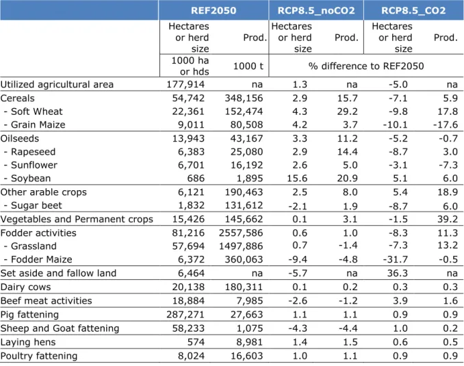
The impact of climate change on EU-28 production aggregates in 2050 compared to production without climate change (REF2050 scenario) is depicted in Table 1. Production effects at EU Member States and regional levels are presented further down below. The production presented is accounting for both the direct changes in yield and area caused by climate change and autonomous adaptation as farmers respond to changing prices with changes in the crop mix and input use.
As can be seen in Table 1, results differ quite significantly depending on whether enhanced CO2 fertilization is assumed or not. For the scenario RCP8.5_noCO2, climate change related effects are mainly visible in the crop sector and generally positive at the aggregated EU level, with increases in both hectares and production. The increase in production10 is larger than the increase in hectares under production, which is mainly debited to a positive net effect of climate change on EU crop yields in the main production regions, but also due to favourable market conditions that support EU net exports (i.e. more adverse effects on average in non-EU crop production regions). For example, as a result of both the exogenous (biophysical) climate change induced yield shocks and the endogenous market related yield adjustments, average cereals yields in the EU increase by more than 12% compared to the REF2050 scenario. A general net increase in aggregated yields and hence EU production can well be observed in all other crop related activities, including oilseeds, other arable crops (mainly sugar beet, pulses and potatoes), as well as fruits and vegetables. With increasing area for nearly all crops, the area for set aside and fallow land is reduced by almost 6% and also total utilized agricultural area (UAA) increases by about 1%. In the livestock sector, a decrease is shown for activities related to ruminant meat production, with drops in herd size and production for beef meat activities and sheep and goat fattening. This can be attributed to a climate change induced decrease in grassland and fodder maize production, the main feed for ruminant production. On the other hand, pork and poultry are less negatively affected and see (slight) production increases, which partly compensates for the decrease of ruminant meat production.
When enhanced CO2 fertilization is assumed (RCP8.5_CO2), increasing production output with decreasing area in the crop sector indicate the, on average, stronger (and more positive) EU biophysical yield shocks compared to the scenario without CO2 fertilization (RCP8.5_noCO2). The land devoted to cereals shows a decrease of -7%, but production still increases by +6% compared to the REF2050 scenario. However, regarding cereals it is especially important to distinguish between the effects on wheat (a C3 plant) and maize (a C4 plant) in this scenario. Although area drops for both crops by -10%, the final production adjustment is positive for aggregated EU wheat production
9 In the final equilibrium, prices change in all EU and non-EU regions, triggering endogenous adjustments of
crop yields, such that the final yield changes differ from the exogenously implemented productivity shocks.
(+18%), but negative for maize (-18%). This reflects the positive effect of enhanced CO2 fertilization on EU biophysical wheat yields, which is not given (or negative) regarding maize yields in several MS. Oilseeds production slightly drops on average, owing to a -7% decrease in EU sunflower production compared to REF2050, as rapeseed and soybean production are increasing by +3% and +6%, respectively. An increase in yields is also evident in fodder activities, mainly grassland, which show an increase in production of 11% despite a drop in area of -8%. The net effect of the area and production developments is a decrease of -5% in total EU UAA, but also a considerable increase in area of set aside and fallow land (+36%). The EU livestock sector benefits from the further enhanced cereals and grassland yields, especially due to lower prices for animal feed (as will be shown in the next sections), leading to (slight) increases in both animal numbers and production for ruminant and non-ruminant production.
Table 1. Change in EU-28 area, herd size and production compared to REF2050 REF2050 RCP8.5_noCO2 RCP8.5_CO2 Hectares
or herd size
Prod. Hectares or herd size
Prod. Hectares or herd size
Prod. 1000 ha
or hds 1000 t % difference to REF2050
Utilized agricultural area 177,914 na 1.3 na -5.0 na
Cereals 54,742 348,156 2.9 15.7 -7.1 5.9 - Soft Wheat 22,361 152,474 4.3 29.2 -9.8 17.8 - Grain Maize 9,011 80,508 4.2 3.7 -10.1 -17.6 Oilseeds 13,943 43,167 3.3 11.2 -5.2 -0.7 - Rapeseed 6,383 25,080 2.9 14.4 -8.7 3.0 - Sunflower 6,701 16,192 2.6 5.0 -3.1 -7.3 - Soybean 686 1,895 15.6 20.9 5.1 6.0
Other arable crops 6,121 190,463 2.5 8.0 5.4 18.9
- Sugar beet 1,832 131,612 -2.1 1.9 -8.7 6.0
Vegetables and Permanent crops 15,426 145,662 0.1 3.1 -1.5 39.2
Fodder activities 81,216 2557,586 0.6 1.0 -8.3 11.3
- Grassland 57,694 1497,886 0.7 -1.4 -7.3 13.2
- Fodder Maize 6,372 360,063 -9.4 -4.8 -31.7 -0.5
Set aside and fallow land 6,464 na -5.7 na 36.3 na
Dairy cows 20,138 180,311 0.1 0.2 0.3 0.3
Beef meat activities 18,884 7,985 -2.6 -1.2 3.9 1.6
Pig fattening 287,271 27,663 1.1 1.1 0.9 0.9
Sheep and Goat fattening 58,233 1,075 -4.3 -4.4 1.0 0.2
Laying hens 574 8,981 1.4 1.5 0.6 0.5
Poultry fattening 8,024 16,603 1.0 1.1 0.9 0.9
Note: Prod. = production; na = not applicable; total production of beef includes beef from suckler cows, heifers, bulls, dairy cows and calves
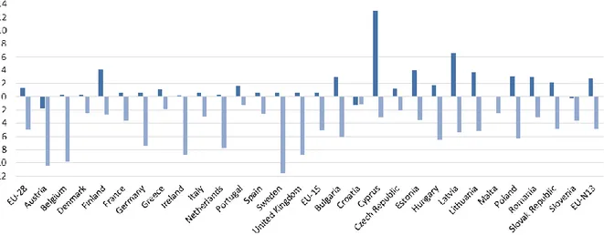
Production effects at EU MS and regional levels reveal that almost all Member States show the same trend as indicated for the aggregated EU-28. Notwithstanding, regional differences can be quite significant. Figure 2 and Figure 3 present the case of UAA at MS and regional level. While aggregated EU UAA increases in the RCP8.5_noCO2 scenario by more than +1%, scenario RCP8.5_CO2 shows a decrease in EU UAA of -5%. With the exception of Austria (-1.7%) and Croatia (-1.2%), UAA increases also in all Member States in scenario RCP8.5_noCO2, and UAA decreases in all Member States in scenario RCP8.5_CO2. In scenario RCP8.5_noCO2, UAA shows the highest relative increase in Cyprus, but in absolute terms the increase is biggest in Poland (+0.5 mio ha) and Romania (+0.4 mio ha). For scenario RCP8.5_CO2, Sweden, Austria and Belgium show
the biggest relative decrease in UAA, but the absolute decreases are highest in the UK, Germany, Poland and France (each with decreases of more than 1 mio ha). The relative changes in UAA at regional level are shown in Figure 3, reflecting the effects at EU NUTS 2 level.
Figure 2. Percentage change in UAA (hectares) relative to REF2050, EU Member States
Figure 3. Percentage change in UAA (hectares) relative to REF2050, EU NUTS 2 regions, scenarios RCP8.5_noCO2 (left) and RCP8.5_CO2 (right)
A closer look at cereals production
In the following we take the example of cereals production to show how the combined effects of climate change and market-driven changes translate into the area, yield and production adjustments. As the aggregated cereals results hide large differences of climate change impacts on yields of different cereals, we also have a closer look at the market-adjusted impacts on wheat and grain maize production.
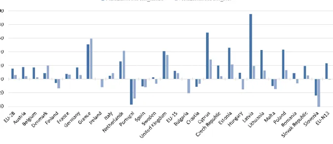
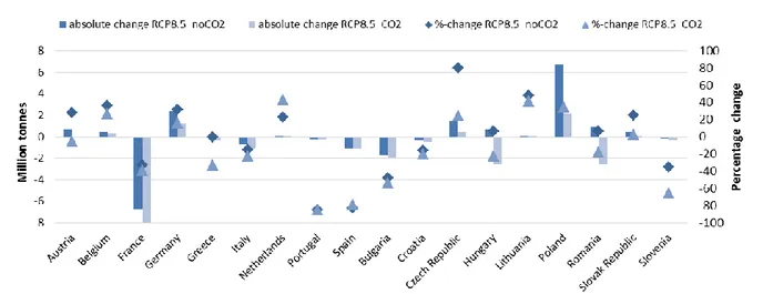
Figure 4 and Figure 5 present percentage changes in cereals production at EU Member State and regional level for both climate change scenarios relative to REF2050. As outlined above, if a Member States indicates a reduction in cereals production, this is not necessarily (only) due to climate change induced negative biophysical yield shocks, but also due to agricultural market developments (prices, trade, etc., see below). Figure 4
indicates a positive effect in the RCP8.5_noCO2 scenario on cereals production in almost all Member States. When looking at the figure it has to be kept in mind that in some Member States cereals production is rather small, which is why relative changes can be quite high even though they are rather small in absolute terms (as for example in Cyprus and Latvia). Considering absolute terms, the production changes are particularly relevant in Poland (+43%), UK (41%), Germany (+17%) and France (+8%). Six Member States show a decrease in cereals production, of which in absolute terms especially the reduction in Spain (-11%) is considerable. In the scenario RCP8.5_CO2, positive effects on cereals production are generally less pronounced, and the number of Member States that are negatively affected increases to 11.
Figure 4. Percentage change in cereals production relative to REF2050, EU Member States
Figure 5. Percentage change in cereals production relative to REF2050, EU NUTS-2 regions, scenarios RCP8.5_noCO2 (left) and RCP8.5_CO2 (right)
When looking at the results of cereals production, it is especially important to keep in mind that the aggregated cereals results hide large differences between the impacts on different cereals, as, for example, wheat and grain maize. To better represent the impact of climate change on wheat and grain maize yields, we first show the implemented biophysical yield shocks for both crops in the following four figures and then show their respective yields after the market-driven adjustments. It can be noted that especially
Figure 7 shows the disadvantage of using the input of different climate and biophysical models for EU and non-EU countries, as the changes in biophysical wheat yields in the EU under the assumptions of elevated CO2 fertilization seem somewhat too optimistic compared to non-EU countries.
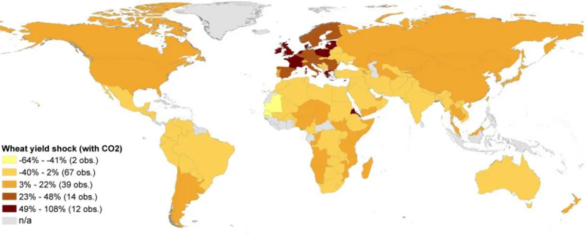
Figure 6. Biophysical wheat yield shocks in the RCP8.5_noCO2 scenario
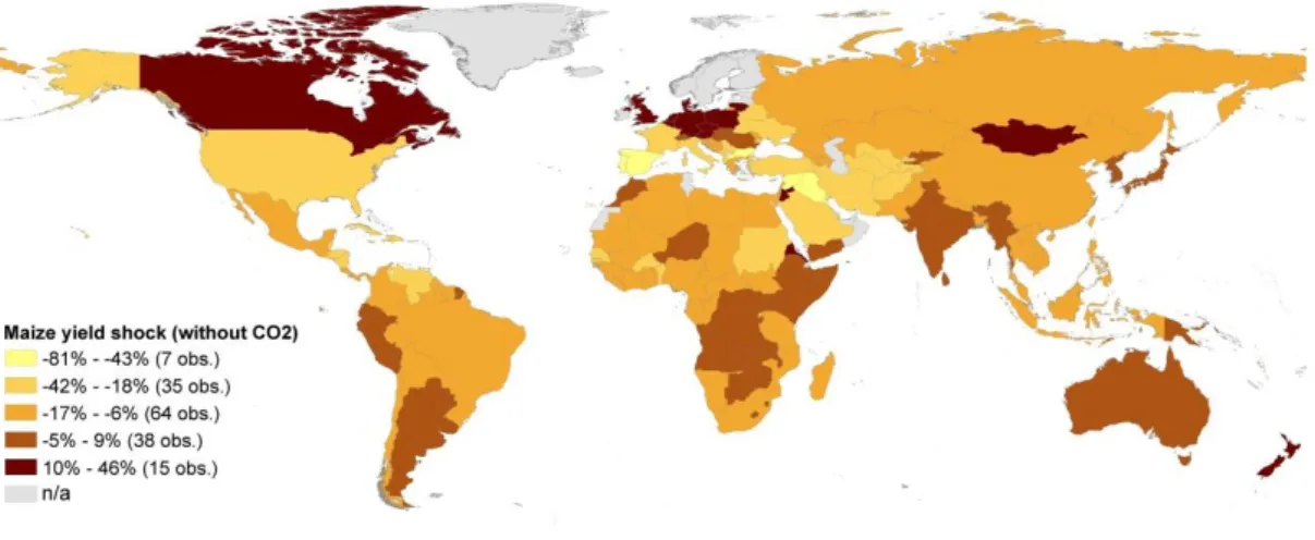
Figure 8. Biophysical grain maize yield shocks in the RCP8.5_noCO2 scenario
Figure 9. Biophysical grain maize yield shocks in the RCP8.5_CO2 scenario
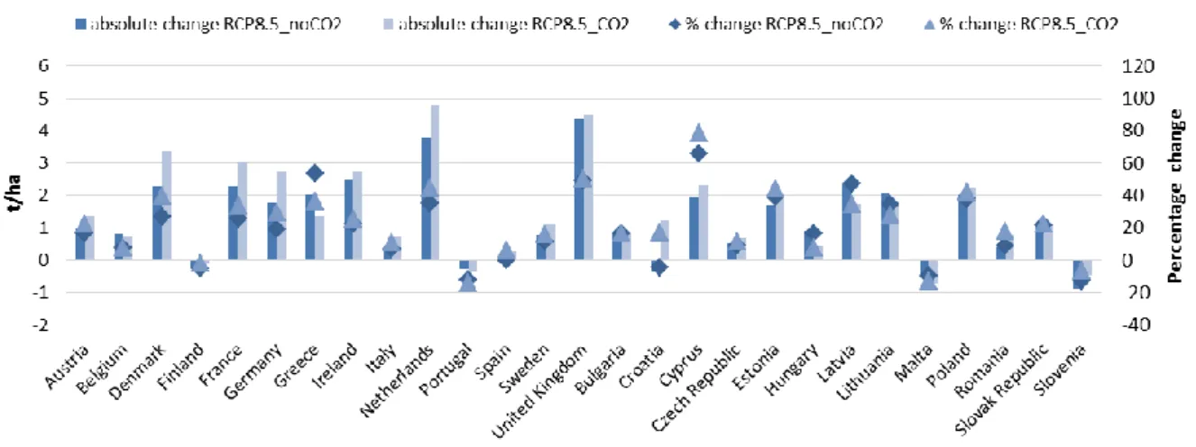
Figure 10 shows the absolute and percentage change in soft wheat yields in the two climate change scenarios at EU Member State level relative to REF2050 following market-driven adjustments. The indicated change in wheat yield is an outcome of the combination of climate change related biophysical yield shocks that have been exogenously introduced into the CAPRI model based on the agro-biophysical modelling results (see section 2) and the endogenous yield adjustments calculated by the CAPRI model following commodity market-driven adjustments. The biophysical yield shock is actually positive for all MS except for Croatia, Portugal and Slovenia in the RCP8.5_noCO2 scenario, and even more positive for all MS when enhanced CO2 fertilization is assumed (turning into a positive effect also in the three MS indicated above). Our scenario results show that also after the market adjustments, the net yield effect is positive at aggregated EU-28 level, with wheat yields increasing by 24% in the RCP8.5_noCO2 scenario and by more than 30% in the scenario RCP8.5_CO2. The results are diverse between the two scenario variants, but in most Member States the net effect of an enhanced CO2 fertilization on wheat yield is positive, i.e. yields improve compared to RCP8.5_noCO2, with the exception of Portugal, Malta, Greece, Hungary, Latvia, Lithuania and Belgium. In absolute terms, the final yield changes are most important in the UK and the Netherlands. These results demonstrate the importance of taking market-driven effects into account, as the biophysical yield effect is actually positive for all EU MS, and if only EU production and no interrelation with world market developments would be
considered, wheat yields would increase in all EU Member States in the RCP8.5_CO2 scenario compared to both the RCP8.5_noCO2 scenario and the REF2050 scenario.11
Figure 10. Absolute and percentage change in soft wheat yields (considering climate change + market adjustments) compared to REF2050, EU Member States
Even though average EU wheat yields increase more under the assumption of enhanced CO2 fertilization, the total increase in EU wheat production is lower in the RCP8.5_CO2 scenario (+18%) than in the RCP8.5_noCO2 scenario (almost +30%) - which is due to the 10% decrease in EU wheat area following higher competition on international markets (see below in the following chapters). Accordingly, only Denmark, the Netherlands and Croatia show a higher total wheat production in RCP8.5_CO2 compared to the RCP8.5_noCO2 scenario (Figure 11). In scenario RCP8.5_noCO2, most countries (Figure 11) and regions (Figure 12) in Southern Europe show a drop in wheat production, whereas especially regions in Northern France, Central Europe North and Northern Europe benefit from climate change induced production increases. Biggest absolute production increases are projected for France and the UK (above 10 million tonnes each), Poland (+6 mio t), Germany (+5.7 mio t), Latvia (+3 mio t) and Lithuania (+2.7 mio t).
Figure 11. Absolute and percentage change in soft wheat production compared to REF2050, EU Member States
11 This was tested with auxiliary scenarios where only EU production and no interrelation with the world
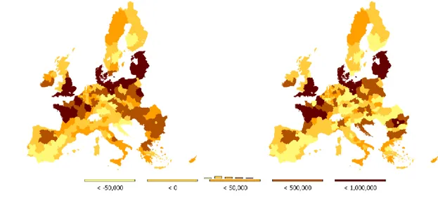
Figure 12. Absolute change in soft wheat production compared to REF2050 (1000 t), EU NUTS-2 regions, scenarios RCP8.5_noCO2 (left) and RCP8.5_CO2 (right)
Figure 13 presents the percentage changes in grain maize yields at EU Member State level relative to REF2050. In both climate change scenarios, the net effect of climate change on grain maize yields (i.e. after market-driven adjustments) is negative at aggregated EU level, -0.5% in RCP8.5_noCO2 scenario and -8% in scenario RCP8.5_CO2. The yield effect is diverse across countries, and again, there is a difference in the pattern between the two scenarios regarding the biophysical yield shocks and the final yields obtained after the market-driven adjustments: (1) regarding pure biophysical yield shocks, positive yield effects are more, and negative effects less pronounced in the scenario assuming enhanced CO2 fertilization; whereas (2) regarding end yields after the market-driven adjustments, positive yield effects are generally less, and negative effects more pronounced in the scenario assuming enhanced CO2 fertilization. In both scenarios, final maize yields are most negatively affected in Portugal, Spain, Bulgaria, France, and Slovenia. The differences between the pattern of biophysical yield shocks and final yields obtained after market-driven adjustments in scenario RCP8.5_noCO2 can mainly be explained by reduced market competiveness of EU grain maize production compared to non-EU countries (trade effect) as well as compared to wheat production (production-mix effect).
Figure 13. Absolute and percentage change in grain maize yields (considering climate change + market adjustments) compared to REF2050, EU Member States
Figure 14 shows that in scenario RCP8.5_noCO2, despite the slight decrease in EU average grain maize yields, total EU grain maize production increases by 3.7%, which is due to an increase of the respective area by 4.2%. In scenario RCP8.5_CO2, EU grain maize production shows a drop of almost 18%, which apart from the decrease in average yield (-8%) is also due to the decrease in area (-10%). In both scenarios, France remains the biggest grain maize producer in the EU, but it is also the most negatively affected MS in terms of absolute production decreases (-6.7 mio t in RCP8.5_noCO2, -8 mio t in RCP8.5_CO2), because farmers lose competitiveness due to the exogenous negative climate change yield shocks. The absolute production decrease is also considerable in Bulgaria, Spain and Italy in both scenario variants and in Hungary and Romania in scenario RCP8.5_CO2. Except the latter two, all countries that show a considerable decrease in grain maize production are affected by a negative exogenous yield shock. Accordingly, the production decreases in Hungary and Romania are market-driven, i.e. adjustments due to market price changes etc. (see sections below).
The most positive affected MS in terms of absolute production increase in scenario RCP8.5_noCO2 are Poland (+6.7 mio t), Germany (+2.4 mio t), and Czech Republic (+1.5 mio t). The grain maize production in these three MS also benefits most from climate change when enhanced CO2 fertilization is assumed, but the absolute production increase is considerable less than in scenario RCP8.5_noCO2.
Figure 14. Absolute and percentage change in grain maize production compared to REF2050, EU Member States
Note: Member States not indicated do not have (a relevant) grain maize production
3.2
Impact on agricultural trade
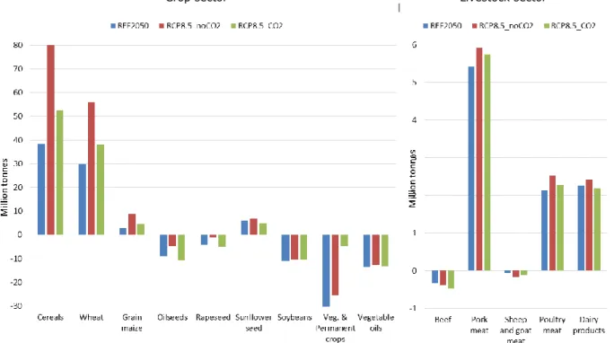
The EU's agricultural trade balance (exports - imports) reflects the production effects indicated in section 3.1. As shown in Figure 15, in both scenario variants the EU trade balance improves for almost all agricultural commodities, except for beef, sheep and goat meat (and oilseeds production in scenario RCP8.5_CO2). EU cereals exports are especially positive affected in the Scenario RCP8.5_noCO2, showing an increase of 81% (imports also decrease by 78%, but the quantities involved are much smaller). As indicated already in section 3.1 with respect to production, the EU cereals trade balance also improves in Scenario RCP8.5_CO2, but less than in the scenario without enhanced CO2 fertilization, with an increase in exports of 25% and a decrease in imports of 43% compared to REF2050. Accordingly, the EU share in world cereals exports increases from 19% in REF2050 to 29% in Scenario RCP8.5_noCO2 and 21% in Scenario RCP8.5_CO2. As a result of the changes in domestic production and the trade balance, EU net trade relative to the average market volume increases from 11% in REF2050 to 20% in Scenario RCP8.5_noCO2 and 14.5% in Scenario RCP8.5_CO2 (Table 2). That the EU
cereals exports do not increase more in Scenario RCP8.5_CO2 compared to RCP8.5_noCO2 is because several non-EU countries also experience considerable production increases under the assumption of enhanced CO2 fertilization, which in turn increases either their export potential or decreases their need for imports, and leads to augmented competition on the world market (Table 2).
The EU trade balance for oilseeds improves in scenario RCP8.5_noCO2 compared to REF2050, but worsens in the scenario RCP8.5_CO2, basically reflecting the domestic production developments in the two scenario variants. The EU production increase in vegetables and permanent crops is also well reflected in the EU trade balance, which, due to both increasing exports and decreasing imports, improves from REF2050 to RCP8.5_noCO2 and considerably more when enhanced CO2 fertilization is assumed. For the EU livestock sector, the domestic production increases in pig and poultry fattening lead to increasing EU exports in both scenario variants, further improving the respective EU net exporter positions. However, the increase in ruminant meat production in scenario RCP8.5_CO2 does not lead to an improvement of the EU trade balance compared to REF2050, which is due to an increase of relatively cheaper imports (Figure 15).
Figure 15. EU trade balance in the scenarios (2050)
Crop sector Livestock sector
Note: Trade balance = exports – imports; cereals = the aggregate of wheat, grain maize, and other cereals; oilseeds = the aggregate of rapeseed, sunflower, and soybeans.
Table 2. Agricultural trade indicators cereals
Note: Net trade = exports – imports.
REF2050 RCP8.5_noCO2 RCP8.5_CO2
Net Trade Net Trade relative to average market volume World Export share World Import share Net Trade Net Trade relative to average market volume World Export share World Import share Net Trade Net Trade relative to average market volume World Export share World Import share 1000 t % % % 1000 t % % % 1000 t % % % EU-28 38426 10.9 19.3 8.7 80271 20.1 29.1 7.6 52567 14.5 20.6 6.3 Europe, Non-EU 39833 14.4 14.5 3.5 36155 13.3 13.1 3.4 41898 14.8 15.4 4.1 - Russia 7223 6.2 2.2 0.3 797 0.7 1.0 0.8 5887 5.0 1.9 0.3 - Ukraine 10428 22.4 3.2 0.3 10523 22.6 3.1 0.3 7872 17.5 2.5 0.3 North America
(USA, CAN, MEX) 44572 4.8 36.6 24.4 8070 1.0 26.0 23.9 45341 4.8 36.1 23.8
- USA 78920 10.7 25.9 4.3 43057 6.9 18.2 6.7 73388 9.8 24.5 4.5
- Canada 23569 28.1 10.4 4.0 15338 21.3 7.7 3.6 29372 32.8 11.4 3.4
Middle and South
America 32049 12.6 16.9 8.1 39722 15.1 19.1 8.5 25476 10.4 14.7 7.7
- Brazil 2478 2.2 2.3 1.7 2368 2.1 2.4 1.8 -1215 -1.1 1.7 2.0
- Argentina 42621 62.7 11.7 0 50349 66.9 13.5 0 39349 60.8 10.7 0
Africa -77643 -21.6 1.1 22.4 -81237 -22.4 1.6 23.3 -78210 -21.4 3.0 24.3
Asia -98703 -11.0 5.8 32.8 -105479 -12 5.0 33.2 -105629 -11.8 5.1 33.8
Australia & New
Zealand 21546 48.2 5.9 0 22564 49.2 6.0 0 18619 44.7 5.1 0
High income 21362 2.1 42.8 36.9 -13503 -1.5 32.4 36.0 19228 1.9 41.4 36.2
Middle income -50692 -4.1 21.6 35.5 -61006 -5.1 19.7 36.0 -56685 -4.6 21.5 36.9
3.3
Impact on EU agricultural prices and income
Prices are a useful indicator for the economic effects of climate change on EU agriculture. Figure 16 shows the effects of the two climate change scenarios on agricultural producer and consumer prices in the EU, without (RCP8.5_noCO2) and with (RCP8.5_CO2) enhanced CO2 fertilization. In general, climate change leads to decreases for EU agricultural crop prices in both scenario variants. The livestock sector is not directly affected by climate change in the model runs, but the effects on feed prices and trade caused by climate change pass through to prices of livestock products.
In the scenario RCP8.5_noCO2, aggregated crop producer price changes vary between -3% for cereals (-7.5% for wheat) and +5% for other arable field crops (e.g. pulses and sugar beet), whereas producer price changes in the livestock sector vary between -6% for sheep and goat meat, and +4% for pork meat. Interestingly, pork and poultry producers benefit from price increases mainly due to a favourable export environment (i.e. exports increase), whereas the producer price decrease for ruminant meats is mainly due to an increase in relatively cheaper imports, which more than offset the respective EU production decrease provoked by the rise in ruminant related feed prices. Following the production increases and changes in the trade balance in scenario RCP8.5_CO2, agricultural producer prices in the EU decrease for all commodities, not only compared to REF2050, but also compared to scenario RCP8.5_noCO2. This is due to the general increase in domestic production, which, compared to REF2050 and the scenario without enhanced CO2 fertilization, faces a tougher competition on the world markets, consequently leading to decreases in producer prices. Accordingly, EU producer prices in the crop sector drop between -20% for cereals (-25% for wheat) and almost -50% for vegetables and permanent crops in scenario RCP8.5_CO2 compared to REF2050. In the livestock sector, producer price changes are less pronounced, but prices still decrease between -7.5% for cow milk and -19% for beef meat as livestock benefits from cheaper feed prices (and producer prices are further subdued due to increased imports).
Consumer prices follow the developments of producer prices in both scenario variants, but due to high consumer margins (assumed constant), the relative changes are much lower. Nonetheless, in scenario RCP8.5_CO2, the decrease in consumer prices is remarkable for fruits and vegetables, and for ruminant meats.
Figure 16. Percentage change in EU producer and consumer prices relative to REF2050
3.4
Impact on EU consumption
Agricultural output used for human consumption is determined by the interaction of production, demand, and the resulting prices with individual preferences and income. In general, the EU consumption changes provoked by the modelled climate change are of relatively lower magnitude and basically follow the above indicated changes in consumer prices. In the scenario RCP8.5_noCO2, fruits and vegetable consumption is increasing by about 1%, whereas meat consumption is declining by -0.5% compared to the REF2050 scenario. However, while beef, pork and poultry meat consumption is reduced, consumption of sheep and goat meat is increasing due to the relatively bigger decrease in consumer prices of the latter compared to beef meat and the increasing prices for pork and poultry. In scenario RCP8.5_CO2, the considerable price decrease for fruits and vegetables leads to a high consumption increase of almost 13%. Even though consumer prices decrease for all meats, pork and poultry consumption decline whereas beef (+2.6%) and sheep and goat meat (5.2%) consumption rises, as the latter two become relatively cheaper compared to the former two meats. Total dairy consumption is slightly decreasing (-0.2%), but the consumption of higher value cheese slightly increases (+0.5%).
Figure 17. Percentage change in EU consumption relative to REF2050
3.5
Impact on EU agricultural income and welfare
The combination of the above outlined changes in production, trade, prices, and consumption affect total agricultural income in the EU. Total agricultural income takes into account the changes in the product margins (gross added value - cost) and in the production quantity of all agricultural activities. The effect on total agricultural income at aggregated EU-28 level is positive in the scenario without enhanced CO2 fertilization, showing an increase of 5%, whereas a decrease in total agricultural income of 16% is projected when enhanced CO2 fertilization is considered.
The variance in agricultural income change is quite strong at MS and regional level. In scenario RCP8.5_noCO2, six MS show a negative income development (Italy, Greece, Croatia, Malta, Slovenia, Finland), but about two-thirds of all NUTS2 regions experience an income increase. In scenario RCP8.5_CO2, only four MS indicate an income increase (Netherlands, UK, Poland, Cyprus), whereas about 90% of the NUTS2 regions experience a reduction of income. The impact of climate change on total agricultural income by NUTS2 region is shown in Figure 18. As can be seen, the impact varies considerably between the regions, but as a general rule, almost all EU regions are negatively affected in the scenario with CO2 fertilization.