ELECTRE TRI for Groups with Imprecise Information on Parameter Values

ELECTRE TRI for Groups with Imprecise Information

on Parameter Values

LUIS C. DIAS

Faculty of Economics, University of Coimbra, Av. Dias da Silva 165, 3004-512 Coimbra, Portugal and INESC, R. Antero de Quental 199, 3000-033 Coimbra, Portugal, Tel. +351 239 832689

JOÃO N. CLÍMACO

Faculty of Economics, University of Coimbra, Av. Dias da Silva 165, 3004-512 Coimbra, Portugal and INESC, R. Antero de Quental 199, 3000-033 Coimbra, Portugal, Tel. +351 239 832689

Abstract

ELECTRE TRI is a well-known method to assign actions to predefined ordered categories, considering multiple criteria. Using this method requires setting many parameters, which is often a difficult task. We consider the case where a group of Decision Makers (DMs) is unsure of which values each parameter should take, which may result from insufficient, imprecise or contradictory information, as well as from lack of consensus among the group members. In a framework where DMs provide constraints bounding and interrelating the parameter values, rather than fixing precise figures, we discuss the problem of finding the best and worst category that each action may attain.

Key words: ELECTRE TRI, decision by consensus, imprecise/partial information, robustness analysis

1. Introduction

ELECTRE TRI (Yu, 1992) is a well-known approach to decision aid when there is a discrete set of actions a₁, ..., a_m (e.g. investment projects) to be assigned to a set of ordered categories (e.g. “reject”, “accept if ...”, “accept as is”), according to multiple criteria. This method builds a fuzzy outranking relation (Roy, 1991) and then exploits it for decision aid (see description in Section 3). Decision Makers (DMs) have to set the performance of each action on each criterion, the thresholds that characterize pseudo-criteria, the importance and veto power of each criterion plus a cut threshold that is used to transform the resulting fuzzy relation into a crisp one, all of which constitute the model’s parameters. We refer to parameters in a broad sense, including input usually referred to as “data”, input concerning the DMs’ values and beliefs, etc.

Given a numerical value for each parameter, the pessimistic or optimistic ELECTRE TRI assigns each action to a well-determined category. However, it is unrealistic to expect that DMs are able to agree on the values for the parameters, since (see also on this subject Roy and Bouyssou, 1989; French, 1995):

– the performance of each action on each criterion may be unknown at the time of the analysis (uncertainty concerning the future), it may result from aggregating several

aspects with impact on the criterion (arbitrariness in constructing parts of the model), and it may result from a measuring instrument or a statistic measure (which usually involve imprecision);

– parameters such as the importance coefficients and veto thresholds have no objective existence (independent from the method): they reflect the DMs’ subjective values, which they may find difficult to express and that may change over time;

– in either case, the DMs may not entirely agree on the values that each parameter should take, due to different opinions (perceptions) and values (preferences). We consider a group decision setting where multiple instances of a model (each one corresponding to an admissible combination of values for the parameters) are accepted. The multiple instances are expressed as a set of constraints, rather than a discrete set of values. The constraints may be explicitly provided by the DMs or inferred from holistic comparisons (as in Mousseau, 1993). Although constraints are not always easy to provide, requiring precise values for the parameters is obviously more demanding. We consider the use of our approach to be an interactive learning process, where the results of the analysis may stimulate the DMs to discuss and revise their inputs.

The information leading to the set of constraints is often called “imprecise” (e.g. Athanassopoulos and Podinovski, 1997), “incomplete” (e.g. Kim and Ahn, 1997), “partial” (e.g. Hazen, 1986) or “poor” (e.g. Bana e Costa and Vincke, 1995). We will use the expression “imprecise information”, meaning that it does not impose a precise combination of values for the parameters, which also allows coping with insufficient or contradictory information.

Let T represent the set of all acceptable combinations of parameter values. This set could be either the intersection or the union of the combinations of values accepted by each individual DM, as discussed in the next section. The first possibility implies accepting a conclusion as possible if it is compatible with the input of all the DMs. The second possibility amounts to accept a conclusion as possible if any DM, individually, could reach that conclusion. In general, DMs may begin with little information (starting with a set T not too constrained) and then progressively enrich that information (reducing T) as they form their convictions and as consensus emerges regarding the input values. Our aim is to identify conclusions that can be accepted by all the DMs, even in the situations where they might not have agreed on precise values for the input parameters.

Robustness analysis considers all the results compatible with all the acceptable combinations of values for the parameters. Roy (1998) presented a framework defining the concept of robust conclusion as a formalized premise that is true for all these combinations. This contrasts with traditional sensitivity analysis, conducted after obtaining a result, which determines how much may each parameter vary without leading to a different result. Although useful in many circumstances (e.g. Henggeler Antunes and Clímaco, 1992) sensitivity analysis requires an initial value for each parameter (where some consensus would be needed) and focuses on the first result found, hence ignoring other interesting conclusions that might have been reached otherwise. For instance, in the context of ELECTRE TRI, it is interesting to know the range of categories where an action may be assigned. Sensitivity analysis is often performed changing a single parameter at a time, thus ignoring possible interdependencies among the parameters.

We will use Roy’s definition of a robust conclusion, although there is a further distinction (introduced in Dias and Clímaco, 1999) that we deem useful when using decision aid methods:

– An absolute robust conclusion is a premise intrinsic to one of the actions, which is valid for every combination in T. For instance, in an additive aggregation model one may check the robustness of the absolute conclusion “the value of action x is greater than 0.7”.

– A (relative) binary robust conclusion is a premise concerning a pair of actions, which is valid for every combination in T. For instance, “x dominates y” or “x outranks y with credibility greater than 0.7” are possible binary robust conclusions.

– A (relative) unary robust conclusion is a premise concerning one action but relative to others, which is valid for every combination in T. For instance, “x is non-dominated” or “x is among the three top actions in a ranking” are possible unary robust conclusions. In the context of ELECTRE TRI, DMs will be interested in evaluating the absolute merits of each action, rather than comparing actions among themselves. Hence, they would possibly like to know whether an absolute premise of the type “action a_i belongs to category C or better” is robust. This in turn will result from a conjunction of relative binary conclusions of the type “action a_i outranks (or does not outrank) reference action b”. Given T, we will propose optimization tools to address the problem of finding the best category B(a_i) and worst category W(a_i) that each action may attain. Clearly, the premise that a_i does not belong to a category worse than C is robust if W(a_i) ≥ C (where “≥” stands for “is a category better or equal to”), whereas the premise that a_i does not belong to a category better than C is robust if B(a_i) ≤ C. If W(a_i) = B(a_i) = C, then the assignment of a_i to C is robust, i.e. although the information is not precise, the action a_i can be assigned only to C.

Testing robustness may be performed by sampling or optimization tools. Roy has suggested testing the robustness of a conclusion in a finite number of sample points in T (Roy and Bouyssou, 1993; Roy, 1998). The points suggested are those admissible in the Cartesian product of a finite number of sets (one per parameter), each one containing a few values concerning the respective parameter. This approach is simpler than optimization and may provide an idea of the robustness of a conclusion, but if there are interdependencies among the parameters these points may yield a poor approximation of the admissible set of parameter values. Hence, it may be better to use optimization to test the robustness of conclusions in ELECTRE methods accurately, although at much higher computational cost. Optimization has been used for some time in the context of additive value functions to cope with imprecise information on the scaling constants. For a review of such approaches refer to Hazen (1986), Weber (1987), Rios Insua and French (1991) or Bana e Costa and Vincke (1995). For an extension of those approaches in a group setting see Kim and Ahn (1997).

In the next section we discuss imprecise information in a group setting. Then, we overview the ELECTRE TRI method. In Section 4 we characterize the region T of admissible combinations of parameter values. In Section 5 we present an algorithm to find the best and worst categories that an action may belong to, according to the pessimistic and optimistic

variants of ELECTRE TRI. Depending on the result to be calculated, only one test within the algorithm changes. Section 6 discusses how to perform the tests using optimization, and an example is provided in Section 7. We conclude with a summary and some thoughts on future research.

2. Assignment of actions in a group setting

Let us consider a group of K DMs, each one having a set T_k of acceptable values for the parameters (k = 1,...,K), who are collaborating to recommend a solution to a decision problem. We assume that there is no strong conflict among these DMs, so that a consensus on what to recommend may be considered an attainable goal without third-party mediation or arbitration (Raiffa, 1982).

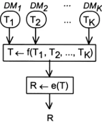
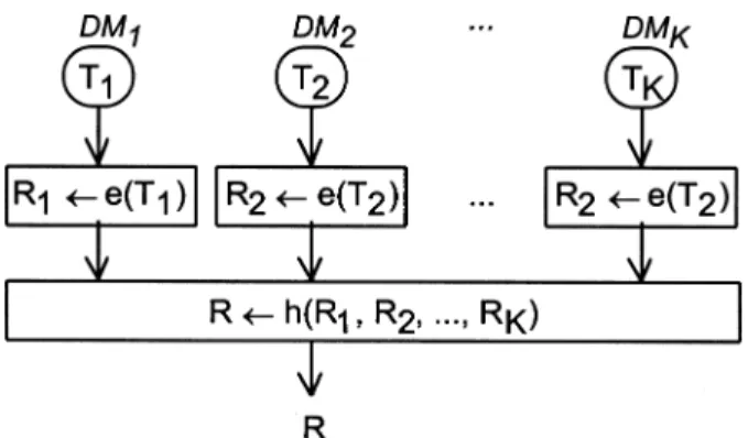
In this framework, group decision processes may be divided according to the level where the individual perspectives are aggregated: either at the input level or at the output level. When aggregation occurs at the input level (Figure 1), an operator f(.) aggregates the individual T_k (k = 1,...,K) into a set T of values accepted by the group, whereas an operator e(.) yields all the results of the method (ELECTRE TRI in our case) compatible with T. When aggregation occurs at the output level (Figure 2), the operator e(.) yields the set of results of the method compatible with each DM’s T_k, whereas an operator h(.) aggregates the individual sets of results R_k into a set of results R. The aggregation performed by f(.) and h(.) may consist in averaging, minimizing a distance measure, voting, etc. For instance, in the context of additive value functions, Kim and Ahn (1997) suggest an approach where h(.) (see Figure 2) is a difference of weighted sums for each pair of actions.

When seeking consensus on what to recommend, it may be appropriate to consider f(.) or h(.) as the set operations ∩ (intersection) or ∪ (union). When using intersections, set R will gather the DMs consensus on the results that should be considered, whereas if the union operation is used, the DMs will agree on the results that should not be considered (those not in R). The remaining of this paper presents a method to obtain all the results

compatible with a set of constraints, i.e. an operator e(.), for the case of the ELECTRE TRI. This operator may be useful in two different types of approach, as follows.

If the aggregation occurs at the input level (Figure 1), f(.) may build T as an intersection of the individual polytopes T₁, ..., T_K of acceptable values for the parameters. In this case, for each action to be assigned, the procedure e(.) will yield a single category or a range of categories compatible with the parameter values that are accepted by all of the group’s members. It may happen that T becomes void, although this should not happen frequently if there is no strong conflict among the DMs. In such cases, the individual polytopes may be changed either by discussing the constraints or by automatically dropping or loosening constraints in a “fair” manner. For instance, a linear program may be solved to find a polytope minimizing some “fair” measure of the violations as regards the original constraints. The approach in the next paragraph may also be used.

A second type of approach performs the aggregation at the output level (Figure 2). In this case, the operator e(.) may be helpful to yield a single category or a range of categories for each individual DM, while h(.) builds R as the reunion of all these results. For each action, a possible assignment is considered by the group (is in R) if it is considered by at least one of its members.

We believe that dealing with imprecise information is not only necessary (given the difficulties in providing precise values for the parameters), but also beneficial in a group setting as described here. Rather than forcing each DM to choose and defend a combination of values, we are inviting DMs to progressively and cooperatively form their convictions as they interact with the decision aid method. The DMs may focus on those actions where imprecise information implies more variability in the output, while they can easily agree on the assignments concerning the remaining actions. Indeed, a potential benefit of the approach proposed here is that the DMs may agree on a result although they would not be able to agree on precise values for the input parameters.

3. An overview of ELECTRE TRI

Let A be a set of m actions a₁, ..., a_m characterized according to multiple attributes. ELECTRE TRI (Yu, 1992; see also Mousseau et al., 1999) is a multicriteria decision aid method that evaluates the absolute merits of each action in A. The method assigns each action to one of k pre-specified ordered categories: C1 _{(the worst), ..., C}k _{(the best). Each category C}i _is limited by two reference actions (profiles): bi _{is its upper limit and b}i-1 _{is its lower limit. Let} B denote the set of k+1 profiles b0_{, ..., b}k_{. Each action in A will be assigned by comparing} it with the profiles in B successively.

Consider any ordered pair of actions (a₁, a₂), where either a₁∈ A and a₂∈ B or vice-versa. We will start by recalling how to compute an index measuring the credibility of the statement “a₁ outranks (is at least as good as) a₂” (for details see Roy, 1991; Roy and Bouyssou, 1993).

Let there be n pseudo-criteria. The j-th criterion (j = 1,...,n) is characterized by an importance coefficient k_j, an indifference threshold q_j, a preference threshold p_j and a veto threshold v_j. These thresholds obey v_j ≥ p_j ≥ q_j ≥ 0. For simplicity of notation we assume that thresholds do not depend on the profiles’ performances and do not vary from profile to profile, but this work could be easily extended to drop this assumption. Let g_j(a₁) and g_j(a₂) denote the performance on the j-th criterion of the actions a₁ and a₂, respectively. Let ∆j represent the advantage of a1 over a2 on this criterion:

{

2) , if the j

th _{criterion is to maximised (the more the better)}

∆j = g_j(a₂) – g_j(a 1) , if the j th _{criterion is to maximised}

{

(

)/(

)

k_jc_j(a₁,a₂), where we assume that n j

= 1

k_j = 1 (3.2)

Σ

Σ

For each criterion (j = 1,...,n), the concordance index regarding the hypothesis “a₁ S a₂” is:

A global concordance index is then computed by aggregating the n single-criterion concordance indices aas a weighted sum using the importance coefficients:

This binary valued relation is transformed into a crisp relation through a cut threshold λ: a₁ outranks a₂ (represented as a₁ S a₂) ⇔ σ(a₁,a₂) ≥ λ.

The following relations can then be defined:

a₁ P a₂ (a₁ is preferred to a₂) ⇔ a₁ S a₂ and not a₂ S a₁; a₁ I a₂ (a₁ is different to a₂) ⇔ a₁ S a₂ and not a₂ S a₁; a₁ R a₂ (a₁ is incomparable to a₂)⇔ not a₁ S a₂ and not a₂ S a₁; The ELECTRE TRI method expects that the profiles in B are such that: – for every action a_x in A, bk _{P a}

x (recall that b

k _{is the upper limit of the best category);} – for every action a_x in A, a_x S b0 _{(recall that b}0 _{is the lower limit of the worst category);} – g_j(b1_{) > g}

j(b

i–1_{), j = 1,...,n; i = 1,...,k;} – bk _{P a}k–1 _{P ... P b}0_;

– every action in A may be indifferent to at most one of the reference actions bi _{(i = 0,...,} k–1).

Finally, there are two variants of the ELECTRE TRI to assign each action in A:

Pessimistic ELECTRE TRI: This variant assigns each action a_i to the highest category Cc such that a_i outranks bc–1_{. An algorithm to perform the assignment could be the following} (Yu, 1992): c ← k (best category); WHILE not a_i S bc–1 _DO c ← c – 1

{

(

)/(

)

Finally, the discordance indices and the global concordance index are combined to yield the credibility index for the hypothesis “a₁ S a₂”:

1 – d_j(a₁, a 2) σ(a₁,a₂) = c(a₁,a₂) 1 – c(a₁,a₂) (3.4) j ∈ {1,...,n}: d_j(a₁,a₂) > c(a₁,a₂)

Π

ΕΝD _– WHILE assign a_i to category Cc

Optimistic ELECTRE TRI:This variant assigns each action a_i to the lowest category Cc such that bc _{is preferred to a}

i. An algorithm to perform the assignment could be the following (Yu, 1992): c ← 1 (worst category); WHILE not bc _{P a} i DO c ← c + 1 END _– WHILE assign a_i to category Cc

Suppose that an action a_i is assigned to category Cp _{by pessimistic ELECTRE TRI and} assigned to category Co _{by optimistic ELECTRE TRI. Then, we know that C}p ≤ _Co _(Yu, 1992).

4. Constraints on the parameter values

We consider that there is imprecise information on the values of the parameters k_j, q_j, p_j and v_j (j = 1,...,n), on the cut threshold λ and on the actions’ performances, provided as a set of bounds and linear constraints. These bounds and constraints may be directly provided by the DMs or inferred through a questioning protocol, as in Mousseau (1993).

To characterize the resulting polytope T, we will take into account some reasonable types of constraints that may appear in practice (where some types of parameters may be varied independently of others). For instance, a constraint such as k₁≥ k₂ is reasonable, whereas the constraint k₁ + λ q₁ is not. First of all, the variation of the cut threshold λ should not depend on any other parameter, hence we assume it will appear only on a single constraint:

λ∈[λ_min,λ_max] (4.1)

Indifference and preference thresholds are local to each criterion and inter-criteria comparisons of these thresholds have no meaning. Therefore, we assume that these may be subject to bound constraints only:

and

up_j≥ p_j≥ lp_j, j = 1,...,n (4.3)

plus

v_j≥ p_j≥ q_j, j = 1,...,n (4.4)

For the j-th criterion (j = 1,...,n), DMs may define a polytope G_j of admissible performances both for actions in A and in B. This polytope is defined by linear constraints such as g_j(a_x) ≥ 3g_j(a_y) or g_j(a_x) ≥ g_j(a_y) + 2. We assume these constraints will satisfy the five conditions presented in Section 3. These constraints can be represented as:

(g_j(a₁), g_j(a₂), ..., g_j(a_m), g_j(b0_), j(b 1_{),..., g} j(b k₎₎ ∈_G j⊂R m+k+1 _{(j = 1,...,n) (4.5)} Concerning importance coefficients, we also assume that the DMs define a polytope K through linear constraints, such as k_i≥ α k_j, L_j≥ k_i ≥ I_j, α_a k_a + α

b kb + ... + αc kc≥ 0, or k1 + k₂ + ... +k_n = 1. These constraints can be represented as

k =(k₁,...,k_n) ∈ K ⊂ Rn _(4.6)

Finally let us consider the veto thresholds. Veto thresholds carry information concerning how important each criterion is, relative to others. Hence, the veto threshold value for one criterion may be constrained by veto threshold values for other criteria. We consider three different situations:

Type 1: (bounds only) uv_j ≥ v_j≥ lv_j, j = 1,...,n; (4.7a) Type 2: (polytope) v = (v₁,...,v_n) ∈ V ⊂ Rn_{; (4.7b)} Type 3: (dependence on k_j) v_j = p_j + α_j/k_j, with uα_j≥α_j≥ lα_j, j = 1,...,n.

(4.7c) Constraints such as α_m q_j≤ p_j≤α_M q_j or β_m p_j≤ v_j≤β_M p_j may be useful and could also be accepted. As general assumptions, we require all parameters to be non-negative and G_j (j = 1,...,n), K and V to be compact (closed and bounded), so that T is a polytope. Mousseau (1993) has devised a questioning protocol and a computer program to obtain (4.2), (4.3), (4.6) and (4.7a) from the DMs’ answers.

5. Worst case and best case categories

5.1. First algorithms

Considering any admissible combination of parameters, ELECTRE TRI (pessimistic or optimistic variant) assigns each action to a category. Our aim is to adapt the method to determine which categories the action will be assigned to under the best and worst possible cases. Let B(a_i) and W(a_i) denote he highest and lowest categories, respectively, that action a_i may belong to. The premises “a_i belongs to a category between W(a_i) and B(a_i)”, “a_i does not belong to category worse than W(a_i) and B(a_i) coincide the assignment is robust: new information (tighter constraints) would bring no benefit.

The algorithms by Yu (1992) (see Section 3) may be adapted to determine B(a_i) and W(a_i), for a given a_i∈A. Consider the region T of admissible values for the parameters and t∈T. Let a₁ S(t) a₂ denote an outranking of action a₁ over action a₂ when parameters take values t; a₁ P(t) a₂ denote a₁ S(t) a₂¬Ø[a₂ S(t) a₁] (where ¬ is the negation operator).

The adapted algorithms will use the following proposition (these results are easy to prove, see Roy and Bouyssou, 1993, pp. 92–93):

Proposition 5.1. Let a_i∈ A and let bc _{be a reference action. Then,} a_i S(t) bc⇒ _a i S(t) b c–1 _{and a} i P(t) b c⇒ _a i P(t) b c–1 _{(c = 1, ..., k);} ¬(a_i S(t) bc₎ ⇒ ¬_(a i S(t) b c+1_{) and} ¬_(a i P(t) b c⇒ ¬_(a i P(t) b c+1_{) (c =} 0, ..., k-1).

Considering Prop. 5.1, the following algorithms are valid: Pessimistic ELECTRE TRI:

To find worst case category W(a_i) To find best case category B(a_i): c ← k;/*best category*/ c ← k;/*best category*/

WHILE ∃t∈ T: ¬_(a i S(t) b c–1_{) DO WHILE t}∈ _T, ¬_(a i S(t) b c–1_{) DO} c ← c – 1 c ← c – 1 END_WHILE END_WHILE W_p(a_i) ← Cc_{. B} p(ai) ← C c_.

Optimistic ELECTRE TRI:

To find worst case category W(a_i): To find best case category B(a_i):

c ←1;/*worst category*/ c ← 1;/*worst category*/ WHILE t∈ T, ¬_(bc _{P(t) a} i) DO WHILE t∈ T: ¬_(bc _{P(t) a} i) DO c ← c + 1 c ← c + 1 END_WHILE END_WHILE A A

W_o(a_i) ← Cc_{. B} o(ai) ← C

c_.

These algorithms show that absolute robust conclusions pertaining to the category where an action a_i is assigned are equivalent to a conjunction of several relative binary robust conclusions concerning the outranking relation among a_i and some of the reference actions.

5.2 Equivalent faster algorithms

We shall see in Section 6 that the test performed at each iteration of the algorithm may not be straightforward to compute. Hence, it may be useful to improve the algorithms presented above, especially if there are more than just a few categories. First of all, note that the pessimistic TRI algorithms search for the assignment category starting from the best one (Ck_{), whereas optimistic TRI algorithms’ search starts from the worst category (C}1_{). Since} we know that the pessimistic search will stop at a category lower or equal than the one where the optimistic search stops, modified algorithms could be used instead. A new version of the algorithms could start the search in the opposite direction from those of Section 5.1. These searches have complexity O(k) (where k is the number of categories).

A binary search of complexity O(log k) is even better, particularly if the number of categories is high. Given an interval of categories, we test whether a_i belongs to a category above or below the middle of the interval considered. Based on this test, half of the interval is ignored and the other half is bisected in the next iteration. In order to present a more general algorithm, let test(t) be a Boolean function that changes according to the purpose of the computation:

t ∈ T, a_i S(t) bc _{to find W}

p(ai) in the pessimistic ELECTRE TRI ∃ t ∈ T: a_i S(t) bc _{to find B}

p(ai) in the pessimistic ELECTRE TRI t ∈ T, ¬(bc _{P(t) a}

i) to find Wo(ai) in the optimistic ELECTRE TRI ∃ t ∈ T: ¬(bc _{P(t) a}

i) to find Bo(ai) in the optimistic ELECTRE TRI Then, a new algorithm can be written as follows:

ELECTRE TRI (Binary Search Version) L ← lower _– bound

U ← upper _– bound WHILE L <U DO

c ← (L + U)/2;/∗x: max {n ∈ N: n ≤ x}*/ If test(t) returns true THEN L ← c + 1 ELSE U ← c; END_–WHILE

result category is CL_{./*result is W}

p(ai), Bp(ai), Wo(ai) or Βο(aι) depending on test(t)*/

A A

Note that we may start with a tighter search interval whenever some related problems have already been solved, because we know that W_p(a_i) ≤ B_p(a_i), W_o(a_i) ≤ B_o(a_i), W_p(a_i) ≤ W_o(a_i) and B_p(a_i) ≤ B_o(a_i). Therefore, lower_bound ←1, or higher if more information is available from a previously determined result, whereas upper_bound ←k, or lower if more information is available.

6. On determining the results of the tests

6.1. Formulation as optimization problems

In Section 5.2 we presented several forms for test(t). In this section we show how optimization may be used to determine if the test returns true or false. To simplify notation, we omit t in σ(.,.,t), but bear in mind that the credibility index depends on the parameter values.

To find B_p(a_i) in the pessimistic TRI:

∃ t ∈ T,: a_i S(t) bc⇔ _max{σ_(a i,b

c_{): t} ∈ _T} ≥ λ min.

Note that, since an iterative algorithm will be used to solve this maximization problem, it may find that the test is true before reaching the optimum.

To find B_o(a_i) in the optimistic TRI:

∃ t ∈ T: ¬(bc _{P(t) a}

i) ⇔∃ t ∈ T:

¬_(bc _{S(t) a}

i) ∨ ai S(t) b c

The formulation as optimization problems is the following: ∃ t ∈ T: ¬(bc _{P(t) a} i) ⇔ min{σ(b c_,a i): t ∈ T} < λmax∨ max{σ(ai,b c_{): t} ∈ _T} ≥ λ min

The two optimization problems may be performed in arbitrary order, and the second problem only needs to be solved if the first one yields false.

To find W_p(a_i) in the pessimistic TRI:

A

t ∈ T, a_i S(t) bc⇔ _min{σ_(a i,b

c_{): t} ∈ _T} ≥λmax_;

Note that an iterative algorithm to solve this minimization problem may find that the test is false before reaching the optimum.

To find W_o(a_i) in the optimistic TRI: t ∈ T, ¬(bc _{P(t) a} i) ⇔ t ∈ T, ¬_(bc _{S(t) a} i) ∨ ai S(t) b c

is true if and only if the system t ∈ T (which includes bounds on λ) σ(bc_,a

i)-λ≥ 0 σ(a_i,bc_)-λ _{< 0}

is inconsistent. This can also be formulated as an optimization problem, for instance: t ∈ T, ¬(bc _{P(t) a}

i) ⇔ min{σ(ai,b

c_)-λ_{: t} ∈ _T ∧σ_(bc_,a

i)-λ≥ 0} ≥ 0.

We will see that this optimization problem is hard to solve for constraints of type 2 or 3 (recall Section 4). However, we may avoid performing these tests at every iteration, based on the following:

Proposition 6.1.:

Let C° denote the category where action a_i is assigned to by the optimistic TRI and let Cm denote min{Cj _(j ∈_{{1,...,k}): b}j _{S a}

i}.

Then, either C° = Cm _{or C° = C}m+1_{. Furthermore, if C° = C}m+1 _{then b}m _{I a} i. Proof: We defined Cm _{to be the lowest category such that b}m _{S a}

i. If

¬_(a

i S b

m_{), then b}m _{P a} i, which means that C° = min{Cj _(j ∈ _{{1,...,k}): b}j _{P a}

i} = C m_. Otherwise, if a_i S bm_{, then b}m _{I a}

i, and C° > C

m_{. Consider now the category C}m+1_{. Since} bm _{S a}

i, then b m+1 _{S a}

i. On the other hand, ai may not be indifferent to more than one category (Yu, 1992). Since bm _{I a}

i, we conclude that

¬_(bm+1 _{I a}

i), hence we must have b m+1 _P a_i. In that case, C° = min{Ci _(i∈_{{1,...,k}): b}i _{P a}

i} = C m+1_. To find Cm _{= min{C}i _(i∈_{{1,...,k}): b}i _{S a}

i}, test(t), which is performed many times, becomes: t ∈ T, ¬_(bc _{S(t) a}

i) ⇔ max{σ(b c_,a

i): t ∈ T} < λmin.

Note that an iterative algorithm to solve this problem may find that the test is false before reaching the optimum. Then, only a test will remain to be performed:

∃t∈T: bm _{P(t) a} i⇔ min{σ(ai,b m_)-λ_{: t} ∈ _T ∧σ_(bm_,a i)-λ ≥ 0} < 0. A A A A

If true, then a_i belongs to Cm_{; if false, a}

i belongs to C

m+1_{. Note that this test is performed} only once. An iterative algorithm may find that the test returns true before reaching the optimum.

6.2. On finding the best category for an action

We now discuss the problem of finding the best category that an action a_i may attain subject to t ∈ T. Consider, without loss of generality, that the binary search algorithm of Section 5.2 is being used. If the pessimistic TRI is chosen, we must solve at each loop iteration the optimization problem max{σ(a_i,bc_{): t} ∈ _{T} until we get a solution with value} higher or equal to λ_min or we reach the maximum. If the optimistic TRI is chosen, we can start by solving in each iteration the problem max{σ(a_i,bc_{): t} ∈ _{T}, until we reach a solution} with value higher or equal to λ_min or we reach the maximum. If we reach a minimum value lower than λ_min, then we must solve min{σ(bc_,a

i): t ∈ T} until we reach a solution with value lower than λ_max or we reach the minimum.

Next we address the problems max{σ(a_i,bc_{): t} ∈ _{T} and min{}σ_(bc_,a

i): t ∈ T} separately. Let ∆_j represent the advantage of a_i over bc _{on the j-th criterion (j = 1, ..., n). Let J}C _denote the set j ∈ {1,...,n: ∆_j≥0}, JD _{denote the set j}∈_{1,...,n: ∆

j<0}, and J

V _{denote the set j} ∈_{1,...,n: ∆j < -pj} (after F∅ and F1 below have been performed).

To solve max{σσσσσ(a_i,bc_{): t} ∈∈∈∈∈ _T}:

In recalling the definition of the polytope T (Section 4), note that only some of the parameters are interdependent. Concerning the jth _{criterion, the performances g}

j(ai), gj(b

c_{) (j = 1,...,n)} are only constrained to belong to G_j, hence we may separately find which combinations of performances are most favorable to a_i, through n linear programs (P∅ below). Parameters p₁, ..., p_n, q₁, ..., q_n are only subject to lower and upper bounds. Hence, we may fix them (F∅ below) to the values that most benefit a_i and least benefit bc _{(see appendix, Prop. A.1).} Bounds should satisfy constraints v_j≥ p_j≥ q_j (j = 1,...,n). The optimization of the values for other parameters depends on the type of the constraints affecting the veto thresholds (4.7a-c).

Type 1 (veto subject to bounds)

P∅∅∅∅∅:solve max{∆_j: (g_j(a₁), ...,g_j(a_m), g_j(b0_{), ...,g} j(b k₎₎ ∈_G j}, j = 1,...n. F∅: q_j← uq_j; p_j← up_j, j∈JD _{and q} j← lqj; pj← lpj j∈J C_. F1: v_j← uv_j, j∈JD _{and v} j← lvj , j∈J

C_{. (Fixed according to appendix, Prop. A.1)}

PM1: solve max{c(a_i,bc_{, k): (k}

1,...,kn) ∈K. (Linear program, see appendix, Prop. A.2). max s(a_i,bc_{) is now immediately obtained by combining the results of these steps.} Type 2 (veto subject to linear constraints, but independent of importance coefficients)

P∅∅∅∅∅, F∅: (same as above)

PM1:(same as above)

If the optimal value c(a_i,bc_{)* is 1, then max} σ_(a i,b

c_{) is 1; else consider c(a} i,b

c_{)*, add} constraints to guarantee that no veto occurs and continue (note that these constraints are linear and σ(a_i,bc_{)=0 when they are violated):}

PM2: solve max σ(a_i,bc_{,v): (v}

1,...,vn) ∈V, vj≥-∆j + ε (j∈J

V_{)}, where} ε _{is a small positive} number (if there is no feasible solution then max σ(a_i,bc_{) is 0).}

Type 3 (veto is a function of the importance coefficient)

P∅∅∅∅∅, F∅: (same as above) F3: α_j ← uα_j, j∈JD _and α j← lαj, j∈J C_{. (Most favorable to a} i, least favorable to b c₎ PM3: solve max σ(a_i,bc_{, k): (k} 1,...,kn)∈K, kj ≤αj/[-∆j - pj] -ε (j∈J V_)},

where ε is a small positive number (if there is no feasible solution then max σ(a_i,bc_{) is 0).}

To solve min{σσσσσ(bc_,a

i): t∈∈∈∈∈T}. Much of the process is similar to that of solving max{σ(ai,b c_): t∈T, hence we only highlight the differences.

Type 1 (veto subject to bounds)

P∅∅∅∅∅, F∅, F1:(same as above)

Pm1: solve min {c(bc_,a

i,k): (k1,...,kn)∈K}. (Yielding min σ(b c_,a

i))

Type 2 (veto subject to linear constraints, but independent of importance coefficients)

P∅∅∅∅∅, F∅: (same as above) If ∃(v₁, ..., v_n) ∈V, j∈JC_{: v}

j≤ ∆j (veto occurs) then min σ(b c_,a

i) = 0; else:

Pm1: (same as above) If the optimal value c(bc_,a

i)* is 0, then min σ(b c_,a i) is 0; else consider c(b c_,a i)* and continue: Pm2: solve min σ(bc_,a i,v): (v1,...,vn)∈V}.

Type 3 (veto is a function of the importance coefficient)

P∅∅∅∅∅, F∅, F3:(same as above) If ∃ (k₁, ..., k_n)∈K, j∈JC_{: k}

j≥ αj/[∆j – pj] (veto occurs) then min σ(b c_,a

i) = 0; else:

Pm3: solve min {σ(bc_,a

i,k): (k1,...,kn)∈K}. 6.3. On finding the worst category for an action

We discuss in this section the problem of finding the worst category that an action a_i may attain subject to t∈T. Consider again that the binary search algorithm of Section 5.2 is being used. If the pessimistic TRI is chosen, we must solve at each loop iteration the optimization problem min{σ(a_i,bc_{): t}∈_{T} until we get a solution with value lower} than λ_max or we reach the minimum. If the optimistic TRI is chosen, according to Prop. 6.1, we can solve at each iteration the problem max{σ(bc_,a

i): t∈T} until we reach a solution with value higher or equal to λ_min or we reach the maximum. The algorithm will then stop with the output category Cm_=min{Cj _(j∈_{{1,...,k}): b}j _{S a}

i}. Afterwards, we need to solve {min σ(a_i,bm_)-λ_{: t}∈_T ∧ σ_(bm_,a

i)-λ ≥ 0} once. Next we address all these problems separately.

To solve min {σ{σ{σ{σ{σ(a_i,bc_{): t}∈∈∈∈∈_{T}: See Section 6.2. The problem is analogous to min} σ_(bc_,a i): t∈T}, with bc _{and a}

i interchanged.

To solve max{σσσσσ(bc_,a

i):t∈∈∈∈∈T}: See Section 6.2. The problem is analogous to max{σ(bc_,a

i):t∈T}, with b c _{and a}

To solve min{σσσσσ(a_i,bm_)-λλλλλ_{: t}∈∈∈∈∈_T ∧∧∧∧∧σσσσσ_(bm_,a

i)-λλλλλ≥≥≥≥≥ 0}. The process is similar to min{σ(ai,b c₎ (with bm _{in place of b}c_{) with an additional constraint. Let} ∆

j, J

C _{and J}D _{(as defined in} Section 6.2)

now refer to bm _{instead of b}c_. Type 1 (veto subject to bounds)

Pa∅∅∅∅∅: solve min{∆_j: (g_j(a₁), ...,g_j(a_m), g_j(b0_{), ...,g} j(b k₎₎∈_G j}, j = 1,...n. Fa∅: q_j← lq_j; p_j← lp_j, j∈JD _{and q} j← uqj; pj← upj, j ∈J C_. Fa1: v_j← lv_j, j∈JD _{and v} j← uvj, j∈J C_.

Pa1: solve min{c(a_i,bm_,k)-λ_{: (k}

1,...,kn)∈K, λ∈[λmin,λmax], σ(b m_,a

i,k)-λ ≥ 0}.

Type 2 (veto subject to linear constraints, but independent of importance coefficients)

Pa∅∅∅∅∅, Fa∅: (same as above)

Pa2: solve min{σ(a_i,bm_,k,v)-λ_{: k}∈_{K, v}∈_V, λ∈_[λ

min,λmax], σ(b m_,a

i,k,v)-λ≥ 0}. Type 3 (veto is a function of the importance coefficient)

Pa∅∅∅∅∅, Fa∅: (same as above)

Pa3: solve min{σ(a_i,bm_,k)-λ_{: (k}

1,...,kn)∈K, λ∈ [λmin,λmax], σ(b m_,a

i,k)-λ ≥ 0}. 6.4. Solving the subproblems

Among the (sub)problems presented in Sections 6.2 and 6.3, problems P∅, PM1, Pm1 and Pa∅ are linear in the objective function and in the constraints, hence they may be solved by any linear programming algorithm. The remaining problems are generally more difficult to solve since they are nonlinear in the objective function and sometimes also nonlinear in the constraints (the case of Pa1, Pa2 and Pa3).

The functions to maximize in problems PM2 and PM3 are strictly quasiconcave (see Appendix, Prop. A.4 and A.7). Therefore, any local maximum of these nonlinear programs must be a global maximum (e.g. see Bazaraa et al. (1993)). Another approach for PM2 is to maximize the logarithm of σ(.), as a separable concave function (see Prop. A.5 in appendix). The search for the maximum is simplified, because the constraints are linear. However, this search must account for the nondifferentiability of the objective function. In Lemaréchal (1989) and references contained therein the reader may find many methods to cope with nonsmooth problems like these, that use generalized notions of derivatives and gradients. Most of these consider the problem of minimizing a convex function, or, equivalently, maximizing a concave function, that fortunately may often be extended to address quasiconcavity (e.g. see Gromicho, 1998)).

The same functions are to be minimized in problems Pm2 and Pm3. These are global optimization problems, which are difficult as there may exist multiple local minima. However, since the objective functions are strictly quasiconcave and the constraints define a polytope, then the global minimum of each one of these nonlinear programs can be found at an extreme point of the polytope (e.g. see Bazaraa et al. (1993), p. 107, for a proof). Horst and Tuy (1996) present several efficient methods to deal with such quasiconcave minimization problems. Moreover, if the polytopes K and V do not have many vertices, and considering that they will be used repeatedly for many problems with

different pairs of actions (where only the objective function changes), then an algorithm for enumerating all their vertices (e.g. Avis and Fukuda, 1992) may be run once, and then the list of vertices can be searched as needed.

Problems Pa1, Pa2 and Pa3 can be more difficult since there is an additional nonlinear constraint. Fortunately, they are only needed when determining the worst case for the optimistic TRI and are solved only once per action to sort. A property shared by these problems, which can be exploited, is that the credibility function is strictly quasiconcave (propositions A.3, A.6 and A.7). Hence, it attains its minimum at an extreme point of the feasible region, which is convex. The global minimum is located either at a vertex of the polytope defined by the linear constraints (note that some vertices may now be unfeasible) or at the surface where σ(bm_,a

i,.)=λ. In the case of problem Pa2, the independence among the constraints on importance coefficients and those on veto thresholds might also be exploited. Methods to deal with this sort of concave minimization problems can be found in Horst and Tuy (1996). For a more general review of global minimization see Rinnooy Kan and Timmer (1989).

It is important to notice two aspects that can significantly decrease the computational burden associated with all the problems of Sections 6.2 and 6.3. First, note that often one may find whether a test is true or false before reaching the optimum (recall Section 6.1). To benefit form this, we should use feasible-iteration optimization algorithms, i.e. algorithms producing a sequence of feasible solutions converging to the optimum, instead of approaches based on exterior approximations to the feasible region. Secondly, when using these iterative optimization algorithms, we may start at the feasible solution where we stopped at an earlier problem. For instance, suppose we were solving the problem max{σ(a_i,bx_{): t}∈_T}, until we stopped at solution with value higher or equal to λ_min or at the maximum (whatever occurred first). Then, when solving a problem max{σ(a_i,by_{): t}∈_{T}, with x}≠_{y, we would} start iterating at the point where we had left the prior problem, instead of starting from some other initial (possibly unfeasible) solution.

7. Illustrative example

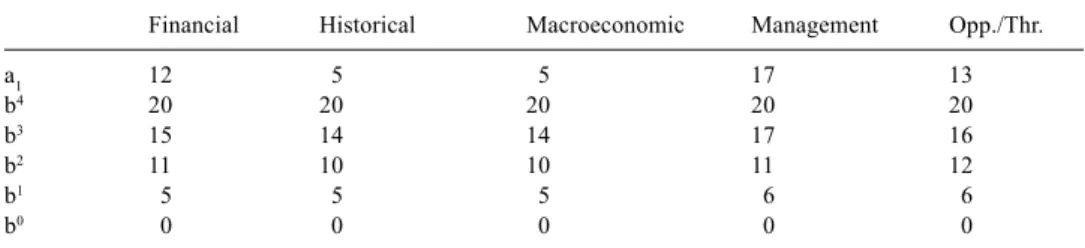
As a small example, let us consider that the DMs’ purpose is to assign each action (corresponding to a company) to a risk category (“bad”-C1_{, “neutral”-C}2_{, “good”-C}3_{, “very} good”-C4_{), according to five criteria: a financial dimension (assets, liabilities, etc.), an} Table 1. Performances of the action to be assigned and the reference actions (profiles)

Financial Historical Macroeconomic Management Opp./Thr.

a₁ 12 5 5 17 13 b4 _{20 20 20 20 20} b3 _{15 14 14 17 16} b2 _{11 10 10 11 12} b1 _{5 5 5 6 6} b0 _{0 0 0 0 0}

historical dimension (credit incidents, reputation, etc.), a macroeconomic dimension (region, sector of activity, etc.), a management dimension (qualification, commitment, etc.), and an opportunities and threats dimension (competitors, evolution of the market, etc.). Suppose all of these have been quantified on a 0–20 rating scale. We consider the assignment of an action a₁ whose performances are depicted in Table 1, together with the performances of the reference actions.

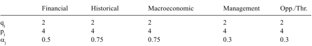
In this example we consider fixed performances and fixed indifference and preference thresholds (Table 2). The veto threshold is a function of the importance coefficients, v_j = p_j + αj/k_j, and the fixed parameters αj in Table 2. Finally, let the cut threshold λ = 2/3. The imprecise information concerns the importance coefficients k_j and, since v_j = p_j + αj/k_j, it also affects the value of the veto coefficients v_j (Type 3 constraints). Suppose that the information by the DMs leads to the following constraints:

k₂≥ k₃ k₂≤ 2 k₃ k₁≥ k₂ k₁≤ k₂ + k₃

k₅≥ k₁ k₅≥ 2 k₂ k₅≤ 2 k₂ + k₃ k₄≥ k₅ k₄≥ k₁ + k₂ +k₃ k₄≤ k₁ + k₂ + k₃ + k₅

To assign a₁ by the pessimistic TRI using the binary search algorithm we could start by finding the best possible category for a₁. First, we would compare it to b2 _{to find if} max{σ(a₁,b2_):t∈_{T} exceeds} λ _{= 2/3. Using Excel’s Solver for nonlinear programming} resolves this problem, although this solver expects differentiable functions. In 5 iterations (instantaneous time) it tells us that the maximum is 0.864 > λ, hence a₁ belongs to category C3 _{or higher. Then, a}

1 would be set against b

3 _{to find if max{}σ_(a 1,b

3_{): t}∈_{T} exceeds} λ _{= 2/3.} We would find that the solution has a value of 0.682 >λ, hence a₁ may reach category C4_.

To find the worst pessimistic assignment for a₁ we would first compare it with b2 _{to find} how min{σ(a₁,b2_{): t}∈_{T} compares to} λ _{= 2/3. Using the method by Avis and Fukuda (1992)} to enumerate all the 16 vertices of this polytope, we calculate σ(a₁,b2_{) at each vertex solution} and find a minimum value of 0.75 > λ. Hence, hence a₁ belongs to category C3 _{or higher.} Next we compare it with b3 _{and find that min{}σ_(a

1,b

3_{): t}∈_{T}= 0.063<} λ _{(at a different} vertex solution). Hence a₁ now belongs to category C3_{. In conclusion, under these constraints} it is possible to conclude that the range of categories that a₁ may belong to is {“good”, “very good”}.

Table 2. Information on thresholds

Financial Historical Macroeconomic Management Opp./Thr.

q_j 2 2 2 2 2

p_j 4 4 4 4 4

Suppose now that we replaced the last constraint k₄ ≤ k₁ + k₂ + k₃ + k₅ by a tighter constraint k₄≤ k₁ + k₅ and repeated the process. To find the best category we would see that max{σ(a₁,b2_):t∈_{T} is 0.842 >} λ _{(5 iterations) and then would find that max{}σ_(a

1,b 3_): t ∈T} is 0.628 < λ (14 iterations more, but still instantaneous). Hence, the best category attained by a₁ is now C3_.

Concerning the worst category, we would find that min{σ(a₁,b2_{): t}∈_{T} would remain} the same, as would min{σ(a₁,b3_{): t}∈_{T}. In conclusion, after tightening the last constraint it} is possible to conclude that the a₁ belongs to category “good”. Although there is imprecise information, it was possible to determine a precise assignment for this action.

action.

In a group decision-making framework, a method to find the best and worst categories that each action may attain may be used in a conjunctive or disjunctive manner. The former consists in accepting an assignment as possible if the input of all of the DMs warrants that conclusion. The latter consists in accepting an assignment as possible if any DM, individually, reaches that conclusion. A potential benefit arising from this approach is that DMs may agree on a result although they would not be able to agree on precise values for the input parameters.

We have shown how to find the best and worst categories that an action may belong to given linear constraints on the parameter values. To achieve this we changed the tests in the original algorithms. Since these tests involve solving some mathematical programs, we presented versions of these algorithms that are more efficient when there are many categories. We then focused on these tests and suggested some ways to solve these mathematical programs, considering a reasonable set of constraints where some parameters may vary independently from others. A small example was provided to illustrate the feasibility of this approach.

In addition to its potential to discover robust conclusions and to facilitate consensus reaching in group decisions, this approach allows to identify which results are more affected by the fact that information is imprecise. Indeed, it may be interesting to know that some actions have a wide range of categories where they may be assigned to, in contrast with some other actions that are always assigned to a single category. This ranges may in turn be used to prompt discussions about the parameter values, leading to the incorporation of new information in an interactive way.

In Dias and Clímaco (1999) we present some further examples of credibility indices’ maximization and minimization, which show that despite difficult in theoretical terms, the nonlinear optimization problems may be easily solved in practical situations.

8. Summary and future research

ELECTRE TRI is a well-known multicriteria method to assign actions to ordered predefined categories. We addressed the use of this method by a group of DMs with imprecise information on the values of its parameters. This approach potentially eases the burden of each DM, in that precise values for the parameters are no longer required. Moreover, in a group setting it also may help DMs to reach a consensus on what to recommend for each

Future research may address the choice of the best algorithms to solve the optimization problems. As in other circumstances (e.g. Dias et al., 1997), parallel processing may play a positive role. Another stream of research is how to help the DMs in reaching a consensus on set T of acceptable values for the parameters. Regarding this stream, research is needed to guide the DMs in “narrowing” the set T as consensus emerges or more information becomes available.

Acknowledgements

We have used David Avis’ LRS software, available at the ftp site mutt.cs.mcgill.ca (directory pub/C). This research has been partially supported by Technological Development and Scientific Research contract PRAXIS/PCSH/C/CEG/28/96.

Appendix

This appendix presents some results concerning the credibility index function σ(a₁,a₂, t), where t is a combination of parameter values in a given polytope T. For more detail and proofs not presented here see Dias and Clímaco (1999). We will assume throughout that the computation concerns the ordered pair (a₁,a₂), hence we will sometimes refer to the credibility function as σ(t): T → [0,1]. Let ∆_j denote the advantage of a₁over a₂ on the j-th criterion (j = 1, ..., n).

The function

is obviously continuous but it has no derivative in a discrete number of points of T, since neither c(.) nor d_j(.) have. Function σ(t) is a monotonous function of c(t). Furthermore, it increases when any c_j(t) increases and/or any d_j(t) decreases. The following proposition shows how σ(t) changes when some parameters vary.

Proposition A.1.: If any ∆_j , q_j , p_j or v_j increases (j∈{1,...,n}), then σ(a₁,a₂) does not decrease. Now consider the constraint (k₁,...,k_n) = k∈K (4.6). The next proposition states that the global concordance index c(k) = c(a₁,a₂, k):K → [0,1] is linear on k:

Proposition A.2.: Given fixed values for q_j, p_j and ∆_j (j = 1,...,n), x, y∈K, λ∈ [0,1], c((1-λ) x+λy) = (1-λ) c(x) + λ c(y).

Proposition A.3.: Given fixed values for q_j, p_j, ∆_j and v_j (j = 1,...,n), σ(k) is both strictly quasiconvex and strictly quasiconcave, i.e.

1–dj (a1, a2,t) σ (t) = σ(a₁, a₂,t) = c(a₁,a₂,t)

Π

A

λ∈]0,1[,x,y∈K, σ(x) ≠σ(y) ⇒ max{σ(x), σ(y)} > σ((1-λ)x + λy) > min{σ(x), σ(y)}. Proof: This is a corollary of Prop. A.2 together with the fact that σ(t) is a monotonous function of c(t). Let for instance σ(x) > σ(y). Then, by monotony, c(x) > c(y). Hence:

c(x) > c((1-λ)x + λy) = (1-λ) c(x) + λ c(y) > c(y), and again by monotony σ(x) > σ((1-λ)x + λy) > σ(y).

Next we consider the cases when veto thresholds cannot vary independently, i.e. constraints of type 2 and type 3.

Type 2 constraint

First let us consider a constraint (v₁,...,v_n) = v∈V (Type 2). We assume that q_j, p_j, ∆_j and k_j (j = 1,...,n) are fixed, that c(a₁,a₂, k) < 1 (else we know that the credibility index equals one) and that no veto occurs (i.e. v_j ≥ -∆_j, j = 1,...n). The following proposition establishes that σ(v) is strictly quasiconcave in a subset U⊆V. Note that σ(v) is null for v outside of U. Proposition A.4.:Let U = {v∈Rn_{: v}

j≥-∆j (j = 1,...,n)}. Then σ(v) is strictly quasiconcave in U, i.e. λ∈]0,1[,x,y∈U, σ(x) ≠σ(y) ⇒ σ((1-λ)x + λy) > min{σ( x), σ(y)}

Another interesting property of σ(v) is the following, which states that if we wish to obtain a separable function by taking logarithms we keep the concavity property.

Proposition A.5.: ln σ(v) is concave in U = {v∈Rn_{: v}

j > -∆j (j = 1,...,n).

Now suppose we drop the assumption that the k_j (j = 1,...,n) are fixed. Let the constraints on the importance coefficients be independent form the constraints on the veto thresholds, i.e. σ(k,v):KxV→[0,1]. Then σ( k,v) is strictly quasiconcave in the region where veto does not occur:

Proposition A.6.: Let U = {v∈Rn_{: v}

j≥-∆j (j = 1,...,n)}. Then σ(k,v) is strictly quasiconcave in KxU, i.e. λ∈]0,1[, (ka_,va_{), (k}b_,vb₎∈_KxU,

σ(ka_,va₎ ≠σ_(kb_,vb₎ ⇒σ_((1-λ_{) (k}a_,va_{) +} λ _(kb_,vb_{)) > min{}σ_(ka_,va_), σ_(kb_,vb_)}. Proof: Note that when c(k) < 1 (if c(k) =1 then σ(k) = 1) we can write (2.4) as:

A A A

where m_j (k,v_j) = min {1 – c(k), 1 – d_j(v_j)}. Now note that c(k) is linear (Prop. A.1) and, in the

Since m_j (k,v_j) = min {1 – c(k), 1 – d_j(v_j)} is the minimum of a linear function and a concave function, it is concave. Then, to see that σ(k,v) is strictly quasiconcave in KxU follow the proof in Dias and Clímaco (1999) for quasiconcavity in the case of type 3 constraints.

Type 3 constraint

We can prove a result similar to Prop. A.4 for the case with constraints (k₁,...,k_n) = k∈K, v_j = p_j+α_j/k_j and uα_j≥α_j ≥ lα_j (j = 1,...,n) (Type 3). We assume that q_j, p_j, ∆_j and α_j(j = 1,...,n) are fixed, and 0<σ( x)<σ(y)<1:

Proposition A.7: Let I={x∈K: σ(x)∈]0,1]. Then σ(x) is strictly quasiconcave in I, i.e.

λ∈]0,1[,x,y∈I, with σ(x) ≠σ(y), σ((1-λ)x + λy) > min{σ(x), σ(y)}

References

Athanassopoulos, A. D., and V. V. Podinovski. (1997). “Dominance and Potential Optimality in MCDA with Imprecise Information,” Journal of the Operational Research Society 48, 142–150.

Avis, D., and K. Fukuda. (1992). “A Pivoting Algorithm for Convex Hulls and Vertex Enumeration of Arrangements and Polyhedra,” Discrete and Computational Geometry 8, 295–313.

Bana e Costa, C. A., and Ph. Vincke. (1995). “Measuring Credibility of Compensatory Preference Statements When Trade-Offs are Interval Determined,” Theory and Decision 39, 127–155.

Bazaraa, M. S., H. D. Sherali, and C. M. Shetty. (1993). Nonlinear programming: theory and algorithms, 2nd Ed., Wiley.

Dias, L., J. P. Costa, and J. N. Clímaco. (1997). “Conflicting Criteria, Cooperating Processors – Some Experiments on Implementing a Multicriteria Decision Support Method on a Parallel Computer,” Computers and Operations Research 24, 805–817.

Dias, L.C., and J. N. Clímaco. (1999). “On Computing ELECTRE’s Credibility Indices Under Partial Information,” Journal of Multi-Criteria Decision Analysis 8, 74–92.

French, S. (1995). “Uncertainty and Imprecision: Modelling and Analysis,” Journal of the Operational Research Society 46, 70–79. 1–d_j (v_j) c(k) n σ (k,v) = c (k) Π = Π m_j(k,v_j), 1–c(k) (1–c(k)n _{j = 1} j ∈{1,...,n} d_j(v_j) > c(k) 0 ,if ∆_j ≥ p_j absence of veto, d_j(v_j) = – ∆_j – p_j ,if ∆_j < - p_j, vj – pj

which is either constant if p_j≥−∆_j) or convex.

{

Gromicho, J. (1998). Quasiconvex optimization and location theory, Applied Optimization 9, Kluwer, Dordrecht. Hazen, G. B. (1986). “Partial Information, Dominance and Potential Optimality in Multiattribute Utility Theory,”

Operations Research 34(2), 297–310.

Henggeler Antunes, C., and J. N. Clímaco. (1992). “Sensitivity Analysis in MCDM Using the Weight Space,”

Operations Research Letters 12, 187–196.

Horst, R., and H. Tuy. (1996). Global optimization: deterministic approaches, 3rd Ed., Springer.

Kim, S.-H., and B.-S. Ahn. (1997). “Group Decision Making Procedure Considering Preference Strength Under Incomplete Information,” Computers and Operations Research 24, 1101–1112.

Lemaréchal, C. (1989). “Nondifferentiable optimization,” in G. L. Nemhauser et al. (eds.) Handbooks in Operations Research/Management Science, Vol. 1. Elsevier, 529–572.

Mousseau, V. (1993). Problémes liés à l’evaluation de l’importance relative des critères en aide multicritère à la décision: refléxions théoriques, experimentation et implémentation informatique, PhD Thesis, Université Paris-Dauphine.

Mousseau, V., R. Slowinski, and P. Zielniewicz. (1999). ELECTRE TRI 2.0a: Methodological Guide and User’s Manual, Document du LAMSADE, No. 111, Université Paris-Dauphine.

Raiffa, H. (1982). The art and Science of Negotiation. Harvard University Press, Cambridge (Ma).

Rinnooy Kan, A. H. G., and G. T. Timmer. (1989). “Global optimization,” in G. L. Nemhauser et al. (eds.)

Handbooks in Operations Research/Management Science, Vol. 1. Elsevier, 631–662.

Rios Insua D., and S. French. (1991). “A Framework for Sensitivity Analysis in Discrete Multi-Objective Decision-Making,” European Journal of Operational Research 54, 176–190.

Roy, B. (1991). “The Outranking Approach and the Foundations of ELECTRE Methods,” Theory and Decision

31, 49–73.

Roy, B. (1998). “A Missing Link in OR-DA: Robustness Analysis,” Foundations of Computing and Decision Sciences 23, 141–160.

Roy, B., and D. Bouyssou. (1989). “Main Sources of Inaccurate Determination, Uncertainty and Imprecision in Decision Models,” Mathematical and Computer Modelling 12, 1245–1254.

Roy, B., and D. Bouyssou. (1993). Aide multicritère à la décision: méthodes et cas, Economica, Paris. Weber, M. (1987). “Decision Making with Incomplete Information,” European Journal of Operational Research

28, 44–57.

Yu, W. (1992). ELECTRE TRI. Aspects méthodologiques et guide d’utilisation, Document du LAMSADE, No. 74, Université Paris-Dauphine.