Moving Average Rules, Volume and the Predictability of Security Returns with Feedforward Networks

Moving Average Rules, Volume and the

Predictability of Security Returns with

Feedforward Networks

RAMAZAN GENCËAY1_{*AND THANASIS STENGOS}2

1_{University of Windsor, Canada}

2_{University of Guelph, Canada}

ABSTRACT

This paper uses the daily Dow Jones Industrial Average Index from 1963 to 1988 to examine the linear and non-linear predictability of stock market returns with some simple technical trading rules. Some evidence of non-linear predictability in stock market returns is found by using the past buy and sell signals of the moving average rules. In addition, past information on volume improves the forecast accuracy of current returns. The technical trading rules used in this paper are very popular and very simple. The results here suggest that it is worth while to investigate more elaborate rules and the pro®tability of these rules after accounting for transaction costs and brokerage fees.#1998 John Wiley & Sons, Ltd.

KEY WORDS technical trading; feedforward networks

INTRODUCTION

Technical analysts test historical data to establish speci®c rules for buying and selling securities with the objective of maximizing pro®t and minimizing risk of loss. Technical trading analysis is based on two main premises. First, the market's behaviour patterns do not change much over time, particularly the long-term trends. While future events can indeed by very di€erent from any past events, the market's way of responding to brand-new uncertainties is usually similar to the way it handled them in the past. The patterns in market prices are assumed to recur in the future, and thus, these patterns can be used for predictive purposes. Second, relevant investment information may be distributed fairly eciently, but it is not distributed perfectly, nor will it ever be. Even if it were, some investors, through superior analysis and insight, would always have an edge over the majority of investors and would act ®rst. Therefore, valuable information can be deduced by studying transaction activity.

* Correspondence to: Ramazan GencËay, Department of Economics, University of Windsor, 401 Sunset, Windsor, Ontario, Canada, N9B 3P4.

Contract grant sponsors: Social Sciences and Humanities Research Council of Canada, Natural Sciences and Engineering Research Council of Canada.

Market analysts use a combination of various technical indicators to forecast a possible change in a prevailing trend. For instance, the widely used Wall Street Technical Market Index (WSTMI) is composed entirely of ten technical indicators so itignoresfundamental data on the economy, corporate earnings and dividends. These ten indicators are compiled into one number to facilitate the perception of changes in investor psychology, market action, speculation, and monetary conditions that are usually present at key market turning points. This index attempts to identify intermediate to long-term market moves (3±6 months or longer), rather than short swings. It is of value in con®rming the continuation of a current trend in providing early warning of a change in the prevailing trend. Colby and Meyers (1988) report that WSTMI, for the period of 18 October 1974 to 31 December 1986 forecast the direction of the Dow Jones Industrial Average Index (DJIA) 58.5% of the time 1 week in advance; 62.6% of the time 5 weeks in advance; 70.4% of the time 13 weeks in advance; 79.5% of the time 26 weeks in advance; and 81.6% of the time 52 weeks in advance.

One common component of many technical rules is the moving average rule. This rule basically involves the calculation of a moving average of the raw price data. The simplest version of this rule indicates a buy signal whenever the price climbs above its moving average and a sell signal when it drops below. The underlying notion behind this rule is that it provides a means of determining the general direction or trend of a market by examining the recent history. For instance, ann-period moving average is computed by adding together thenmost recent periods of data, then dividing byn. This average is recalculated each period by dropping the oldest data and adding the most recent, so the averagemoveswith its data but does not ¯uctuate as much. An n-period moving average issmootherthan ap-period (wherep5n) moving average and measures a longer-term trend.

A typical moving average rule can be written as m_t ˆ …1=n†Xnÿ1

iˆ0

p_tÿi …1†

According to equation (1) a buy signal is generated when the current price levelp_tis abovem_t, (p_t7m_t)40; otherwise a sell signal is generated. The most popular moving average rule as reported in Brock, Lakonishok and LeBaron (1992) is the 1-200 rule, where the short period is one day and the long period is 200 days. Other popular ones are the 1-50, 1-150, 5-200 and the 2-200 rules. There are other variations of the simple moving average rule. One is to add an additional volume indicator such that the rule becomes

m_t ˆ …1=n†Xnÿ1 iˆ0

p_tÿi v_t ˆ …1=k†Xkÿ1 jˆ0

vol_tÿj …2†

wherevol_tis the number of shares traded in periodtandkis the length of the volume average rule. Now, not only the moving average for prices but also the moving average of volume also must be taken into account to issue a buy or a sell signal.

Contrary to technical trading analysis, the ecient market hypothesis states that security prices fully re¯ect all available information. A precondition for this strong version of the hypothesis is that information and trading costs are always zero. Since information and trading costs are positive, the strong form of the market eciency hypothesis is clearly false. A weaker version of

the eciency hypothesis states that prices re¯ect information to the point where the marginal bene®ts of acting on information do not exceed the marginal costs (Jensen, 1978).

Earlier work ®nds evidence that daily, weekly and monthly returns are predictable from past returns. For example, Fama (1965) ®nds that the ®rst-order autocorrelations of daily returns are positive for 23 of the 30 Dow Jones Industrials. Fisher's (1966) results suggest that the auto-correlations of monthly returns on diversi®ed portfolios are positive and larger than those for individual stocks. As surveyed in Fama (1970, 1991), the evidence for predictability in earlier work often lacks statistical power and the portion of the variance of returns explained by the variations in expected returns is so small that the hypothesis of market eciency and constant expected returns is typically accepted as a good working model.

Unlike the earlier literature which focused on the predictability of current returns from past returns, the recent literature has also investigated the predictability of current returns from other variables such as dividend yields and various term structure variables. This literature also documents signi®cant relationships between expected returns and fundamental variables such as the price±earnings ratio, the market-to-book ratio and evidence for systematic patterns in stock returns related to various calendar periods such as the weekend e€ect, the turn-of-the-month e€ect, the holiday e€ect and the January e€ect.

There has also been extensive recent work on the temporal dynamics of security returns. For instance, Lo and MacKinlay (1988) ®nd that weekly returns on portfolios of NYSE stocks grouped according to size show positive autocorrelation. Conrad and Kaul (1988) examine the autocorrelations of Wednesday-to-Wednesday returns (to mitigate the nonsychronous trading problem) for size-grouped portfolios of stocks that trade on both Wednesdays. Similar to the ®ndings of Lo and MacKinlay (1988) they ®nd that weekly returns are positively autocorrelated. Cutler, Poterba and Summers (1991) present results from many di€erent asset markets generally supporting the hypothesis that returns are positively correlated at the horizon of several months and negatively correlated at the 3±5 year horizon. Lo and MacKinlay (1990) report positive serial correlation in weekly returns for indices and portfolios and negative serial correlation for individual stocks. Chopra, Lakonishok and Ritter (1992), De Bondt and Thaler (1985), Fama and French (1986) and Poterba and Summers (1988) ®nd negative serial correlation in returns of individual stocks and various portfolios over three-to-ten-year intervals. Jegadeesh (1990) ®nds negative serial correlation for lags up to two months and positive correlation for longer lags. Lehmann (1990) and French and Roll (1986) report negative serial correlation at the level of individual securities for weekly and daily returns. Overall, the ®ndings of recent literature con®rm the ®ndings of earlier literature that the daily and weekly returns are predictable from past returns and other economic and ®nancial variables.

Evidence of the ineciency of stock market returns led the researchers to investigate the sources of this ineciency. In Brock, Lakonishok and LeBaron (1992) (BLL hereafter), two of the simplest and most popular trading rules, moving average and the trading range brake rules, are tested through the use of bootstrap techniques. They compare the returns conditional on buy (sell) signals from the actual Dow Jones Industrial Average (DJIA) Index to returns from simulated series generated from four popular null models. These null models are the random walk, the AR(1), the GARCH-M due to Engle, Lilien and Robins (1987), and the exponential GARCH (EGARCH) developed by Nelson (1991). They ®nd that returns obtained from buy (sell) signals are not likely to be generated by these four popular null models. They document that buy signals generate higher returns than sell signals and the returns following buy signals are less volatile than returns on sell signals. In addition, they ®nd that returns following sell signals are

negative which is not easily explained by any of the currently existing equilibrium models. Their ®ndings indicate that the GARCH-M model fails not only in predicting returns, but also in predicting volatility. They also document that the EGARCH model performs better than the GARCH-M in predicting volatility, although it also fails in matching the volatility during sell periods.

The results in BLL document two important stylized facts. The ®rst is that buy signals consistently generate higher returns than sell signals. The second is that the second moments of the distribution of the buy and sell signals behave quite di€erently because the returns following buy signals are less volatile than returns following sell signals. The asymmetric nature of the returns and the volatility of the Dow series over the periods of buy and sell signals suggest the existence of nonlinearities as the data-generation mechanism. Overall, the ®ndings of BLL show that the linear conditional mean estimators fail to characterize the temporal dynamics of the security returns and suggest the existence of possible non-linearities.

Blume, Easley and O'Hara (1994) present a model in which both past price and past volume provide valuable information regarding a security. Volume contains information regarding the quality of information in past price movements; which perhaps should be more useful for smaller, less widely followed ®rms. Campbell, Grossman and Wang (1993) investigate the relationship between trading volume and serial correlation in stock returns by modelling the interactions between liquidity traders and market makers. In their model, market makers require higher expected return to accommodate the exogenous selling pressure of liquidity traders. Therefore, price changes accompanied by high volume are more likely to be reversed than are price changes accompanied by low volume. Conrad, Hameed and Niden (1994) form a contrarian portfolio strategy to test for the relations between trading volume and subsequent individual security returns. An extensive survey between price changes and volume is presented in Karpov (1987).

This paper uses the two simple technical trading indicators in equations (1) and (2) to invest-igate the predictive power of these rules in forecasting the current returns. The rule in equation (2) di€ers from the rule in equation (1) by incorporating additional information on volume. The comparison between the two rules, therefore, will reveal the predictive power of the volume in predicting the current returns.

The test regressions of this paper contain the past buy and sell signals of the technical trading rules in equations (1) and (2) as regressors to forecast the current returns. To measure the performance of the regression, benchmark regression models with past returns as regressors are also studied. The simple AR and GARCH-M(1,1) models are used as the linear conditional mean estimators. The single layer feedforward networks are used as the non-linear conditional mean estimators.

As a measure of performance the out-of-sample mean square prediction error (MSPE) is used. The data set is the daily Dow Jones Industrial Average Index from 2 January 1963 to 30 June 1988, a total of 6409 observations. the study is carried out in six subsamples. For each subsample the forecast horizon is chosen to be the last one-third of the data set. There are two advantages of constructing the forecast horizon from four di€erent subsamples. The ®rst is to avoid spurious results as a result of data-snooping problems or sample-speci®c conditions. The second is that it enables us to analyse the performance of the technical trading rules under di€erent market conditions. This is particularly important in observing the performance of these rules in trendy versus sluggish market conditions in which there is no clear trend in either direction.

The results of this paper indicate that there are no forecast improvements in predicting current returns in linear conditional mean speci®cations with past buy±sell signals relative to linear

models which use past returns as regressors. In non-linear conditional mean speci®cations, the models with past returns provide an average of 2.5% forecast improvement over the benchmark linear model with past returns. This forecast improvement is as large as 9.0% for the non-linear conditional mean speci®cations which utilize past buy±sell signals as regressors. The addition of the volume indicator further improves the predictive power of the feedforward network estim-ators to an average of 13% over the benchmark model.

In the next section a brief description of the data is presented. Estimation techniques are described in the third section and empirical results in the fourth. Conclusions follow thereafter.

DATA DESCRIPTION

The data series includes the ®rst trading day in 1963 of the Dow Jones Industrial Average (DJIA) Index to 30 June 1988, a total of 6409 observations. All the stocks are actively traded and problems associated with non-synchronous trading should be of little concern with the DJIA.

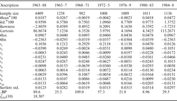
The data set is studied in subsample periods 1963±7, 1968±71, 1972±5, 1976±9, 1980±3 and 1984±8. The summary statistics of the daily returns for all subsamples are presented in Table I. The daily returns are calculated as the log di€erences of the Dow level. None of the subperiods except the 1984±8 period show signi®cant skewness and excess kurtosis.

The ®rst ten autocorrelations are also given in the rows labelledr_n. The Barlett standard errors from these series are also reported in Table I. All periods show some evidence of autocorrelation in the ®rst lag. The Ljung±Box±Pierce statistics are shown in the last row. These are calculated Table I. Summary statistics of the log ®rst di€erenced daily DJIA series January 1963±June 1988 Description 1963±88 1963±7 1968±71 1972±5 1976±9 1980±83 1984±8 Sample size 6409 1258 982 1008 1009 1011 1136 Mean*100 0.0187 0.0267 ÿ0.0019 ÿ0.0042 ÿ0.0023 0.0418 0.0472 Std.*100 0.9598 0.5780 0.7503 1.0960 0.7709 0.9775 1.3752 Skewness ÿ2.8059 0.0589 0.4932 0.2091 0.1650 0.3592 ÿ5.7253 Kurtosis 86.8674 7.1234 6.3526 3.9791 4.1694 4.3425 113.2671 Max 0.0967 0.0440 0.0495 0.0460 0.0436 0.0478 0.0967 Min ÿ0.2563 ÿ0.0293 ÿ0.0319 ÿ0.0357 ÿ0.0304 ÿ0.0359 ÿ0.2563 r₁ 0.1036 0.1212 0.2929 0.2118 0.1130 0.0470 0.0126 r2 ÿ0.0390 0.0269 ÿ0.0024 ÿ0.0531 0.0090 0.0480 ÿ0.1051 r3 ÿ0.0083 0.0243 0.0046 ÿ0.0099 0.0197 ÿ0.0228 ÿ0.0172 r4 ÿ0.0231 0.0480 0.0485 ÿ0.0260 ÿ0.0188 ÿ0.0361 ÿ0.0466 r₅ 0.0247 0.0267 0.0248 ÿ0.0627 ÿ0.0051 ÿ0.0243 0.1015 r₆ ÿ0.0098 0.0153 ÿ0.0639 ÿ0.0360 ÿ0.0530 0.0293 0.0058 r₇ 0.0065 0.0014 ÿ0.0314 0.0072 0.0114 ÿ0.0130 0.0234 r₈ ÿ0.0029 0.0396 0.1087 ÿ0.0054 ÿ0.0632 ÿ0.0164 ÿ0.0151 r₉ ÿ0.0133 0.0107 0.0086 ÿ0.0487 0.0216 0.0099 ÿ0.0230 r₁₀ ÿ0.0133 ÿ0.0064 ÿ0.0619 ÿ0.0048 0.0166 ÿ0.0205 ÿ0.0131 Bartlett std. 0.0125 0.0282 0.0319 0.0315 0.0315 0.0314 0.0297 LBP 89.6 25.3 109.0 57.3 21.8 8.96 29.5 w2 005…10† 18.307

Notes:r1, . . .,r10are the ®rst ten autocorrelations of each series. LBP refers to the Ljung±Box±Pierce statistic and it is

for the ®rst ten lags and are distributed w2_{(10) under the null of identical and independent} observations. Five series out of six give strong rejection of the null hypothesis of identical and independent observations.

ESTIMATOR TECHNIQUES

Letp_t, tˆ1, 2, . . . ,Tbe the daily Dow series. The return series are calculated byr_tˆlog(p_t) 7log(p_t71). Letmn

t and vkt denote the timetvalue of a price average rule of lengthnand the volume average of lengthk, respectively.mn

t andvkt are calculated by mn_t ˆ …1=n†Xnÿ1

iˆ0

p_tÿi vk_t…1=k†Xkÿ1 jˆ0

vol_tÿj …3†

The buy and sell signals for the price average rule are calculated1_by

sn1_t ;n2ˆmn1_t ÿmn2_t …4†

wheren1 andn2 are the short and the long moving averages, respectively. The rule used in this paper is (n1,n2)ˆ(1,200) wheren1 andn2 are in days. This rule is widely used in practice. The test regressions for the OLS and GARCH-M models of this rule are

r_t ˆa₀‡Xp iˆ1 b_isn1_tÿ;₁n2‡e_t e_t ID 0 ;s2_t …5† and r_t ˆa₀‡Xp iˆ1 b_isn1_tÿ;₁n2‡gh1_t=2‡e_t …6† wheree_tN(0,h_t) andh_t ˆd₀‡d₁h_tÿ1‡d₂e2 tÿ1.

The indicator variable for the volume average rule is calculated by Ik1_t ;k2ˆ 1; …vk1t ÿvk2t †40

ÿ1; …vk1

t ÿvk2t †40

…7† The volume rule used in this paper is (k1,k2)ˆ(1,10) wherek1 andk2 are in days.

The linear test regression for the technical trading rule with volume indicator is r_t ˆa₀‡a₁I_tk1_ÿ;₁k2‡Xp

iˆ1

b_isn1_tÿ;_in2‡e_t …8† 1_{The analysis above generates continuous buy±sell signals. An alternative way to construct the buy±sell signals is to}

construct an indicator function given 1 whensn1;n2

t 40 (the short moving average is above the long) andÿ1 otherwise.

wheree_t ID…0;s2

t†. In case of the GARCH-M(1,1) process the test model is written as r_t ˆa₀‡a₁I_tk1_ÿ;₁k2‡Xp

iˆ1

b_isn1_tÿ;₁n2‡gh1_t=2‡e_t …9† wheree_tN(0,h_t) andh_t ˆd₀‡d₁h_tÿ1‡d₂e2

tÿ1.

There are numerous non-parametric regression techniques available such as ¯exible Fourier forms, non-parametric kernel regression, wavelets, spline techniques and arti®cial neural networks. Here, a class of arti®cial neural network models, namely the single-layer feedforward networks, is used. The justi®cation for this choice is that the rate of convergence of these networks does not depend on the dimensionality of the input space. Recently, Horniket al. (1994) have shown that single hidden-layer feedforward networks can approximate unknown functions and their derivatives with error decreasing at rates as fast asdÿ1=2_{and that the dimension of the input} space,p, does not a€ect the rate of approximation, but only the constants of proportionality. This is in sharp contrast to the properties of the standard kernel and series approximants. This is an advantage in terms of having desirable estimators in small samples. The single-layer feedforward network regression model with lagged buy and sell signals and withdhidden units is written as

r_t ˆa₀‡Xd jˆ1 b_jG a_1j‡Xp iˆ1 g_ijsn1_tÿ;₁n2 ! ‡e_t e_t ID 0 ;s2_t …10†

whereGis the known activation function which is chosen to be the logistic function. This choice is common in the arti®cial neural networks literature. The test regression model with the volume indicator is written as r_t ˆa₀‡Xd jˆ1 b_jG a_1j‡a_2jI_tk1_ÿ;₁k2‡Xp iˆ1 g_ijsn1_tÿ;₁n2 ! ‡e_t e_t ID 0 ;s2_t …11† Many authors have investigated the universal approximation properties of neural networks (Gallant and White, 1988, 1992; Cybenko, 1989; Funahashi, 1989; Hecht-Nielson, 1989; Hornik, Stinchcombe and White, 1989, 1990). Using a wide variety of proof strategies, all have demonstrated that under general regularity conditions, a suciently complex single hidden-layer feedforward network can approximate any member of a class of functions to any desired degree of accuracy where the complexity of a single hidden-layer feedforward network is measured by the number of hidden units in the hidden layer. For an excellent survey of the feedforward and recurrent network models, the reader may refer to Kuan and White (1994).

To compare the performance of the regression models in (5), (6), (8), (9), (10) and (11) the linear regression

r_t ˆa‡Xp iˆ1

b_ir_tÿ1‡e_t e_t ID 0 ;s2_t …12† is used with the lagged returns as the benchmark model. The out-of-sample forecast performance of equations in (5), (6), (8), (9), (10) and (11) are measured by the ratio of their mean square prediction errors (MSPEs) to that of the linear benchmark model in equation (12).

A number of papers in the literature suggest that conditional heteroscedasticity may be important in the improvement of the forecast performance of the conditional mean. For this reason, the MSPE of the GARCH-M(1,1) model with lagged returns

r_t ˆa‡Xp iˆ1

b_ir_tÿ1‡gh_t1=2‡e_t e_t N…0;h_t† h_t ˆd₀‡d₁h_tÿ1‡d₂e2_tÿ1 …13† is compared to that of the benchmark model in equation (12).

The out-of-sample forecast performance of the single-layer feedforward network model with lagged returns r_t ˆa₀‡Xd jˆ1 b_jG a_j‡Xp iˆ1 g_ijr_tÿ1 ! ‡e_t e_t ID 0 ;s2_t …14†

is also compared to that of the benchmark model in equation (12).

Feedforward network regression models require a choice for the number of hidden units in a network. Let o_t ˆa₀‡Xd jˆ1 b_jG a_j‡Xp iˆ1 g_ijx_tÿi ! …15† wherex_t7iis either past returns (equation (14)) or past buy±sell signals (equations (10) and (11)). The cross-validated performance measure is formally de®ned2_as

C_T…d† Tÿ1XT tˆ1

r_t ÿo^d_T…t† h i2

…16† whereo^d_T…t†ignores information from thetth observation and consequently provides a measure of network performance superior to average squared error.

A completely automatic method for determining network complexity appropriate for any speci®c application is given by choosing the number of hidden unitsdÃ_Tto be the smallest solution to the problem

min_d2N

TCT…d† …17†

whereN_Tis some appropriate choice set. Here, we setN_Tˆ{1, 2, . . ., 10}. The number of lags for the past buy±sell signals in each regression is chosen to bepˆ1, 2 or 3 lags. In models with volume indicator, the ®rst lag of the volume indicator is always used as a regressor. For each one-step-ahead forecast observation, the feedforward network regression is re-estimated and the optimal network complexity is determined according to the cross-validated performance measure. Accordingly, a di€erent model may be indicated by the cross-validated performance measure at di€erent forecast horizons. A rolling-sample approach is used so that same number of observations are used as the in-sample observations at every one-step-ahead prediction. The 2_{Moody and Utans (1994) also use cross-validated performance measure within the context of corporate bond rating}

maximum number of hidden units (N_Tˆ10) and the maximum number of lags (pˆ3) in a given feedforward regression is chosen according to the computational limitations.

EMPIRICAL RESULTS

For each subsample the out-of-sample predictive performances of the benchmark and test models are examined. For each subsample the forecast horizon is chosen to be the last one-third of each data set. There are two advantages of constructing the forecast horizon from six di€erent subsamples. The ®rst is to avoid spurious results as a result of data-snooping problems or sample-speci®c conditions. The second is that it enables us to analyse the performance of the technical trading rules under di€erent market conditions. This is particularly important in observing the performance of these rules in trendy versus sluggish market conditions in which there is no clear trend in either direction. Out-of-sample forecasts are completely ex ante by using only the information actually available.

Let MSPEt_{AND MPSE}b _{be the mean square prediction errors of the test and benchmark} models, respectively. To measure the out-of-sample performance between the test and bench-mark models, the ratio of the mean square prediction errors,MSPEt_/MSPEb_{is used.MSPE}t_/ MSPEb_{is less than one if the test model provides more accurate predictions. Similarly, the ratio is} greater than one if the predictions of the test model are less accurate relative to the benchmark model.

Empirical results with past returns

The MSPEs of the benchmark (equation (12)), GARCH-M(1,1) and the feedforward network models with past returns are presented in Table II. The MSPEs of the benchmark model are reported in levels. MSPEs of the GARCH-M(1,1) and the feedforward network models are reported as a ratio to the MSPEs of the benchmark model. All three speci®cations are estimated for three lags of the past returns.

Table II reports that the out-of-sample forecast performance of the GARCH-M(1,1) model does not outperform the benchmark model. The di€erence between the average MSPEs of both models is less than 10%. The GARCH-M(1,1) model, however, has more accurate average sign predictions.

One further consideration is to exploit any potential non-linearities that might exist in the conditional mean which might add to the forecasting power of the past returns. The results of the model in equation (14) with feedforward network estimation are presented in the last two columns of Table II. In the majority of the subperiods, the feedforward network model provides smaller MSPEs in comparison to the benchmark and the GARCH-M(1,1) models. The results are especially suggestive in the fourth and ®fth periods where the neural network model performs considerably better than the other models in terms of MSPEs and sign predictions. The average forecast improvement of the feedforward network model is about 2.5% and provides more accurate sign predictions than the GARCH(1,1) model. The results also do not seem to be sensitive to the choice of lag length.

Overall, the results of the feedforward network regression with past returns indicate forecast improvement over the benchmark model and the GARCH-M(1,1) speci®cation. Furthermore, both GARCH-M(1,1) and feedforward network models provide more accurate average sign predictions relative to the benchmark parametric model.

Empirical results with past buy±sell signals of the moving average rules

The predictability of the current returns with the past buy±sell signals of the moving average rules are investigated with two di€erent moving average rules. These are the (1,200) rule without the volume indicator and the (1,200) rule with 10-day volume average indicator. For convenience, we will call these rules A and B, respectively.

The results with rule A are presented in Table III. Both OLS and the GARCH-M(1,1) speci®cations provide slight improvements over the benchmark model with respect to their average MSPEs. The GARCH-M(1,1) model, however, provides higher average sign predictions relative to the OLS model. The last two columns of Table III are devoted to the feedforward network regression results with past buy±sell signals. Again the feedforward network model outperforms its competitors in terms of MSPEs and sign predictions, especially in the ®rst and ®fth periods. Overall, it provides smaller MSPEs than the GARCH-M(1,1) model and the feed-foward network model has more accurate sign predictions. Also, the results seen insensitive to the choice of lag length. Comparing the results of Tables II and III we can see that it is the feed-forward network model that improves with the use of moving average rules, whereas the OLS and the GARCH-M(1,1) models do not seem to perform di€erently between the two cases.

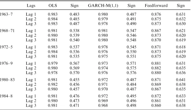
In Table IV, rule B is studied. The only di€erence between rules A and B is that rule B accommodates for the volume indicator as an additional regressor. This measures any additional forecast gain attained from the volume variable. The test models for the linear models are presented in equations (5), (6), (8) and (9). The non-linear conditional speci®cation is given in equations (10) and (11). In Table IV, the OLS and the GARCH-M(1,1) speci®cations attain an Table II. MSPEs of the models with past returns

Lags OLS Sign GARCH-M(1,1) Sign Feedforward Sign

1963±7 Lag 1 [0.4849] 0.466 1.000 0.467 0.984 0.500 Lag 2 [0.4866] 0.465 0.997 0.467 0.981 0.511 Lag 3 [0.4864] 0.462 0.996 0.463 0.983 0.513 1968±71 Lag 1 [0.4290] 0.533 0.995 0.534 0.994 0.541 Lag 2 [0.4263] 0.523 0.996 0.533 0.990 0.542 Lag 3 [0.4256] 0.511 0.998 0.532 0.982 0.543 1972±5 Lag 1 [1.6164] 0.531 0.995 0.533 0.994 0.535 Lag 2 [1.6151] 0.510 0.996 0.521 0.990 0.545 Lag 3 [1.5556] 0.511 0.998 0.518 0.982 0.543 1976±9 Lag 1 [0.6938] 0.551 0.998 0.554 0.971 0.585 Lag 2 [0.6929] 0.567 0.997 0.568 0.967 0.583 Lag 3 [0.6926] 0.563 0.998 0.565 0.973 0.581 1980±83 Lag 1 [1.1522] 0.431 0.996 0.451 0.968 0.533 Lag 2 [1.1599] 0.433 0.995 0.457 0.943 0.554 Lag 3 [1.1618] 0.430 0.999 0.451 0.959 0.553 1984±8 Lag 1 [4.3259] 0.465 1.000 0.467 0.984 0.510 Lag 2 [4.3495] 0.466 0.997 0.467 0.981 0.512 Lag 3 [4.3743] 0.463 0.996 0.465 0.983 0.521

Notes: The numbers in brackets are the MSPEs of the benchmark model in levels. MSPEs of the GARCH-M(1,1) and the feedforward network models are reported as a ratio to the MSPEs of the benchmark model. MSPEs of the benchmark model are1074_{. `Sign' refers to the average sign predictions in the forecast horizon}

Table III. The ratio of the MSPEs of the models with past buy±sell signals to the MSPEs of the benchmark model (moving average rule without volume indicator)

Lags OLS Sign GARCH-M(1,1) Sign Feedforward Sign

1963±7 Lag 1 0.997 0.467 0.994 0.469 0.911 0.571 Lag 2 0.998 0.467 0.994 0.468 0.913 0.573 Lag 3 0.995 0.465 0.991 0.465 0.911 0.571 1968±71 Lag 1 0.996 0.536 0.990 0.534 0.905 0.581 Lag 2 0.995 0.527 0.991 0.534 0.908 0.582 Lag 3 0.998 0.514 0.992 0.537 0.906 0.587 1972±5 Lag 1 0.994 0.534 0.993 0.538 0.905 0.591 Lag 2 0.993 0.515 0.991 0.522 0.901 0.593 Lag 3 0.991 0.516 0.990 0.520 0.900 0.590 1976±9 Lag 1 0.990 0.556 0.989 0.555 0.909 0.597 Lag 2 0.991 0.564 0.987 0.570 0.907 0.598 Lag 3 0.994 0.568 0.988 0.567 0.904 0.599 1980±83 Lag 1 0.994 0.435 0.993 0.454 0.900 0.600 Lag 2 0.995 0.431 0.995 0.459 0.901 0.601 Lag 3 0.995 0.435 0.996 0.455 0.903 0.602 1984±8 Lag 1 0.994 0.464 0.990 0.469 0.904 0.597 Lag 2 0.993 0.463 0.991 0.468 0.905 0.598 Lag 3 0.995 0.462 0.992 0.467 0.901 0.599

Table IV. The ratio of the MSPEs of the models with past buy±sell signals to the MSPEs of the benchmark model (moving average rule with volume indicator)

Lags OLS Sign GARCH-M(1,1) Sign Feedforward Sign

1963±7 Lag 1 0.983 0.483 0.980 0.487 0.876 0.631 Lag 2 0.984 0.485 0.979 0.491 0.875 0.632 Lag 3 0.983 0.487 0.978 0.490 0.873 0.630 1968±71 Lag 1 0.981 0.538 0.981 0.547 0.867 0.621 Lag 2 0.980 0.539 0.980 0.546 0.873 0.620 Lag 3 0.981 0.540 0.980 0.548 0.870 0.619 1972±5 Lag 1 0.983 0.537 0.978 0.545 0.871 0.618 Lag 2 0.984 0.536 0.976 0.550 0.873 0.619 Lag 3 0.981 0.535 0.975 0.551 0.875 0.620 1976±9 Lag 1 0.979 0.567 0.973 0.571 0.881 0.631 Lag 2 0.980 0.569 0.974 0.575 0.882 0.635 Lag 3 0.978 0.570 0.976 0.576 0.880 0.636 1980±83 Lag 1 0.981 0.455 0.972 0.487 0.871 0.641 Lag 2 0.982 0.456 0.971 0.484 0.869 0.638 Lag 3 0.980 0.457 0.970 0.487 0.867 0.635 1984±8 Lag 1 0.981 0.476 0.972 0.495 0.872 0.633 Lag 2 0.980 0.473 0.969 0.496 0.861 0.631 Lag 3 0.981 0.471 0.968 0.498 0.860 0.638

average of 2% improvement over the benchmark model. Furthermore, the GARCH-M(1,1) speci®cation has more accurate sign predictions in comparison to the OLS model. The neural network model improves both on the MSPEs and sign predictions when compared with the OLS and GARCH-M(1,1) models, especially for the ®rst, ®fth and sixth periods. Furthermore, as before, the choice of lag length does not seem to matter. In feedforward network speci®cations, rule B attains an average of 12% forecast gain over the benchmark model. This additional forecast gain is approximately 50% more than the forecast performance of the feedforward networks without the volume indicator. Moreover, the feedforward network models provide an average of 62% correct sign predictions. It is noticeable that the OLS and GARCH-M(1,1) models also show improvement with the volume indicator over their previous performance from the comparison of Tables II±IV.

CONCLUSIONS

This paper has used the daily Dow Jones Industrial Average Index from January 1963 to June 1988 to examine the linear and non-linear predictability of stock market returns with some simple technical trading rules which utilize price and volume averaging. In linear conditional mean speci®cations, these rules do not provide forecast gains over the linear benchmark model with past returns. The GARCH-M(1,1) model, however, provides a higher percentage of sign predictions over the OLS model when past buy±sell signals of the moving average rules and the volume indicator are used as regressors. In non-linear conditional mean speci®cations, the feedforward network model does improve on the benchmark model. In addition, the volume indicator adds additional forecast accuracy. The technical trading rules used in this paper are very popular and very simple. The results here suggest that it is worth while to investigate more elaborate rules and the pro®tability of these rules after accounting for transaction costs and brokerage fees.

ACKNOWLEDGEMENTS

We thank the editors and two anonymous referees for their constructive comments. Both authors thank to the Social Sciences and Humanities Research Council of Canada for support. Ramazan GencËay also thanks the Natural Sciences and Engineering Research Council of Canada for its support.

REFERENCES

Blume, L., Easley, D. and O'Hara, M., `Market statistics and technical analysis: The role of volume',

Journal of Finance,49(1994), 153±181.

Brock, W. A., Lakonishok, J. and LeBaron, B., `Simple technical trading rules and the stochastic properties of stock returns',Journal of Finance,47(1992), 1731±1764.

Campbell, J. Y., Grossman, S. J. and Wang, J., `Trading volume and serial correlation in stock returns',

Quarterly Journal of Economics,108(1993), 905±940.

Chopra, N., Lakonishok, J. and Ritter, J. R., `Performance measurement methodology and the question of whether stocks overreact',Journal of Financial Economics,31(1992), 235±268.

Colby, R. W. and Meyers, T. A., `The Encyclopedia of Technical Market Indicators', Business One Irwin, (1988).

Conrad, J. S., Hameed, A. and Niden, C., `Volume and autocovariances in short-horizon individual security returns',Journal of Finance,49(1994), 1305±1329.

Conrad, J. and Kaul, G., `Time-variation in expected returns',Journal of Business,61(1988), 409±425. Cutler, D. M., Poterba, J. M. and Summers, L. H., `Speculative dynamics',Review of Economic Studies,58

(1991), 529±546.

Cybenko, G., `Approximation by superposition of a sigmoidal function',Mathematics of Control, Signals

and Systems,2(1989), 303±314.

De Bondt, W. F. M. and Thaler, R. H., `Does the stock market overreact',Journal of Finance,40(1985), 793±805.

Engle, R. F., Lilien, D. and Robins, R. P., `Estimating time varying risk premia in the term structure: the ARCH-M model',Econometrica,55(1987), 391±407.

Fama, E. F., `The behavior of stock market prices',Journal of Business,38(1965), 34±105.

Fama, E. F., `Ecient capital markets: A review of theory and empirical work',Journal of Finance,25 (1970), 383±417.

Fama, E. F., `Ecient capital markets: II',Journal of Finance,46(1991), 1575±1617.

Fama, E. F. and French, K. R., `Permanent and temporary components of stock prices',Journal of Political

Economy,98(1986), 246±274.

Fisher, L., `Some new stock-market indexes',Journal of Business,39(1966), 191±225.

French, K. R. and Roll, R., `Stock return variances: The arrival of information and the reaction of traders',

Journal of Financial Economics,17(1986), 5±26.

Funahashi, K.-I., `On the approximate realization of continuous mappings by neural networks',

Neural Networks,2(1989), 183±192.

Gallant, A. R. and White, H., `There exists a neural network that does not make avoidable mistakes',

Proceedings of the Second Annual IEEE Conference on Neural Networks, San Diego, CA, I.657-I.644,

New York: IEEE Press, 1988.

Gallant, A. R. and White, H., `On learning the derivatives of an unknown mapping with multilayer feedforward networks',Neural Networks,5(1992), 129±138.

Hecht-Nielsen, R., `Theory of the backpropagation neural networks', Proceedings of the International

Joint Conference on Neural Networks, Washington, DC, I.593-I.605, New York: IEEE Press, 1989.

Hornik, K., Stinchcombe, M. and White, H., `Multilayer feedforward networks are universal approximators',Neural Networks,2(1989), 359±366.

Hornik, K., Stinchcombe, M. and White, H., `Universal approximation of an unknown mapping and its derivatives using multilayer feedforward networks',Neural Networks,3(1990), 551±560.

Hornik, K., Stinchcombe, M., White, H. and Auer, P., `Degree of approximation results for feedforward networks approximating unknown mappings and their derivatives', UCSD discussion paper, 1994.

Jegadeesh, N., `Evidence of predictable behavior of security returns', Journal of Finance, 45 (1990), 881±898.

Jensen, M. C., `Some anomalous evidence regarding market eciency',Journal of Financial Economics,6 (1978), 95±101.

Karpov, J. M., `The relation between price changes and trading volume: A survey',Journal of Financial and

Quantitative Analysis,22(1987), 109±126.

Kuan, C.-M. and White, H., `Arti®cial neural networks: An econometric perspective', Econometric

Reviews,13(1994), 1±91.

Lehmann, B. N., `Fads, martingales and market eciency',Quarterly Journal of Economics,105(1990), 1±28.

Lo, A. W. and MacKinlay, A. C., `Stock market prices do not follow random walks: Evidence from a simple speci®cation test',Review of Financial Studies,1(1988), 41±66.

Lo, A. W. and MacKinlay, A. C., `When are contrarian pro®ts due to stock market overreaction?'Review of

Financial Studies,3(1990), 175±205.

Moody, J. and Utans, J., `Architecture selection strategies for neural networks: Application to corporate bond rating prediction', in Refenes, A. P. N. (ed.),Neural Networks in the Capital Markets, New York: John Wiley.

Nelson, D. B., `Conditional heteroscedasticity in asset returns: A new approach',Econometrica,59(1991), 347±370.

Poterba, J. M. and Summers, L. H., `Mean reversion in stock prices: Evidence and implications',Journal of

Financial Economics,22(1988), 27±59.

Authors' biographies:

Ramazan GencËayis a Professor in the Economics Department at the University of Windsor. His areas of specialization are non-linear time series modelling, ®nancial forecasting and the detection of chaotic dynamics from observed data. Some of his publications have appeared in theJournal of the American

Statistical Association,Physica D,Journal of Nonparametric Statistics,Journal of Applied Econometrics,

Journal of ForecastingandJournal of Empirical Finance.

Thanasis Stengosis a professor in the Economics Department at the University of Guelph. His areas of specialization are nonparametric econometrics, non-linear time series modelling and the defection of chaotic dynamics from observed data. Some of his publications have appeared in Review of Economic Studies,

Journal of Monetary Economics,International Economic Review,European Economic ReviewandJournal of

Econometrics.

Authors' addresses:

Ramazan GencËay, Department of Economics, University of Windsor, 401 Sunset Avenue, Windsor, Ontario, N9B 3P4, Canada.