Generation of collision-free trajectories for a quadrocopter fleet:
A sequential convex programming approach
Federico Augugliaro, Angela P. Schoellig, and Raffaello D’Andrea
Abstract— This paper presents an algorithm that generates collision-free trajectories in three dimensions for multiple ve-hicles within seconds. The problem is cast as a non-convex op-timization problem, which is iteratively solved using sequential convex programming that approximates non-convex constraints by using convex ones. The method generates trajectories that ac-count for simple dynamics constraints and is thus independent of the vehicle’s type. An extensive a posteriorivehicle-specific feasibility check is included in the algorithm. The algorithm is applied to a quadrocopter fleet. Experimental results are shown.
I. INTRODUCTION
When working with multiple flying vehicles, critical phases (such as takeoff and landing) can benefit strongly from the use of an algorithm that allows for collision-free trajectory planning. In this paper, we propose a simple method based on sequential convex programming (SCP) [1] to plan trajectories for multiple vehicles in 3D space. The goal is to transition from an initial set of states – consisting of position, velocity and acceleration of each vehicle – to a final one, while maintaining a minimum distance between vehicles and satisfying additional trajectory constraints. The approach is applied to quadrocopters (Fig. 1), but can be readily used for different platforms by modifying the constraints. This work was inspired by the work on SCP by Wang at al. [2]. Sophisticated methods for generating quadrocopter tra-jectories that account for vehicle constraints can be found e.g. in [3] and [4]. In this paper, we minimize the total thrust required to fly the trajectories and introduce avoidance constraints to couple the trajectories of multiple vehicles. We assume that the vehicle is able to track the generated trajec-tories (by means of an appropriate controller), provided that they satisfy a feasibility check. Decoupling the extensive fea-sibility check from the trajectory planning algorithm results in a simple and flexible method for generating collision-free trajectories for multiple vehicles within seconds. A method for aircraft trajectory planning with avoidance constraints that also exploits simplified dynamics and constraints can be found in [5]. Two recent surveys, [6] and [7], present various research on motion planning for UAVs.
In robotics, the generation of trajectories with avoidance constraints has been extensively studied. According to [8], two different approaches exist: planning and reacting. The planned approach generates feasible paths ahead of time; whereas the reactive approach typically uses an online colli-sion avoidance system to respond to dangerous situations, The authors are with the Institute for Dynamic Systems and Control, ETH Zurich, Switzerland. {faugugliaro, aschoellig, rdandrea}@ethz.ch
as in [9]. The two methods can also be combined. This work focuses on a planned approach. The planning can be performed in a decentralized fashion [10] or centralized [11] as in this paper. Trajectory generation with avoidance con-straints for multiple vehicles has been studied, among others, for differential-drive robots [12], underwater vehicles [13] and aircrafts [14]. Collision-free trajectories generation is also central to pattern formation research [15], [16].
Our approach results in trajectories for multiple vehicles that are simultaneously executed. Although it is straightfor-ward to account for the presence of obstacles by imposing minimum distances between vehicles and given obstacle points, in the following sections we assume that the envi-ronment is obstacle-free.
This paper is organized as follows: In Section II, we state the collision-free trajectory generation problem as an optimization problem entailing non-convex constraints. Section III explains how SCP allows us to approximate non-convex constraints by using convex ones, such that the framework of quadratic programming can be used to effectively solve the problem. Section IV describes the overall algorithm, including ana posteriorifeasibility check of the resulting trajectories. Finally, Section V presents experimental results and discusses the computational effort of the algorithm. A video demonstrating collision-free quadro-copter motion is attached to this work and found online
athttp://youtu.be/wwK7WvvUvlI. Enough detail is
given such that the algorithm can be easily implemented on other platforms.
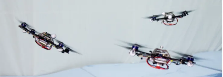
II. TRAJECTORY OPTIMIZATION FOR MULTIPLE VEHICLES WITH AVOIDANCE CONSTRAINTS The goal is to generate collision-free trajectories for N vehicles, allowing a transition in a given time T from an initial set of states to a final set of states (position, veloc-ity, and acceleration). The trajectories must satisfy various
Fig. 1. Multiple quadrocopters flying collision-free trajectories in the ETH Flying Machine Arena.
constraints, including physical limits of the vehicle, space boundaries and avoidance constraints.
In this section, we state the trajectory planning problem as an optimization problem. We thus define an objective func-tion that we want to minimize, a free optimizafunc-tion variable, simple dynamics describing the evolution of the trajectories, and inequality and equality constraints. The proposed method may be used to generate trajectories for any arbitrary type of vehicle. However, the vehicle type influences the choice of some constraints. We will comment on this at various points in the text.
A. Trajectory dynamics
In the following, we denote withpi[k]∈R3the position of
vehiclei at discrete timesk∈ {1, . . . , K}. Its velocity and acceleration are indicated by vi[k] and ai[k], respectively.
The trajectory of vehicle i obeys the simple discretized dynamics equations:
vi[k+ 1] =vi[k] +h ai[k], (1) pi[k+ 1] =pi[k] +h vi[k] +
h2
2 ai[k], (2)
where his the discretization time step.
B. Optimization variable
The optimization variable χ ∈ R3N K consists of the
vehicles’ accelerations at each time stepk. From (1) and (2), it follows that the position and velocity of each vehicle at any timekare affine functions ofχ. The velocity of vehicle iat time k, k >1,is given by
vi[k] =vi[1] +h ai[1] +ai[2] +. . .+ai[k−1], (3)
while the position is expressed by
pi[k] =pi[1] +h(k−1)vi[1] (4) +h2
2 (2k−3)ai[1] + (2k−5)ai[2] +. . .+ai[k−1]
. Expressions (3) and (4) can be cast into matrix form, mapping acceleration to velocity and position, for later use when defining the constraints.
C. Objective function
The optimality criterion is chosen to be the sum of the total thrust at each time step, which, for a quadrocopter, is given by f0= N X i=1 K X k=1 kai[k] +~gk22, (5)
where~g is the gravity vector [3]. Based on our experience, this choice results in smooth trajectories. Equation (5) can be expressed as a quadratic function of the optimization variable χ, resulting in
f0(χ) =χTP χ+qTχ+r. (6)
D. Convex constraints
Initial and final states are given for each vehicle. This in-troduces equality constraints on the initial and final position, velocity, and acceleration. Furthermore, to meet a vehicle’s physical constraints, velocity, acceleration and jerk (the third derivative of the position) can be constrained. When dealing with quadrocopters, it is necessary to introduce constraints on acceleration and jerk. Finally, space boundaries limit the allowable position in space. The aforementioned constraints can be expressed by affine functions of χ in the form of equality and inequality constraints:
Aeqχ=beq, (7) Ainχbin, (8)
where the inequalities are expressed element-wise. Below, we introduce these constraints in more detail, highlighting those specific to quadrocopters.
1) Initial and final states: As stated above, position, velocity, and acceleration are defined for each vehicle at time k= 1andk=K. Note that the initial position and velocity are already taken into account in (3) and (4). We must thus introduce 12 constraints for each vehicle accounting for the initial acceleration, and final position, velocity and acceleration in three dimensions. This results in the following matrices
Aeq∈R12N×3N K, beq ∈R12N. (9)
2) Position: The working space is usually limited, adding position constraints as follows:
pmin,l ≤pi,l[k]≤pmax,l, l∈ {x, y, z}, ∀i, k. (10)
In our case, this results in6N K inequality constraints.
3) Velocity: Similarly, boundaries on velocity can be specified. However, in limited indoor space operations the quadrocopter can never reach its maximum velocity. There-fore, velocity is not constrained here.
4) Acceleration: On a quadrocopter, the collective thrust is limited by a minimum and a maximum thrust value, de-noted by fmin andfmax, respectively. Taking quadrocopter
dynamics into account, the condition reads as fmin≤
q
(ai,x)2+ (ai,y)2+ (ai,z+g)2≤fmax, (11)
which results in a quadratic constraint. Instead, to simplify and speed up the solution to the problem, we decouple the single directions by constraining each coordinate separately. We thus have:
amin,l ≤ai,l[k]≤amax,l l∈ {x, y, z}, ∀i, k, (12)
where, in our case, the limits are chosen such that (11) is satisfied for the extremal case. We thus have:
q
(amax,x)2+ (amax,y)2+ (amax,z+g)2≤fmax, (13) g+amin,z≥fmin . (14)
This fits the affine formulation presented above and con-tributes with6N K additional inequality constraints.
5) Jerk: Analogously, for each coordinate we derive jerk constraints. Bounded jerk implies continuity in the accelera-tion, which for a quadrocopter corresponds to continuity in the attitude [3]. In our case, constraining the jerk is therefore necessary to obtain feasible trajectories. We thus have,
jmin,l ≤ji,l[k]≤jmax,l l∈ {x, y, z}, ∀i, k, (15)
where j[k] = (a[k]−a[k−1])/h. This adds 6N(K−1) inequality constraints to the problem.
E. Non-convex collision avoidance constraints
The vehicles must not collide during the transition from the initial states to the final states. This is captured by the following non-convex constraints:
kpi[k]−pj[k]k2≥R, ∀i, j, i6=j, ∀k, (16)
which guarantee a minimum distance R between vehicles at each timek.
In this section, we stated an optimization problem, which allows the generation of trajectories for multiple vehicles from a set of initial states to a set of final states. Because of the collision avoidance constraint (16), the problem is non-convex.
In the following section, we introduce SCP, a local op-timization method that allows the approximation of non-convex constraints.
III. SEQUENTIAL CONVEX PROGRAMMING Sequential convex programming is a local optimization method for non-convex problems [1]. The idea is to replace non-convex constraints with convex approximations around a previous solution χq. The convex problem is solved
iteratively, starting from an initial guess χ0. The method iterates until a stop condition is satisfied. SCP is a heuristic
method and may fail to find the optimal solution. Moreover, the result depends on the initial guess χ0. Nevertheless, according to [1] it often works well and finds a feasible solution with satisfactory, if not optimal, objective value. This was confirmed in our numerous experiments (see Sec. V for details).
A. Approximated collision avoidance constraints
The collision avoidance constraint (16) at iteration(q+ 1) is linearized around the previous solution χq using a
first-order Taylor expansion pq i[k]−p q j[k] 2+ (17) ηT pi[k]−pj[k]− pqi[k]−p q j[k] ≥R with η= p q i[k]−p q j[k] pq i[k]−p q j[k] 2 ,
where pqi is the position of vehicle i corresponding to the solution χq, cf. (4). Equation (17) can be cast into affine
form, addingNcKinequality constraints withNc=N(N− 1)/2.
B. Resulting quadratic program
With approximation (17), the non-convex trajectory plan-ning problem can be formulated as a quadratic program, since the objective function is quadratic and the constraint functions are affine [17]:
minimize χTP χ+qTχ+r subject to Aeqχ=beq (18) Ainχbin, where χ ∈ R3N K, A eq ∈ R12N×3N K, Ain ∈ RM×3N K, withM = 23.5KN−6N+ 0.5KN2.
Quadratic programs can be solved very efficiently using existing software packages such as [18]. Further, if the optimization problem is feasible (i.e., if there exists χ that satisfy the constraints), then there exists a local minimum that is globally optimal. In practice, convex optimization problems are tractable for a large number (hundreds, if not thousands) of decision variables and constraints.
C. The sequential convex programming loop
The SCP loop consists of the following steps:
1) Problem parameters: First, the discretization step h is chosen. With the given trajectory duration T, we have K=T /h+ 1, wherehis chosen such thatK∈N.
2) Starting point: As explained above, the SCP algorithm iteratively solves a convex problem around a previous so-lution χq. It thus requires a starting point χ0, which is chosen to be the solution to (18) without the avoidance constraint (17). This is motivated by the fact that the resulting trajectories of the problem without avoidance constraints are often close to the ones of the actual problem.
3) Stopping conditions: The problem is iterated with χq
being the solution to the approximate QP (18) at iterationq, until the following conditions are satisfied:
1) χq is an optimal solution of the approximate convex
problem.
2) χq fulfills the non-convex avoidance constraint (16).
3) Convergence in the objective value is achieved, i.e. |f0(χq−1)−f0(χq)|< , whereis a tuning parameter. In our setup, the problem converges in less than four iterations. Results are shown in Sec. V-A.2.
D. Discussion
The solution returned by the SCP algorithm (if any exists) results in trajectories that fulfill the constraints introduced in Sec. II-D and Sec. II-E. However, this method has two main limitations.
First, some constraints (in our case, the jerk and acceler-ation) are only approximations of vehicles’ physical limits, and there is therefore no guarantee that the trajectories are feasible. Including true vehicle dynamics (even if simplified) results in a larger problem dimension and in a potentially nonlinear problem. Both effects lead to a much longer solution time. In addition, the definition of the dynamics and constraints is vehicle specific. One solution to bypass this issue is to be very conservative in the choice of the
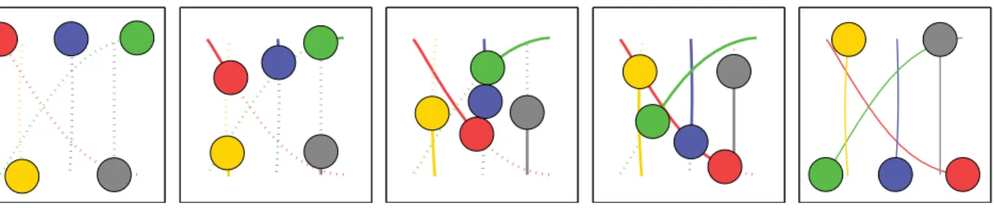
Fig. 2. Collision-free trajectories demonstrated for a 2D scenario. The circles show the positions of the vehicles (and the required minimum distance) in thexy-plane at subsequent times from left to right. The lines indicate the resulting trajectories.
limit values in (12) and (15), so that the resulting trajectory is likely feasible. However, this excludes too many feasible trajectories.
Second, the constraints are satisfied only at discrete times k: The actual trajectories are found by linear interpolation and may, for example, not fulfill the minimum distance re-quirement between discrete times. This issue, can be readily addressed with a smaller time steph. However, this increases the problem dimension.
The solution adopted in this paper is to use an external algorithm to verify the feasibility of the trajectories returned by the SCP. On the one hand, this allows us to abstract the trajectory generation problem, which is thus almost totally independent from the specific vehicle dynamics. On the other hand, the feasibility test is performed on the interpo-lated trajectories, addressing possible constraint violations between discrete times. In the next section, we introduce the overall algorithm and explain how we deal with infeasible trajectories.
IV. THE ALGORITHM
The overall algorithm consists of the following steps:
1: Initialization: Check if initial and final states satisfy the constraints. Select initial values for handT.
2: Solve the SCP, as described in Sec. III. 3: Check the resulting trajectories for feasibility.
If they are feasible, exit. Otherwise, adjust T or h and go back to 2.
A. Initialization
Firstly, the initial and final states must satisfy the con-straints. Secondly, initial values for the discretization time stephand the trajectory durationT are chosen. Our results show that a medium time step h (e.g. h = 0.2s) is often sufficient to fulfill the minimum distance requirement between discrete times, with the advantage of keeping the problem dimension small. The choice of T depends on the desired duration of the transition from the initial set of states to the final one. Keep in mind that a smallTwill more likely violate the vehicle’s physical limits, thus the initial guess must be tailored to the capabilities of the vehicle. Notice that a big value ofT results in a larger problem dimension. In our approach, h and T are modified if the trajectories
resulting from the SCP step are infeasible (see Sec. IV-C). However, an appropriate initial choice will avoid unnecessary iterations (see Sec. V-A.3) and speed up the generation of feasible trajectories.
B. Feasibility check
The discrete trajectories resulting from the SCP step are first linearly interpolated and then checked for feasibility with respect to the vehicle’s physical limits and position constraints.
1) Vehicle’s physical limits: We developed a method that uses a first-principles model of the quadrocopter dynamics, to relate the quadrocopter trajectory to the required rotational rates and rotor forces. These are constrained by actuator and sensor limitations. The algorithm requires a trajectory in the 3D space and a yaw profile. In this paper, we assume a constant yaw angle and use the algorithm presented in [19] for a sophisticated feasibility check.
The method also provides guidelines for designing feasible trajectories for quadrocopters. The main conclusion is that the jerk must be bounded. Intuitively, requiring a bounded jerk implies continuity in the quadrocopter’s attitude. Thus, the constraints of the SCP (acceleration and jerk) allow the algorithm to return a solution that is likely to be feasible.
2) Position constraints: The trajectories resulting from the SCP step are guaranteed to meet position and avoid-ance constraints only at discrete time steps k. Therefore, constraints (10) and (16) are verified for the interpolated trajectories as well.
C. Parameter adaptation
If the trajectories resulting from the SCP step are not feasible because of the vehicle’s physical limits, we increase the trajectory duration time T and recompute the SCP step. This is motivated by the fact that with T → ∞, the input converges to zero and a feasible solution must be found.
Instead, if position constraints are violated between dis-crete times, we decrease hand restart the SCP with a finer resolution. Both adjustments result in a larger problem di-mension.
V. RESULTS
The resulting trajectories are smooth. Fig. 2 shows the evolution of the position of 5 vehicles over time for a 2D case. In the following, we present some results on the
2000 3000 4000 5000 6000 7000 8000 9000 10000 0 2 4 6 8 10 12
Number of inequality constraints M [−]
A ve ra ge c om pu ta tio n tim e [s ]
Fig. 3. The average computation time per SCP iteration as a function of the numberM of inequality constraints (50 trials for each case). The error bars indicate the standard deviation. The grey area indicates the average time needed for the initialization of the algorithm.
computational time and on the application of this method to quadrocopters in the ETH Flying Machine Arena (FMA).
A. Computational effort
We present here some results of the needed computational time. All our experiments were conducted on a PC running Windows 7, and equipped with an Intel Core 2 Duo CPU E8500 @3.16 Ghz and 6 GB of RAM. The next three ex-periments assume that the vehicles must transition between randomly picked positions (with zero initial and final velocity and acceleration) in a 6 x 6 x 6 m space. Minimum distance between vehicles isR= 1m.
1) Computational time: We run the algorithm with differ-ent values forN andK. Fig. 3 shows the average time nec-essary to complete a single SCP iteration for various values of M, which indicate the number of inequality constraints, see (18). We can conclude that the value ofMis a reasonable indication of the time necessary to compute a solution.
A typical operational scenario in the FMA (e.g. a takeoff phase) that involves 5 vehicles performing 3-second long trajectories with h= 0.2s results in M = 2050. The total computation time of feasible trajectories is on average0.31s.
2) Necessary SCP iterations: The total number of SCP iterations necessary for the solutionχq to converge is shown
in Fig. 4. Usually, the algorithm converges in less than 4 iterations. The large deviation depends on the initial configuration of the vehicles, which is randomly picked as explained above. Intuitively, the number is larger if the final trajectories deviate a lot from the ideal straight ones.
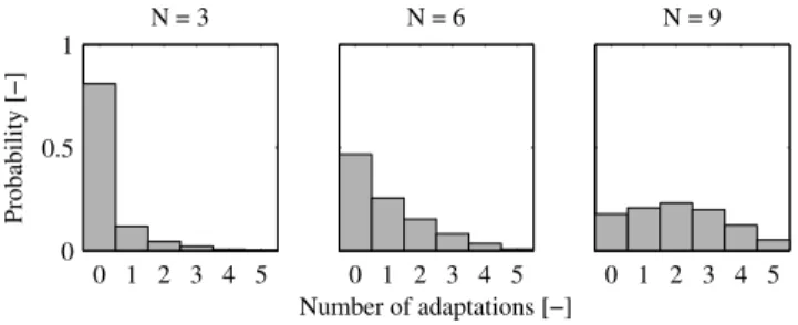
3) Parameter adaptation: The algorithm adapts the pa-rametersT andhif the resulting trajectories are not feasible (see Sec. IV-C). We generated trajectories for different values of N using T = 3s and h= 0.2s as initial values. Fig. 5 shows how often the algorithm needs to adapt the parameters depending on the number of vehicles in the space. It is clear from the results that a good initial guess must take into account the number of vehicles crowding the space.
4 5 6 7 8 9 10 11 12 0 1 2 3 4 Number of vehicles N [−] N um be r o f S C P ite ra tio ns [− ]
Fig. 4. The average number of SCP iterations as a function of the number N of vehicles (800 trials per case). The error bars indicate the standard deviation. 0 1 2 3 4 5 0 0.5 1 N = 3 Pr ob ab ili ty [− ] 0 1 2 3 4 5 N = 6 Number of adaptations [−] 0 1 2 3 4 5 N = 9
Fig. 5. The histograms show the number of adaptations necessary to obtain a feasible solution for different values ofN (probability over 900 tries). Initial values areT= 3s andh= 0.2s.
Intuitively, with many vehicles in the space trajectories are longer, since they have to avoid each other.
B. Experimental testbed
We demonstrate our algorithm on small custom quadro-copters in the Flying Machine Arena, a 10 x 10 x 10 m testbed for quadrocopter research. The space is equipped with a motion capture system that provides precise vehicle position and attitude measurements at high rates. This information is sent to a PC, which runs algorithms and control strategies, and sends commands to the quadrocopter at approximately 60 Hz. More details on the testbed can be found in [20].
C. Online generation of feasible collision-free trajectories
The algorithm is currently used for takeoff and land-ing operation with multiple vehicles in the FMA. The video attached to this submission and available online
(http://youtu.be/wwK7WvvUvlI) demonstrates the
speed of the algorithm. In the first part of the video, the destination points are selected ahead of time and collision-free trajectories are pre-computed. All the trajectories are stored before execution. In the second part of the video, however, the next set of destination points is picked at ran-dom while the vehicles are still en-route, demonstrating that the algorithm is fast enough to be used in real-time. Fig. 6 shows an example of collision-free trajectories generated by
−2 0 2 −2.5 −2 −1.5 −1 −0.5 0 0.5 1 1.5 2 2.5 3 3.5 y [m] x [m] z [m ]
Fig. 6. Collision-free trajectories flown by quadrocopters in the Flying Machine Arena. The triangles indicate the initial points. The squares represent the goal points. It can be seen how the trajectories deviate from the straight paths that would have resulted in collisions.
the algorithm and actually flown in the FMA. The initial and final points are randomly picked.
VI. CONCLUSIONS
The method presented in this paper allows for the gen-eration of collision-free trajectories for multiple vehicles within seconds. This algorithm is currently successfully used in the FMA when working with multiple vehicles. It allows for takeoff and landing from arbitrary locations, safely leading the quadrocopters to the desired points in space. The algorithm is also incorporated into a software tool that allows us to easily generate quadrocopter choreographies for a pre-processed music piece. It enables us to create smooth transition motions between different motion primitives when creating dance performances with quadrocopters [21].
The algorithm is generally independent of the vehicle’s type. However, knowledge about the vehicle influences the choice of the appropriate inequality constraints, and leads to more reliable results. In addition, if linear expressions do not capture vehicle constraints precisely enough, an appropriate vehicle-specific feasibility check is necessary.
Decoupling complex vehicle dynamics and constraints from the trajectory generator simplifies the planning problem and results in a fast and efficient way for generating collision-free trajectories. Planning trajectories while accounting for vehicle constraints is complex. Checking a posteriori if a trajectory satisfies these constraints is fast, and can be done using a complex vehicle model. This paper demonstrates the effectiveness of this approach, when applied to quadro-copters. The approach can be similarly applied to other vehicles and problems.
ACKNOWLEDGMENTS
The authors thank Yang Wang and Stephen Boyd for the introduction to SCP and its possible applications. The authors acknowledge the contributions of the FMA team, in particular Markus Hehn, Sergei Lupashin, and Mark W. Mueller.
REFERENCES
[1] S. Boyd, “Sequential Convex Programming,” Lecture Notes, Stanford University, 2008. [Online]. Available: http://www.stanford.edu/class/ee364b/lectures/seq slides.pdf [2] Y. Wang, E. Akuiyibo, and S. Boyd, “Applications of
convex optimization in control,” Talk, 2011. [Online]. Available: http://www.stanford.edu/∼yw224/eth talk.pdf
[3] M. Hehn and R. D’Andrea, “Quadrocopter Trajectory Generation and Control,” inIFAC World Congress, 2011, pp. 1485–1491.
[4] D. Mellinger and V. Kumar, “Minimum snap trajectory generation and control for quadrotors,” inIEEE International Conference on Robotics and Automation, May 2011, pp. 2520–2525.
[5] A. Richards and J. How, “Aircraft trajectory planning with collision avoidance using mixed integer linear programming,” in American Control Conference, vol. 3, 2002, pp. 1936–1941.
[6] C. Goerzen, Z. Kong, and B. Mettler, “A Survey of Motion Planning Algorithms from the Perspective of Autonomous UAV Guidance,”
Journal of Intelligent and Robotic Systems, vol. 57, no. 1-4, pp. 65– 100, Nov. 2009.
[7] F. Kendoul, “Survey of advances in guidance, navigation, and control of unmanned rotorcraft systems,”Journal of Field Robotics, vol. 29, no. 2, pp. 315–378, Mar. 2012.
[8] R. Siegwart, I. R. Nourbakhsh, and D. Scaramuzza,Introduction to autonomous mobile robots. Cambridge, MA : MIT Press, 2011. [9] J. H. Gillula, G. M. Hoffmann, M. P. Vitus, and C. J. Tomlin,
“Applications of hybrid reachability analysis to robotic aerial vehicles,”
The International Journal of Robotics Research, vol. 30, no. 3, pp. 335–354, Jan. 2011.
[10] Y. Kuwata, A. Richards, T. Schouwenaars, and J. P. How, “Distributed Robust Receding Horizon Control for Multivehicle Guidance,”IEEE Transactions on Control Systems Technology, vol. 15, no. 4, pp. 627– 641, Jul. 2007.
[11] A. U. Raghunathan, V. Gopal, D. Subramanian, L. T. Biegler, and T. Samad, “Dynamic optimization strategies for three-dimensional conflict resolution of multiple aircraft,”Journal of guidance, control, and dynamics, vol. 27, no. 4, pp. 586–594, 2004.
[12] J. Snape, J. van den Berg, S. J. Guy, and D. Manocha, “Smooth and collision-free navigation for multiple robots under differential-drive constraints,” inEEE/RSJ International Conference on Intelligent Robots and Systems, Oct. 2010, pp. 4584–4589.
[13] H. Yuan and Z. Qu, “Optimal real-time collision-free motion planning for autonomous underwater vehicles in a 3D underwater space,”IET Control Theory Applications, vol. 3, no. 6, p. 712, 2009.
[14] T. Schouwenaars, J. How, and E. Feron, “Decentralized cooperative trajectory planning of multiple aircraft with hard safety guarantees,” inProceedings of the AIAA Guidance, Navigation and Control Con-ference, 2004.
[15] B. Varghese, G. McKee, L. Beji, S. Otmane, and A. Abichou, “Towards a Unifying Framework for Pattern Transformation in Swarm Systems,” inAIP Conference Proceedings, vol. 1107, no. 1. AIP, Mar. 2009, pp. 65–70.
[16] J. Alonso-Mora, A. Breitenmoser, M. Rufli, R. Siegwart, and P. Beard-sley, “Multi-robot system for artistic pattern formation,” in IEEE International Conference on Robotics and Automation, May 2011, pp. 4512–4517.
[17] S. Boyd and L. Vandenberghe,Convex Optimization. Cambridge University Press, 2004.
[18] “IBM ILOG CPLEX Optimizer.” [Online]. Avail-able: http://www.ibm.com/software/integration/optimization/cplex-optimizer
[19] F. Augugliaro, “Dancing Quadrocopters - Trajectory Generation, Feasibility and User Interface,” Master’s Thesis, ETH Zurich, 2011. [Online]. Available: http://dx.doi.org/10.3929/ethz-a-007328864 [20] S. Lupashin, A. Schoellig, M. Sherback, and R. D’Andrea, “A simple
learning strategy for high-speed quadrocopter multi-flips,” in IEEE International Conference on Robotics and Automation, May 2010, pp. 1642–1648.
[21] A. Schoellig, F. Augugliaro, S. Lupashin, and R. D’Andrea, “Synchro-nizing the motion of a quadrocopter to music,” inIEEE International Conference on Robotics and Automation, May 2010, pp. 3355–3360.