Bera, A. K., Galvao Jr, A. F., Montes-Rojas, G. & Park, S. Y. (2010). Which quantile is the most informative? Maximum likelihood, maximum entropy and quantile regression (Report No. 10/08).
London, UK: Department of Economics, City University London.
City Research Online
Original citation: Bera, A. K., Galvao Jr, A. F., Montes-Rojas, G. & Park, S. Y. (2010). Which quantile is the most informative? Maximum likelihood, maximum entropy and quantile regression (Report No. 10/08). London, UK: Department of Economics, City University London.
Permanent City Research Online URL: http://openaccess.city.ac.uk/1483/ Copyright & reuse
City University London has developed City Research Online so that its users may access the research outputs of City University London's staff. Copyright © and Moral Rights for this paper are retained by the individual author(s) and/ or other copyright holders. Users may download and/ or print one copy of any article(s) in City Research Online to facilitate their private study or for non-commercial research. Users may not engage in further distribution of the material or use it for any profit-making activities or any commercial gain. All material in City Research Online is checked for eligibility for copyright before being made available in the live archive. URLs from City Research Online may be freely distributed and linked to from other web pages.
Versions of research
The version in City Research Online may differ from the final published version. Users are advised to check the Permanent City Research Online URL above for the status of the paper.
Enquiries
If you have any enquiries about any aspect of City Research Online, or if you wish to make contact with the author(s) of this paper, please email the team at [email protected].
Department of Economics
Which Quantile is the Most Informative?
Maximum Likelihood, Maximum Entropy and
Quantile Regression
Anil K. Bera
University of Illinois, Urbana-Champaign
Antonio F. Galvao Jr.
University of Wisconsin-Milwaukee
Gabriel Montes-Rojas*
City University London
Sung Y. Park
University of Illinois, Urbana-Champaign
Department of Economics Discussion Paper Series
No. 10/08
* Department of Economics, City University London, Social Sciences Bldg, Northampton Square, London EC1V 0HB, UK.
Which Quantile is the Most Informative? Maximum
Likelihood, Maximum Entropy and Quantile Regression
∗
Anil K. Bera
†Antonio F. Galvao Jr.
‡Gabriel V. Montes-Rojas
§Sung Y. Park
¶Abstract
This paper studies the connections among quantile regression, the asymmetric Laplace distribution, maximum likelihood and maximum entropy. We show that the maximum likeli-hood problem is equivalent to the solution of a maximum entropy problem where we impose moment constraints given by the joint consideration of the mean and median. Using the resulting score functions we propose an estimator based on the joint estimating equations. This approach delivers estimates for the slope parameters together with the associated “most probable” quantile. Similarly, this method can be seen as a penalized quantile regression estimator, where the penalty is given by deviations from the median regression. We derive the asymptotic properties of this estimator by showing consistency and asymptotic normal-ity under certain regularnormal-ity conditions. Finally, we illustrate the use of the estimator with a simple application to the U.S. wage data to evaluate the effect of training on wages.
Keywords: Quantile Regression; Treatment Effects; Asymmetric Laplace Distribution
JEL classification: C14; C31
∗We are very grateful to Arnold Zellner, Jushan Bai, Rong Chen, Daniel Gervini, Yongmiao Hong, Carlos
Lamarche, Ehsan Soofi, Zhijie Xiao, and the participants in seminars at University of Wisconsin-Milwaukee, City University London, World Congress of the Econometric Society, Shanghai, August 2010, Latin American Meeting of the Econometric Society, Argentina, October 2009, Summer Workshop in Econometrics, Tsinghua University, Beijing, China, May 2009, South Asian and Far Eastern Meeting of the Econometrics Society, Singapore, July 2008, for helpful comments and discussions. However, we retain the responsibility for any remaining errors.
†Department of Economics, University of Illinois, 1407 W. Gregory Drive, Urbana, IL 61801. Tel.:
+1-217-3334596; fax: +1-217-2446678. E-mail: [email protected]
‡Department of Economics, University of Wisconsin-Milwaukee, Bolton Hall 852, 3210 N. Maryland Ave.,
Milwaukee, WI 53201. E-mail: [email protected]
§Department of Economics, City University of London, 10 Northampton Square, London EC1V 0HB,
U.K. E-mail: [email protected]
¶Department of Economics, University of Illinois, 1407 W. Gregory Drive, Urbana, IL 61801, and The
Wang Yanan Institute for Studies in Economics, Xiamen University, Xiamen, Fujian 361005, China. E-mail:
1
Introduction
Different choices of loss functions determine different ways of defining the location of a random variable y. For example, squared, absolute value, and step function lead to mean, median and mode, respectively (see Manski, 1991, for a general discussion). For a given quantile τ ∈(0,1), consider the loss function in a standard quantile estimation problem,
L1,n(µ;τ) = n X i=1 ρτ(yi−µ) = n X i=1 (yi−µ) (τ−1(yi ≤µ)), (1)
as proposed by Koenker and Bassett (1978). Minimizing L1,n with respect to the location
parameter µ is identical to maximizing the likelihood based on the asymmetric Laplace probability density (ALPD):
f(y;µ, τ, σ) = τ(1−τ) σ exp −ρτ(yσ−µ) , (2)
for givenτ. The well known symmetric Laplace (double exponential) distribution is a special case of (2) when τ=1/2.
Several studies developed the properties of the maximum likelihood (ML) estimators based on ALPD. Hinkley and Revankar (1977) derived the asymptotic properties of the unconditional MLE under ALPD. Kotz, Kozubowski, and Podg´orsk (2002b) and Yu and Zhang (2005) consider alternative MLE approaches for ALPD. Moreover, models based on ALPD have been proposed in different contexts. Machado (1993) used the ALPD to derive a Schwartz information crietrion for model selection for quantile regression (QR) models, and Koenker and Machado (1999) introduced a goodness-of-fit measure for QR and related inference processes. Yu and Moyeed (2001) and Geraci and Botai (2007) used a Bayesian QR approach based on the ALPD. Komunjer (2005) constructed a new class of estimators for conditional quantiles in possibly misspecified nonlinear models with time series data. The proposed estimators belong to the family of quasi-maximum likelihood estimators (QMLEs) and are based on a family of ‘tick-exponential’ densities. Under the asymmetric Laplace density, the corresponding QMLE reduces to the Koenker and Bassett (1978) linear quantile regression estimator. In addition, Komunjer (2007) developed a parametric estimator for the
risk of financial time series expected shortfall based on the asymmetric power distribution, derived the asymptotic distribution of the maximum likelihood estimator, and constructed a consistent estimator for its asymptotic covariance matrix.
Interestingly, the parameter µ in functions (1) and (2) is at the same time the location parameter, the τ-th quantile, and the mode of the ALPD. For the simple (unconditional) case, the minimization of (1) returns different order-statistics. For example, if we set τ =
{0.1,0.2, ...,0.9}, the solutions are, respectively, the nine deciles of y. In order to extract important information from the data a good summary statistic would be to chooseone order statistics accordingly the most likely value. For a symmetric distribution one would choose the median. Using the ALPD, for given τ, maximization of the corresponding likelihood function gives that particular order statistics. Thus, the main idea of this paper is to jointly
estimate τ and the corresponding order statistic ofywhich can be taken as a good summary statistic of the data. The above notion can be easily extended to modeling the “conditional location” of y given covariates x, as we do in Section 2.3. In this case, the ALPD model provides a twist to the QR problem, as nowτ becomes themost likely quantilein a regression set-up.
The aim of this paper is threefold. First, we show that the score functions implied by the ALPD-ML estimation are not restricted to the true data generating process being ALPD, but they arise as the solution to a maximum entropy (ME) problem where we impose moment constraints given by the joint consideration of the mean and median. By so doing, the ALPD-ML estimator combines the information in the mean and the median to capture the asymmetry of the underlying empirical distribution (see Park and Bera, 2009, for a related discussion).
Secondly, we propose a novel Z-estimator that is based on the estimating equations from the MLE score functions (which also correspond to the ME problem). We refer to this esti-mator as ZQR. The approximate Z-estiesti-mator do not impose that the underline distribution is ALPD. Thus, although the original motivation for using the estimating equations is based on the ALPD, the final estimator is independent of this requirement. We derive the asymptotic properties of the estimator by showing consistency and asymptotic normality under certain
regularity conditions. This approach delivers estimates for the slope parameters together with the associated ‘most probable’ quantile. The intuition behind this estimator works as follows. For the symmetric and unimodal case the selected quantile is the median, which coincides with the mean and mode. On the other hand, when the mean is larger than the median, the distribution is right skewed. Thus, taking into consideration the empirical distri-bution, there is more probability mass to the left of the distribution. As a result it is natural to consider a point estimate in a place with more probability mass. The selected τ-quantile does not necessarily lead to the mode, but to a point estimate that is most probable. This provides a new interpretation of QR and frames it within the ML and ME paradigm.
The proposed estimator has an interesting interpretation from a policy perspective. The QR analysis gives a full range of estimators that account for heterogeneity in the response variable to certain covariates. However, the proposed ZQR estimator answers the question: of all the heterogeneity in the conditional regression model, which one is more likely to be observed? In general, the entire QR process is of interest because we would like to either test global hypotheses about conditional distributions or make comparisons across different quantiles (for a discussion about inference in QR models see Koenker and Xiao, 2002). But selecting a particular quantile provides an estimator as parsimonious as ordinary least squares (OLS) or the median estimators. The proposed estimator is, therefore, a complement to the QR analysis rather than a competing alternative. This set-up also allows for an alternative interpretation of the QR analysis. Consider, for instance, the standard conditional regression set-up,y =x′β+u, and letβ be partitioned intoβ = (β
1, β2). For a given value ofβ1 = ¯β1,
we may be interested in finding the representative quantile of the unobservables distribution that corresponds to this level of β1. For such a case, instead of assuming a given quantile
τ we would like to estimate it. In other words, the QR process provides us with the graph β1(τ), but the graph τ(β1) could be of interest too.
Finally, thethird objective of this work is to illustrate the implementation of the proposed ZQR estimator. We apply the estimator to the estimation of quantile treatment effects of subsidized training on wages under the Job Training Partnership Act (JTPA). We discuss the relationship between OLS, median regression and ZQR estimates of the JTPA treatment
effect. We show that each estimator provides different treatment effect estimates. More-over, we extend our ZQR estimator to Chernozhukov and Hansen (2006, 2008) instrumental variables strategy in QR.
The rest of the paper is organized as follows. Section 2 develops the ML and ME frame-works of the problem. Section 3 derives the asymptotic distribution of the estimators. In Section 4 we report a small Monte Carlo study to assess the finite sample performance of the estimator. Section 5 deals with an empirical illustration to the effect of training on wages. Finally, conclusions are in the last section.
2
Maximum Likelihood and Maximum Entropy
In this section we describe the MLE problem based on the ALPD and show its connection with the maximum entropy. We show that they are equivalent under some conditions. In the next section we will propose an Z-estimator based on the resulting estimating equations from the MLE problem, which corresponds to ME.
2.1
Maximum Likelihood
Using (2), consider the maximization of the log-likelihood function of an ALPD: L2,n(µ, τ, σ) =nln 1 στ(1−τ) − n X i=1 1 σρτ(yi−µ) =nln 1 στ(1−τ) −σ1L1,n(µ;τ), (3)
with respect toµ,τ andσ. The first order conditions from (3) lead to the following estimating equations (EE): n X i=1 1 σ 1 2sign(yi −µ) +τ− 1 2 = 0, (4) n X i=1 1−2τ τ(1−τ) − (yi−µ) σ = 0, (5) n X i=1 −σ1 + 1 σ2ρτ(yi−µ) = 0. (6)
Let (ˆµ,τ ,ˆ σ) denote the solution to this system of equations. The first equation leads toˆ the most probable order statistic. Once we have ˆτ, (1−2ˆτ) will provide a measure of asym-metry of the distribution. Equation (6) provides a straightforward measure of dispersion, namely, ˆ σ = 1 n n X i=1 ρτˆ(yi−µ).ˆ
Then, the loss function corresponding to (3) can be rewritten as a two-parameter loss function −1 nL2,n(µ, τ) = ln 1 nL1,n(µ;τ) −ln (τ(1−τ)). (7) This determines that L2,n(µ, τ, σ) can be seen as a penalized quantile optimization function,
where we minimize ln 1
nL1,n(µ;τ)
and penalize it by −ln (τ(1−τ)). The penalty can be interpreted as the cost of deviating from the median, i.e. for τ = 1/2, −ln (τ(1−τ)) =
−ln(1/4) is the minimum, while for either τ →0 or τ →1 the penalty goes to +∞.
It is important to note that the structure of the estimating functions suggests that the solution to the MLE problem can be obtained by first obtaining every quantile of the dis-tribution, and then plugging them (with the corresponding estimator forσ) in (5) until this equation is satisfied (if the solution is unique). In other words, given all the quantiles of y, the problem above selects the most likely quantile as if the distribution of y were ALPD.
2.2
Maximum Entropy
The ALPD can be characterized as a maximum entropy density obtained by maximizing Shannon’s entropy measure subject to two moment constraints (see Kotz, Kozubowski, and Podg´orsk, 2002a):
fM E(y)≡arg max f − Z f(y) lnf(y)dy (8) subject to E|y−µ| = c1, (9) E(y−µ) = c2, (10)
and the normalization constraint, R f(y)dy = 1, where c1 and c2 are known constants. The
solution to the above optimization problem using the Lagrangian has the familiar exponential form
fM E(y:µ, λ1, λ2) =
1
Ω(θ)exp [−λ1|y−µ| −λ2(y−µ)], −∞< y < ∞, (11) whereλ1 and λ2 are the Lagrange multipliers corresponding to the constraints (9) and (10),
respectively, θ = (µ, λ1, λ2)′ and Ω(θ) is the normalizing constant. Note that λ1 ∈ R+ and
λ2 ∈ [−λ1, λ1] so that fM E(y) is well-defined. Symmetric Laplace density (LD) is a special
case of ALPD when λ2 is equal to zero.
Interestingly, the constraints (9) and (10) capture, respectively, the dispersion and asym-metry of the ALPD. The marginal contribution of (10) is measured by the Lagrangian multiplier λ2. If λ2 is close to 0, then (10) does not have useful information for the data,
and therefore, the symmetric LD is the most appropriate. In this case, µis known to be the median of the distribution. On the other hand, when λ2 is not close to zero, it measures the
degree of asymmetry of the ME distribution. Thus the non-zero value of λ2 makes fM E(·)
deviate from the symmetric LD, and therefore, changes the location, µ, of the distribution to adhere the maximum value of the entropy (for general notion of entropy see Soofi and Retzer, 2002).
Let us write (9) and (10), respectively, as
Z
φ1(y, µ)fM E(y:µ, λ1, λ2)dy= 0 and
Z
φ2(y, µ)fM E(y:µ, λ1, λ2)dy= 0,
where φ1(y, µ) = |y−µ| −c1 and φ2(y, µ) = (y−µ)−c2. By substituting the solution
fM E(y : µ, λ1, λ2) into the Lagrangian of the maximization problem in (8), we obtain the
profiled objective function
h(λ1, λ2, µ) = ln Z exp " − 2 X j=1 λjφj(y, µ) # dy. (12)
The parametersλ1,λ2 andµcan be estimated by solving the following saddle point problem
(Kitamura and Stutzer, 1997) ˆ µM E = arg max µ ln Z exp " − 2 X j=1 ˆ λj,M Eφj(y, µ) # dy, where ˆλM E = (ˆλ1,M E,λˆ2,M E) is given by ˆ λM E(µ) = arg min λ ln Z exp " − 2 X j=1 λjφj(y, µ) # dy.
Solving the above saddle point problem is relatively easy since the profiled objective function has the exponential form. However, generally, c1 and c2 are not known or functions of
parameters and Lagrange multipliers in a non-linear fashion. Moreover, in some cases, the closed form of c1 and c2 is not known. In order to deal with this problem, we simply
consider the sample counterpart of the moments c1 and c2, say, c1 = (1/n)Pni=1|yi −µ|
and c2 = (1/n)Pni=1(yi −µ). Then, it can be easily shown that the profiled objective
function is simply the negative log-likelihood function of asymmetric Laplace density, i.e., h(λ1, λ2, µ) =−(1/n)L2,n(µ, τ, σ) (see Ebrahimi, Soofi, and Soyer, 2008). In this case, ˆµM E
and ˆλM E satisfy the following first order conditions∂h/∂µ= 0,∂h/∂λ2 = 0 and∂h/∂λ1 = 0,
respectively: −λn1 n X i=1 sign(yi−µ)−λ2 = 0. (13) 2λ2 (λ1+λ2)(λ1−λ2) + 1 n n X i=1 (yi−µ) = 0, (14) −λ1 1 λ2 1+λ22 λ2 1−λ22 + 1 n n X i=1 |yi−µ|= 0, (15)
Equations (13)-(15) are a re-parameterized version of (4)-(6). In fact, from a comparison of (2) and (11) we can easily see thatλ1 = 1/(2σ),λ2 = (2τ−1)/(2σ) and Ω(θ) =σ/(τ(1−τ)).
Given λ1 the degree of asymmetry is explained by λ2 that is proportionally equal to 2τ−1
in ALPD. Note that λ2 = 0 when τ = 0.5, i.e., µ is the median. Thus finding the most
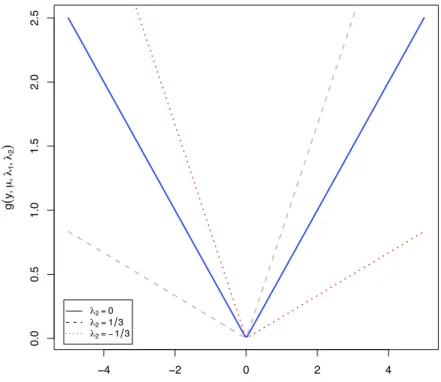
The role of the two moment constraints can be explained by the linear combination of two moment functions, |y−µ|and (y−µ). Figure 1 plotsg(y;λ1, λ2, µ) = λ1|y−µ|+λ2(y−µ)
with three different values ofλ2, λ1 = 1, andµ= 0. In general,g(y;λ1, λ2, µ) can be seen as
a loss function. Clearly, this loss function is symmetric when λ2 = 0. When λ2 = 1/3, g(·)
is tilted so that it puts more weight on the positive values in order to attain the maximum of the Shannon’s entropy (and the reverse is true for λ2 =−1/3). This naturally yields the
asymmetric behavior of the resulting ME density.
[Figure 1]
2.3
Linear Regression Model
Now consider the conditional version of the above, by taking a linear model of the form y =x′β+u, where the parameter of interest is β ∈Rp, x refers to a p-vector of exogenous
covariates, and u denotes the unobservable component in the linear model. As noted in Angrist, Chernozhukov, and Fern´andez-Val (2006), QR provides the best linear predictor for y under the asymmetric loss function
L3,n(β;τ) = n X i=1 ρτ(yi−x′iβ) = n X i=1 ((yi −x′iβ) (τ −1(yi ≤x′iβ))), (16)
whereβ is assumed to be a function of the fixed quantile τ of the unobservable components, that is β(τ). If u is assumed to follow an ALPD, the log-likelihood function is
L4,n(β, τ, σ) = nln 1 στ(1−τ) − n X i=1 1 σρτ(yi−x ′ iβ) = nln 1 στ(1−τ) − 1 σL3,n(β;τ). (17) Estimating β in this framework provides the marginal effect ofx on theτ-quantile of the conditional quantile function of y.
Computationally, the MLE can be obtained by simulating a grid of quantiles and choosing the quantile that maximizes (17), or by solving the estimating equations,∇L4,n(β, τ, σ) = 0,
i.e., ∂L4,n(β, τ, σ) ∂β = n X i=1 1 σ 1 2sign(yi−x ′ iβ) +τ− 1 2 xi = 0, (18) ∂L4,n(β, τ, σ) ∂τ = n X i=1 1−2τ τ(1−τ) − (yi−x′iβ) σ = 0, (19) ∂L4,n(β, τ, σ) ∂σ = n X i=1 −σ1 + 1 σ2ρτ(yi−x′iβ) = 0. (20)
As we stated before, L4,n can be written as a penalized QR problem loss function that
depends only on (β, τ): −n1L4,n(β, τ) = ln 1 nL3,n(β;τ) −ln (τ(1−τ)), (21) and the interpretation is the same as discussed in section 2.1.
3
A Z-estimator for Quantile Regression
In this section we propose a Z-estimator based on the score functions from equations (18)-(20). Thus, although the original motivation for using the estimating equations is based on the ALPD, the final estimator is independent of this requirement. Let k · kbe the Euclidean norm and θ = (β, τ, σ)′. Moreover, define the estimating functions
ψθ(y, x) = ψψ12θθ(y, x)(y, x) ψ3θ(y, x) = 1 σ(τ−1(y < x′β))x 1−2τ τ(1−τ) − (y−x′β) σ −σ1 + 1 σ2ρτ(y−x′β) , and the estimating equations
Ψn(θ) = 1 n n X i=1 1 σ (τ−1(yi < x′iβ))xi 1−2τ τ(1−τ) − (yi−x′iβ) σ −1σ + 1 σ2ρτ(yi−x′iβ) = 1 n n X i=1 ψθ(yi, xi) = 0.
A Z-estimator ˆθn is the approximate zero of the above data-dependent function that
satisfies kΨn(ˆθn)k p
The implementation of the estimator is simple. As discussed in the previous section, an iteration algorithm can be used to solve for the estimates in the estimating equations above. Computationally, the estimates can be obtained by constructing a grid for quantiles τ and solving the QR problem as in (18) and (19) to find ˆβ(τ) and ˆσ(τ). Finally, we estimate the quantile ˆτ that finds an approximate zero in (20). This algorithm is similar to the one proposed in Hinkley and Revankar (1977) and Yu and Zhang (2005) that compute the estimators for MLE under the ALPD. We find that the algorithm converges fast and is very precise.
In the proposed Z-estimator the interpretation of the parameter β is analogous to the interpretation of the location parameter in the QR literature. As in the least squares case, the scale parameter σ can be interpreted as the expected value of the loss function, which in the QR case corresponds to the expectation of the ρτ(.) function. Finally, τ captures a
measure of asymmetry of the underline distribution of y|x and also is associated with the most probable quantile. In the Appendix A we discuss the interpretation of these parameters in more detail.
We introduce the following assumptions to derive the asymptotic properties.
Assumption 1. Let yi = x′iβ0 +ui, i = 1,2, ..., n, where (yi, xi) is independent and
identically distributed (i.i.d.), andxi is independent of ui,∀i.
Assumption 2. The conditional distribution function of y,G(y|x), is absolutely
contin-uous with conditional densities, g(y|x), with 0< g(·|·)<∞.
Assumption 3. Let Θ be a compact set, with θ = (β, τ, σ)′ ∈ Θ, where β ∈ B ⊂ Rp,
τ ∈ T ⊂(0,1), and σ∈ S ⊂R+;
Assumption 4. Ekxk2+ǫ <∞, andEkyk2+ǫ <∞ for some ǫ >0.
Assumption 5. (i) Define Ψ(θ) = E[ψθ(y, x)]. Assume that Ψ(θ0) = 0 for a unique
θ0 ∈ intΘ. (ii) Define Ψn(θ) = En[ψθ(y, x)] = 1nPni=1ψθ(yi, xi). Assume that kΨn(ˆθn)k =
op(n−1/2).
Assumption A2 is common in the QR literature and restricts the conditional distribution of the dependent variable. Assumption A3 imposes compactness of the parameter space, and A4 is important to guarantee the asymptotic behavior of the estimator. The first part of A4 is usual in QR literature and second part in least squares literature. Finally Assumption A5 imposes an identifiability condition and ensure that the solution to the estimating equations is “nearly-zero”, and it deserves further discussion.
The first part of A5 imposes a unique solution condition. Similar restrictions are fre-quently used in the QR literature to satisfy E[ψ1θ(y, x)] = 0 for a unique β and any given
τ. This condition also appears in the M and Z estimators literatures. Uniqueness in QR is a very delicate subject and is actually imposed. For instance, Chernozhukov, Fern´andez-Val, and Melly (2009, p. 49) propose an approximate Z-estimator for QR process and assume that the true parameter β0(τ) solves E[(τ −1{y ≤ X′β0(τ)})X] = 0. Angrist,
Chernozhukov, and Fern´andez-Val (2006) impose a uniqueness assumption of the form: β(τ) = arg minβE[ρτ(y −x′β)] is unique (see for instance their Theorems 1 and 2). See
also He and Shao (2000) and Schennach (2008) for related discussion.
It is possible to impose more primitive conditions to ensure uniqueness. These conditions are explored and discussed in Theorem 2.1 in Koenker (2005, p. 36). If the y’s have a bounded density with respect to Lebesgue measure then the observations (y, x) will be in general position with probability one and a solution exists.1 However, uniqueness cannot be
ensured if the covariates are discrete (e.g. dummy variables). If the x’s have a component that have a density with respect to a Lebesgue measure, then multiple optimal solutions occur with probability zero and the solution is unique. However, these conditions are not very attractive, and uniqueness is in general imposed as an assumption.
Note that the usual assumptions of uniqueness in QR described above forE[ψ1θ(y, x)] = 0
guarantee that β is unique for any given τ. Combining these assumptions and bounded moments we guarantee uniqueness forE[ψ3θ(y, x)] = 0, because σ=E[ρτ(y−xβ)] such that
for each τ, σ is unique. With respect to the second equation E[ψ2θ(y, x)] = 0, it is satisfied
if
1−2τ τ(1−τ) =
E[y−x′β]
σ .
Therefore, for unique β and σ, the right hand side of the above equation is unique. Since
1−2τ
τ(1−τ) is a continuous and strictly decreasing, τ is also unique.2
The second part of A5 is used to ensure that the solution to the approximated working estimating equations is close to zero. The solution for the estimating equations, Ψn(ˆθn) = 0,
does not hold in general. In most cases, this condition is actually equal to zero, but least absolute deviation of linear regression is one important exception. The indicator function in the first estimating equations determines that it may not have an exact zero. It is common in the literature to work with M and Z estimators ˆθnof θ0 that satisfyPni=1ψ(xi,θˆn) = op(δn),
for some sequence δn. For example, Huber (1967) considered δn = √n for asymptotic
normality, and Hinkley and Revankar (1977) verified the condition for the unconditional asymmetric double exponential case. This condition also appears in the quantile regression literature, see for instance He and Shao (1996) and Wei and Carroll (2009). In addition, in the approximate Z-estimator for quantile process in Chernozhukov, Fern´andez-Val, and Melly (2009), they have that the empirical moment functions ˆΨ(θ, u) = En[g(Wi, θ, u)], for each
u∈T, the estimator ˆθ(u) satisfieskΨ(ˆˆ θ(u), u)k ≤infθ∈ΘkΨ(θ, u)ˆ k+ǫnwhere ǫn=o(n−1/2).
For the quantile regression case, Koenker (2005, p. 36) comments that the absence of a zero to the problem Ψ1n( ˆβn(τ)) = 0, where ˆβn(τ) is the quantile regression optimal solution
for a given τ and σ, “is unusual, unless the yi’s are discrete.” Here we follow the standard
conditions for M and Z estimators and impose A5(ii). For a more general discussion about this condition on M and Z estimators see e.g. Kosorok (2008, pp. 399-407).
Now we move our attention to the asymptotic properties of the estimator.
Theorem 1 Under Assumptions A1-A5, kθˆn−θ0k
p
→0.
Proof: In order to show consistency we check the conditions of Theorem 5.9 in van der
2Note that m(τ) ≡ 1−2τ
τ(1−τ) is a continuous function, has a unique zero at τ = 1/2 and m(τ) > 0 for
τ < 1/2, m(τ) < 0 for τ > 1/2. As τ → 0, m(τ) → +∞, and as τ → 1, m(τ) → −∞. Finally,
dm(τ) dτ = −2τ(1−τ)−(1−2τ) 2 τ2 (1−τ) 2 = −2 τ+2τ2 −1+4τ−4τ 2 τ2 (1−τ) 2 = −1+2 τ −2τ 2 τ2 (1−τ) 2 =− 1+2τ(1−τ) τ2 (1−τ) 2 <0 for anyτ∈(0,1).
Vaart (1998). Define F ≡ {ψθ(y, x), θ ∈ Θ}, and recall that Ψn(θ) = n1Pni=1ψθ(y, x) and
Ψ(θ) = E[ψθ(y, x)]. First note that, under conditions A3 and A5, the function Ψ(θ) satisfies,
inf
θ:d(θ,θ0)≥ǫk
Ψ(θ)k>0 =kΨ(θ0)k,
because for a compact set Θ and a continuous function Ψ, uniqueness of θ0 as a zero implies
this condition (see van der Vaart, 1998, p.46).
Now we need to show that supθ∈ΘkΨn(θ)−Ψ(θ)k p
→0. By Lemma A1 in the Appendix B we know that the class F is Donsker. Donskerness implies a uniform law of large numbers such that
sup
θ∈Θ|
En[ψθ(y, x)]−E[ψθ(y, x)]|→p 0,
where f 7→En[f(w)] = 1
n Pn
i=1f(wi). Hence we have supθ∈ΘkΨn(θ)−Ψ(θ)k p
→0.
Finally, from assumptions A1-A5 the problem has a unique root and also we have
kΨn(ˆθn)k
p
→0. Thus, all the conditions in Theorem 5.9 of van der Vaart (1998) are satisfied and kθˆn−θ0k
p
→0.
After showing consistency we move our attention to the asymptotic normality of the estimator. In order to derive the limiting distribution define
V1θ =E[ψθ(y, x)ψθ(y, x)′], (22) V2θ = ∂E[ψθ(y, x)] ∂θ′ . (23) Here, V1θ = 1 στ(1−τ)E[xx′] E[((1−2τ)sign(y−x′β)−(1−2τ)2 )x′] 2στ(1−τ) −E h 1 σ2ρτ(y−x′β)x′ i 1 2σ3E[ρτ(y−x′β) (sign(y−x′β)−(1−2τ))x′] . (1−2τ)2 τ2(1 −τ)2 +E[1 σ2(y−x′β)2]−2 (1−2τ) τ(1−τ)E[ 1 σ(y−x′β)] 1 σ2E[ρτ(y−x′β) ((1τ(1−−2ττ))−σ1(y−x′β))] . . σ14E[ρτ2(y−x′β)] + 1 σ2− 1 σ3E[ρτ(y−x′β)] and V2θ = −E[g(x′βσ|x)xx′] 1 σE[x] 0 . −τ1+22(1−τ−τ2)2τ2 σ12E[(y−x′β)] . . −σ12 .
Note that when y|x∼ALP D(x′β, τ, σ), then V
1θ =V2θ.
Assumption 6. Assume that V1θ0 and V2θ0 exist and are finite, and V2θ0 is invertible.
Chernozhukov, Fern´andez-Val, and Melly (2009) calculated equations (22) and (23) in the quantile process as an approximate Z-estimator.
Now we state the asymptotic normality result.
Theorem 2 Under Assumptions 1-6,
√
n(ˆθn−θ0)⇒N(0, V2−θ01V1θ0V−
1 2θ0).
Proof: First, combining Theorem 1 and second part of Lemma A1, we have
Gnψˆ θn(y, x) =Gnψθ0(y, x) +op(1), where f 7→Gn[f(w)] = √1 n Pn i=1(f(wi)−Ef(wi)). Rewriting we have √ nEnψˆ θn(y, x) = √
nEψθˆn(y, x) +Gnψθ0(y, x) +op(1). (24)
By assumption A5
Enψˆ
θn(y, x)
=op(n−1/2) and E[ψθ0(y, x)] = 0.
Now consider the first element of the right hand side of (24). By a Taylor expansion about ˆ
θn =θ0 we obtain
E[ψθˆn(y, x)] = E[ψθ0(y, x)] +
∂E[ψθ(y, x)] ∂θ′ θ=θ0(ˆθn−θ0) +op(1), (25) where ∂E[ψθ(y, x)] ∂θ′ θ=θ0 = ∂ ∂θ′E 1 σ(τ−1(y < x′β))x 1−2τ τ(1−τ) − (y−x′β) σ −σ1 + 1 σ2ρτ(y−x′β) θ=θ0 .
Since by condition A6, ∂E[ψθ(y,x)]
∂θ′
θ=θ0
=V2θ0, equation (25) can be rewritten as
E[ψθ(y, x)]
Using Assumption A5 (ii), from (24) we have
op(1) =√nEψθˆn(y, x) +Gnψθ0(y, x) +op(1),
and using the above approximation given in (26) op(1) =V2θ0 √ n(ˆθn−θ0) +Gnψθ0(y, x) +op(1). By invertibility of V2θ0 in A6, √ n(ˆθn−θ0) = −V2−θ01Gnψθ0(y, x) +op(1). (27)
Finally, from Lemma A1θ 7→Gnψθ(y, x) is stochastic equicontinuous. So, stochastic
equicon-tinuity and ordinary CLT imply thatGnψθ(y, x)⇒z(·) converges to a Gaussian process with
variance-covariance function defined by V1θ0 =E[ψθ(y, x)ψθ(y, x)′] θ=θ0 . Therefore, from (27) √ n(ˆθn−θ0)⇒V2−θ01z(·), so that √ n(ˆθn−θ0)⇒N(0, V2−θ01V1θ0V− 1 2θ0).
4
Monte Carlo Simulations
In this section we provide a glimpse into the finite sample behavior of the proposed ZQR estimator. Two simple versions of our basic model are considered in the simulation experi-ments. In the first, reported in Table 1, the scalar covariate, xi, exerts a pure location shift
effect. In the second, reported in Table 2, xi has both a location and scale shift effects. In
the former case the response, yi, is generated by the model,
while in the latter case,
yi =α+βxi+ (1 +γ)ui,
where ui are i.i.d. innovations generated according to a standard normal distribution, t3
distribution, χ2
3 centered at the mean, Laplace distribution (i.e. τ = 0.5), and ALPD with
τ = 0.25.3 In the location shift model x
i follows a standard normal distribution; in the
location-scale shift model, it follows a χ2
3. We setα =β = 1 and γ = 0.5. Our interest is on
the effect of the covariates in terms of bias and root mean squared error (RMSE). We carry out all the experiments with sample size n = 200 and 5,000 replications. Three estimators are considered: our proposed ZQR estimator, quantile regression at the median (QR), and ordinary least squares (OLS). We pay special attention to the estimated quantile ˆτ in the ZQR.
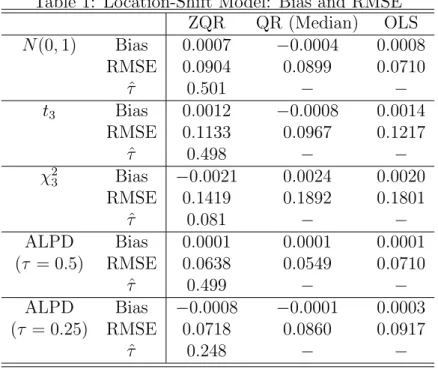
Table 1 reports the results for the location shift model. In all cases we compute the bias and RMSE with respect to β = 1. Bias is close to zero in all cases. In the Gaussian setting, as expected, we observe efficiency loss in ZQR and QR estimates compared to that of OLS. Under symmetric distributions, normal, t3, and Laplace, the estimated quantile of
interest ˆτ in the ZQR is remarkably close to 0.5. In theχ2
3 case, the ZQR estimator performs
better than the QR and OLS procedures. Note that the estimated quantile for the χ2 3 is
0.081, consistent with the fact that the underline distribution is right skewed. Finally, for the ALPD(0.25) case, ZQR produces the estimated quantile (ˆτ = 0.248) rightly close to 0.25, and also has a smaller RMSE. Overall, Table 1 shows that the ZQR estimator retains the robustness properties of the QR estimator, although we do not specify a particular quantile of interest.
[Table 1]
In the location-scale version of the model we adopt the same distributions for generating the data. For this case the effect of the covariatexi on quantile of interest response in QR is
given byβ(τ) =β+γQu(τ). In ZQR we compute bias and RMSE by averaging estimatedτ
from 5,000 replications. The results are summarized in Table 2. The results for the normal,
t3 and Laplace distributions are similar to those in the location model, showing that all point
estimates are approximately unbiased. As expected, OLS outperforms ZQR and QR in the normal case, but the opposite occurs in thet3 and Laplace distributions. In theχ23 case, the
estimated quantile is ˆτ = 0.086. For the ALPD(0.25) distribution, the best performance is obtained for the ZQR estimator.
[Table 2]
5
Empirical Illustration: The Effect of Job Training on
Wages
The effect of policy variables on distributional outcomes are of fundamental interest in em-pirical economics. Of particular interest is the estimation of the quantile treatment effects (QTE), that is, the effect of some policy variable of interest on the different quantiles of a conditional response variable. Our proposed estimator complements the QTE analysis by providing a parsimonious estimator at the most probable quantile value.
We apply the estimator to the study of the effect of public-sponsored training programs. As argued in LaLonde (1995), public programs of training and employment are designed to improve participant’s productive skills, which in turn would affect their earnings and de-pendency on social welfare benefits. We use the Job Training Partnership Act (JTPA), a public training program that has been extensively studied in the literature. For example, see Bloom, Orr, Bell, Cave, Doolittle, Lin, and Bos (1997) for a description, and Abadie, Angrist, and Imbens (2002) for QTE analysis. The JTPA was a large publicly-funded train-ing program that began fundtrain-ing in October 1983 and continued until late 1990’s. We focus on the Title II subprogram, which was offered only to individuals with “barriers to em-ployment” (long-term use of welfare, being a high-school drop-out, 15 or more recent weeks of unemployment, limited English proficiency, phsysical or mental disability, reading pro-ficiency below 7th grade level or an arrest record). Individuals in the randomly assigned JTPA treatment group were offered training, while those in the control group were excluded
for a period of 18 months. Our interest lies in measuring the effect of a training offer and actual training on of participants’ future earnings.
We use the database in Abadie, Angrist, and Imbens (2002) that contains information about adult male and female JTPA participants and non-participants. Let z denote the indicator variable for those receiving a JTPA offer. Of those offered, 60% did training; of those in the control group, less than 2% did training. For our purposes of illustrating the use of ZQR, we first study the effect of receiving a JTPA offer on log wages, and later we pursue instrumental variables estimation in the ZQR context. Following Abadie, Angrist, and Imbens (2002) we use a linear regression specification model, where the JTPA offer enters in the equation as a dummy variable.4 We consider the following regression model:
y=zγ+xβ+u,
where the dependent variable y is the logarithm of 30 month accumulated earnings (we exclude individuals without earnings), z is a dummy variable for the JTPA offer, x is a set of exogenous covariates contaning individual characteristics, and u is an unobservable component. The parameter of interest is γ that provides the effect of the JTPA training offer on wages.
[Table 3 and Figures 2, and 3]
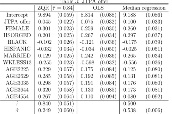
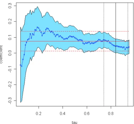
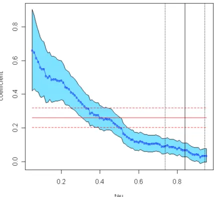
First, we compute the QR process for allτ ∈(0.05,0.95) and the results are presented in Figure 2. The JTPA effect estimates for QR and OLS appear in Table 3. Interestingly, with exception of low quantiles, the effect of JTPA is decreasing in τ, which implies that those individuals in the high quantiles of the conditional wage distribution benefited less from the JTPA training. Second, by solving equation (19) we obtain that the most probable quantile ˆ
τ = 0.84. This is further illustrated in Figure 3, and this means that the distribution of unobservables is negatively skewed. This value is denoted by a vertical solid line, together with the 95% confidence interval given by the vertical parallel dotted lines. From Table 3 we
4Linear regression models are common in the QTE literature to accomodate several control variables
capturing individual characteristics. See for instance Chernozhukov and Hansen (2006, 2008) and Firpo (2007).
observe that the training effect estimate from mean and median regressions are, respectively, 0.075 (0.032) and 0.100 (0.033) which are similar, however they both are larger than the ZQR estimate of 0.045 (0.022).5 Figure 2 shows that QR estimates in the upper tail of the
distribution have smaller standard errors, which suggests that by choosing the most likely quantile the ZQR procedure implicitly solves for the smallest standard error QR estimator. The results show that for the most probable quantile, ˆτ = 0.84 (0.051), the effect of training is different from the mean and median effects. From a policy maker perspective, if one is asked to report the effect of training on wage, it could be done through the mean effect (0.075), the median effect (0.100) or even the entire conditional quantile function as in Figure 2; our analysis recommends reporting the most likely effect (0.045) coming from the most probable quantile ˆτ = 0.84. Using the above model, the fit of the data reveals that the upper quantiles are informative, and the ZQR estimator is appropriate to describe the effect of JTPA on earnings.
As argued in the Introduction, the ZQR framework allows for a different interpretation of the QR analysis. Suppose that we are interested in a targeted treatment effect of ¯γ = 0.1, and we would like to get the representative quantile of the unobservables distribution that will most likely have this effect. This corresponds to estimating the ZQR parameters for y−zγ¯=xβ+u. In this case, we obtain an estimated most likely quantile of τ(¯dγ) = 0.85.
To value the option of treatment is an interesting exercise in itself, but policy makers may be more interested in the effect of actual training rather than the possibility of training. In this case the model of interest is
y =dα+xβ+u
where d is a dummy variable indicating if the individual actually completed the JTPA training. We have strong reasons to believe that cov(d, u)6= 0 and therefore OLS and QR estimates will be biased. In this case, while the JTPA offer is random, those individuals who decide to undertake training do not constitute a random sample of the population. Rather, they are likely to be more motivated individuals or those that value training the
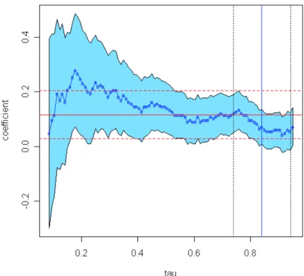
most. However, the exact nature of this bias is unknown in terms of quantiles. Figure 4 reports the entire quantile process and OLS for the above equation. Interestingly the effect of training on wages is monotonically decreasing inτ. The selection of the most likely quantile determines that as in the previous case ˆτ = 0.84.
[Figure 4]
In order to solve for the potential endogeneity, and following Abadie, Angrist, and Imbens (2002),z can be used as a valid instrument ford. The reason is that it is exogenous as it was a randomized experiment, and it is correlated withd(as mentioned earlier 60% of individuals undertook training when they were offered). The IV strategy is based on Chernozhukov and Hansen (2006, 2008) by considering the model
y−dα=xβ+zγ+u.
The IV method in QR proceeds as follows. Note that z does not belong to the model, as conditional on d, undertaking training, the offer has no effect on wages. Then, we construct a grid in α ∈ A, which is indexed by j for each τ ∈ (0,1) and we estimate the quantile
regression model for fixed τ
y−dαj(τ) =xβ+zγ+u.
This gives{βˆj(αj(τ), τ),ˆγj(αj(τ), τ)}, the set of conditional quantile regression estimates for
the new model. Next, we choose α by minimizing a given norm of γ (we use the Euclidean norm),
ˆˆ
α(τ) = argminα∈Akγ(α(τˆ ), τ)k.
Figure 5 shows the values of γ2 for the grids of α and τ. As a result we obtain the map
τ 7→{α(τ),ˆˆ β(ˆˆˆ α(τ), τ)≡β(τˆˆ ),ˆγ(ˆˆα(τ), τ)≡γ(τˆˆ )}.
[Figures 5]
condition corresponding the selection ofτ: ˆˆ τ =argminτ∈(0,1) 1−2τ τ(1−τ) − Pn i=1uˆˆi(τ) Pn i=1ρτ ˆˆ ui(τ)
where ˆˆui(τ) = yi −diα(τˆˆ )−x′iβ(τˆˆ )−ziγ(τˆˆ ). Figure 6 reports the IV estimates together
with the most likely quantile. Interestingly, the qualitative results are very much alike those of the value of the JTPA training offer. The IV least squares estimator for the effect of JTPA training gives a value of 0.116 (0.045) while IV median regression gives a much higher value of 0.142 (0.047). The most likely quantile continues to be 0.84 (0.053), which has an associated training effect of 0.072 (0.033). The ZQR effect continues to be smaller than the mean and median estimates. Therefore, the upper quantiles are more informative when analyzing the effects of JTPA training on log wages.
[Figure 6]
6
Conclusions
In this paper we show that the maximum likelihood problem for the asymmetric Laplace distribution can be found as the solution of a maximum entropy problem where we impose moment constraints given by the joint consideration of the mean and the median. We also propose an approximate Z-estimator method, which provides a parsimonious estimator that complements the quantile process. This provides an alternative interpretation of quantile regression and frames it within the maximum entropy paradigm. Potential estimates from this method has important applications. As an illustration, we apply the proposed estimator to a well-known dataset where quantile regression has been extensively used.
Appendix
A. Interpretation of the Z-estimator
In order to interpret θ0, we take the expectation of the estimating equations with respect to
the unknown true density. To simplify the exposition we consider a simple model without covariates: yi =α+ui. Our estimating equation vector is defined as:
E(Ψθ(y)) =E 1 σ (τ −1(y < α)) 1−2τ τ(1−τ) − (y−α) σ −1 σ + 1 σ2ρτ(y−α) = 0, and the estimator is such that
1 n n X i=1 Ψθ(yi) = 0
LetF(y) be the cdf of the random variable y. Now we need to find E[Ψθ(y)].
For the first component we have 1 σE[τ−I(y < α)] = 1 σ Z R (τ −1(y < α))dF(y) = 1 σ τ − Z α −∞ dF(y) = 1 σ(τ−F(α)). Thus if we set this equal to zero, we have
α=F−1(τ),
which is the usual quantile. Thus, the interpretation of the parameter αis analogous to QR if covariates are included.
For the third term in the vector, −σ1 + σ12ρτ(y−α), we have
E −1 σ + 1 σ2ρτ(y−α) = 0, that is, σ =E[ρτ(y−α)].
value of the loss function.
Finally, we can interpret τ using the second equation, E 1−2τ τ(1−τ) − (y−α) σ = 0, which implies that
1−2τ τ(1−τ) =
E[y]−F−1(τ)
σ .
Note thatg(τ)≡ τ1(1−−2ττ) is a measure of the skewness of the distribution (see also footnote 2). Thus, τ should be chosen to set g(τ) equal to a measure of asymmetry of the underline distribution F(·) given by the difference of τ-quantile with the mean (and standardized by σ). In the special case of a symmetric distribution, the mean coincides with the median and mode, such that E[y] = F−1(1/2) and τ = 1/2, which is the most probable quantile and a
solution to our Z-estimator.
B. Lemma A1
In this appendix we state an auxiliary result that states Donskerness and stochastic equicon-tinuity. Let F ≡ {ψθ(y, x), θ ∈ Θ}, and define the following empirical process notation for
w= (y, x): f 7→En[f(w)] = 1 n n X i=1 f(wi) f 7→Gn[f(w)] = 1 √ n n X i=1 (f(wi)−Ef(wi)).
We follow the literature using empirical process exploiting the monotonicity and bound-edness of the indicator function, the boundbound-edness of the moments of x and y, and that the problem is a parametric one.
Lemma A1. Under Assumptions A1-A4F is Donsker. Furthermore,
θ 7→Gnψθ(y, x)
is stochastically equicontinuous, that is sup kθ−θ0k≤δn Gnψθ(y, x)−Gnψθ 0(y, x) =op(1),
for any δn↓0.
Proof: Note that a classF of a vector-valued functionsf :x7→Rk is Donsker if each of
the classes of coordinates fi : x7→ Rk with f = (f1, ..., fk) ranging over F(i = 1,2, ..., k) is
Donsker (van der Vaart, 1998, p.270).
The first element of the vector is ψ1θ(y, x) = (τ −1(yi < x′iβ))xσi. Note that the
func-tional class A = {τ − 1{yi < x′iβ}, τ ∈ T, β ∈ B} is a VC subgraph class and hence
also Donsker class, with envelope 2. Its product with x also forms a Donsker class with a square integrable envelope 2·maxj|xj|, by Theorem 2.10.6 in van der Vaart and Wellner
(1996) (VW henceforth). Finally, the class F1 is defined as the product of the latter with
1/σ, which is bounded. Thus, by assumption A4 F1 is Donsker. Now define the process
h1 = (β, τ, σ) 7→ Gnψ1θ(y, x). Using the established Donskerness property, this process is
Donsker in l∞(F
1).
The second element of the vector is ψ2θ(y, x) = 1−2τ τ(1−τ)− (yi−x′iβ) σ . Define H = {(yi − x′ iβ), β ∈ B}. Note that |(yi−x′iβ1)−(yi−x′iβ2)|=|x′i(β2−β1)| ≤ kxikkβ2−β1k,
where the inequality follows from Cauchy-Schwartz inequality. Thus by Assumptions A3-A4 and Example 19.7 in van der Vaart (1998) the class H is Donsker. Moreover, H belongs to a VC class satisfying a uniform entropy condition, since this class is a subset of the vector space of functions spanned by (y, x1, ..., xp), wherep is the fixed dimension of x, so Lemma
2.6.15 of VW shows the desired result. Thus, by Example 2.10.23 (and Theorem 2.10.20) in VW the class defined by 1/σ H is Donsker, because the envelope of H (|y|+const∗ |x|) is square integrable by assumptions A3-A4. Thus F2 is Donsker. Using the same arguments
as in the previous case we can define h2 = (β, τ, σ) 7→ Gnψ2θ(y, x), and by the established
Donskerness property, this process is Donsker in l∞(F
2).
The third element of the vector is ψ3θ(y, x) = $ −1 σ + 1 σ2ρτ(yi−x′iβ) . Consider the following empirical process defined by J = {ρτ(yi −x′iβ), τ ∈ T, β ∈ B}. This is Donsker
by an application of Theorem 2.10.6 in VW. Finally, as in the previous cases define h3 =
(β, τ, σ)7→Gnψ3θ(y, x), and by the established Donskerness property, this process is Donsker
inl∞(F
3).
Now we turn our attention to the stochastic equicontinuity. The process θ 7→Gnψθ(y, x)
is stochastically equicontinuous over Θ with respect to a L2(P) pseudometric.6 First, as in
Angrist, Chernozhukov, and Fern´andez-Val (2006) and Chernozhukov and Hansen (2006), we define the distance d as the following L2(P) pseudometric
d(θ′, θ′′) =pE([ψθ′ −ψθ′′]2).
Thus, as kθ−θ0k →0 we need to show that
d(θ, θ0)→0, (28)
and therefore, by Donskerness of θ7→GnΨθ(y, x), we have Gnψθ(y, x) = Gnψθ 0(y, x) +op(1), that is sup |θ−θ0|≤δn kGnψθ(y, x)−Gnψθ 0(y, x)k=op(1).
To show (28), first note that
d(θ′, θ) = pE([ψ1θ′−ψ1θ]2) = s Eh(τ′−1(y−xβ′))x σ′ −(τ−1(y−xβ)) x σ i2 ≤h E 1 σ′(τ ′−1(y−xβ′))− 1 σ1(τ −(y−xβ)) 2(2+ǫ) ǫ !(2+ǫǫ) ·$ E(|x|2)2+2ǫ 2 (2+ǫ)i 1 2 = E ( τ′ σ′ − τ σ) + ( 1 σ1(y ≤xβ)− 1 σ′1(y≤xβ′)) 2(2+ǫ) ǫ !2(2+ǫǫ) ·$ E(|x|2)2+2ǫ 1 (2+ǫ) ≤h E τ′ σ′ − τ σ 2(2+ǫǫ) !2(2+ǫǫ) + E 1 σ1(y≤xβ)− 1 σ′1(y≤xβ′) 2(2+ǫǫ) !2(2+ǫǫ) i ·$ E(|x|2)2+2ǫ 1 (2+ ≤h τ′ σ′ − τ σ + E g¯·x ′(β′ σ′ − β σ) 2(2+ǫǫ) i ·$ Ekxk2+ǫ(2+1ǫ) ≤h τ′ σ′ − τ σ + ¯ gEkxk β′ σ′ − β σ 2(2+ǫǫ) i ·$ Ekxk2+ǫ(2+1ǫ) ,
third is a Taylor expansion as in Angrist, Chernozhukov, and Fern´andez-Val (2006) where ¯g is the upper bound of g(y|x) (using A2), and the last is Cauchy-Schwarz inequality.
Now rewrite ψ2θ(y, x) =
σ 1−2τ τ(1−τ) −(y−x′β) and d(θ′, θ) =pE([ψ2θ′ −ψ2θ]2) = s E h σ′ 1−2τ′ τ′(1−τ′)−(y−x′β′)−σ 1−2τ τ(1−τ)+ (y−x′β) i2 = s E σ′ 1−2τ′ τ′(1−τ′) −σ 1−2τ τ(1−τ) + (x′(β−β′)) 2 ≤ E σ ′ 1−2τ′ τ′(1−τ′)−σ 1−2τ τ(1−τ) 21/2 +$ E|x′(β−β′)|21/2 ≤ E σ ′ 1−2τ′ τ′(1−τ′)−σ 1−2τ τ(1−τ) 21/2 +kβ′−βk$ Ekxk21/2 ,
where the first inequality is given by Minkowski’s inequality (E|X+Y|p)1/p≤(E|X|p)1/p+
Finally, rewrite ψ3θ(y, x) = (−σ+ρτ(y−x′β)), and thus d(θ′, θ) = pE([ψ3θ′−ψ3θ]2) = s E h −σ′+ρτ′(y−xβ′) +σ−ρτ(y−xβ) i2 = s E h −σ′+σ+ρτ′(y−xβ′)− 1 σ2ρτ(y−xβ) i2 ≤ q E(−σ′ +σ)2+ s E h ρτ′(y−xβ′)−ρτ(y−xβ) i2 = q E(−σ′+σ)2 + s E h ρτ′(y−xβ′)−ρτ′(y−xβ) +ρτ′(y−xβ)−ρτ(y−xβ) i2 ≤ |σ−σ′|+ r E kx(β′−β)k+|τ′−τ|(y−xβ)2 ≤ |σ−σ′|+ r E kxkkβ′−βk+|τ′−τ|(y−xβ)2 ≤ |σ−σ′|+E kxkkβ′−βk21/2 +E |τ′−τ|(y−xβ)21/2 =|σ−σ′|+kβ′−βk$ Ekxk21/2 +|τ′−τ|$ E[(y−xβ)]21/2 ≤const·(|σ−σ′|+kβ′−βk+|τ′−τ|),
where the first inequality is is given by Minkowski’s inequality, the second inequality is given by QR check function properties as ρτ(x+y)−ρτ(y)≤2|x|and ρτ1(y−x′t)−ρτ2(y−x′t) =
(τ2 −τ1)(y−x′t). Third inequality is Cauchy-Schwarz inequality. Fourth is Minkowski’s
inequality. Last inequality uses assumption A4.
Thus, kθ′−θk →0 implies thatd(θ′, θ)→0 in every case, and therefore, by Donskerness of θ 7→Gnψθ(y, x) we have that
sup kθ−θ0k≤δn
kGnψθ(y, x)−Gnψθ
References
Abadie, A., J. Angrist, and G. Imbens (2002): “Instrumental Variables Estimates of the Effect of Subsidized Training on the Quantiles of Trainee Earnings,” Econometrica, 70, 91–117.
Angrist, J., V. Chernozhukov, and I. Fern´andez-Val(2006): “Quantile Regression under Misspecification, with an Application to the U.S. Wage Structure,” Econometrica, 74, 539–563.
Bloom, H. S. B., L. L. Orr, S. H. Bell, G. Cave, F. Doolittle, W. Lin, and
J. M. Bos (1997): “The Benefits and Costs of JTPA Title II-A programs. Key Findings from the National Job Training Partnership Act Study,”Journal of Human Resources, 32, 549–576.
Chernozhukov, V., I. Fern´andez-Val, and B. Melly (2009): “Inference on counter-factual distributions,” CEMMAP working paper CWP09/09.
Chernozhukov, V., andC. Hansen(2006): “Instrumental Quantile Regression Inference for Structural and Treatment Effects Models,” Journal of Econometrics, 132, 491–525.
(2008): “Instrumental Variable Quantile Regression: A Robust Inference Ap-proach,”Journal of Econometrics, 142, 379–398.
Ebrahimi, N., E. S. Soofi, and R. Soyer (2008): “Multivariate Maximum Entropy Identification, Transformation, and Dependence,” Journal of Multivariate Analysis, 99, 1217–1231.
Firpo, S. (2007): “Efficient Semiparametric Estimation of Quantile Treatment Effects,”
Econometrica, 75, 259–276.
Geraci, M., and M. Botai (2007): “Quantile regression for longitudinal data using the asymmetric Laplace distribution,” Biostatistics, 8, 140–154.
He, X.,andQ.-M. Shao(1996): “A General Bahadur Representation of M-Estimators and its Applications to Linear Regressions with Nonstochastic Designs,”Annals of Statistics, 24, 2608–2630.
(2000): “Quantile regression estimates for a class of linear and partially linear errors-in-variables models,”Statistica Sinica, 10, 129–140.
Hinkley, D. V., and N. S. Revankar (1977): “Estimation of the Pareto Law from Underreported Data: A Further Analysis,” Journal of Econometrics, 5, 1–11.
Huber, P. J.(1967): “The Behavior of Maximum Likelihood Estimates Under Nonstandard Conditions,” inFifth Symposium on Mathematical Statistics and Probability, pp. 179–195. Unibersity of California, Berkeley, California.
Kitamura, Y., and M. Stutzer (1997): “An Information-Theoretic Alternative to Gen-eralized Method of Moments Estimation,”Econometrica, 65, 861–874.
Koenker, R. (2005): Quantile Regression. Cambridge University Press, Cambridge.
Koenker, R., and G. W. Bassett (1978): “Regression Quantiles,” Econometrica, 46, 33–49.
Koenker, R., and J. A. F. Machado (1999): “Godness of Fit and Related Inference Processes for Quantile Regression,” Journal of the American Statistical Association, 94, 1296–1310.
Koenker, R.,andZ. Xiao(2002): “Inference on the Quantile Regression Process,” Econo-metrica, 70, 1583–1612.
Komunjer, I. (2005): “Quasi-maximum likelihood estimation for conditional quantiles,”
Journal of Econometrics, 128, 137–164.
(2007): “Asymmetric Power Distribution: Theory and Applications to Risk Mea-surement,” Journal of Applied Econometrics, 22, 891–921.
Kosorok, M. R. (2008): Introduction to Empirical Processes and Semiparametric Infer-ence. Springer-Verlag Press, New York, New York.
Kotz, S., T. J. Kozubowski, and K. Podg´orsk (2002a): “Maximum Entropy Char-acterization of Asymmetric Laplace Distribution,”International Mathematical Journal, 1, 31–35.
(2002b): “Maximum Likelihood Estimation of Asymmetric Laplace Distributions,”
Annals of the Institute Statistical Mathematics, 54, 816–826.
LaLonde, R. J. (1995): “The Promise of Public-Sponsored Training Programs,” Journal of Economic Perspectives, 9, 149–168.
Machado, J. A. F. (1993): “Robust Model Selection and M-Estimation,” Econometric Theory, 9, 478–493.
Manski, C. F. (1991): “Regression,” Journal of Economic Literature, 29, 34–50.
Park, S. Y., and A. K. Bera (2009): “Maximum entropy autoregressive conditional heteroskedasticity model,”Journal of Econometrics, 150, 219–230.
Schennach, S. M. (2008): “Quantile Regression with Mismeasured Covariates,” Econo-metric Theory, 24, 1010–1043.
Soofi, E. S., and J. J. Retzer (2002): “Information Indices: Unification and Applica-tions,”Journal of Econometrics, 107, 17–40.
van der Vaart, A.(1998): Asymptotic Statistics. Cambridge University Press, Cambridge.
van der Vaart, A., and J. A. Wellner (1996): Weak Convergence and Empirical
Processes. Springer-Verlag, New York, New York.
Wei, Y., and R. J. Carroll (2009): “Quantile regression with measurement error,”
Journal of the American Statistical Association, 104, 1129–1143.
Yu, K.,and R. A. Moyeed(2001): “Bayesian quantile regression,”Statistics & Probability Letters, 54, 437–447.
Yu, K., and J. Zhang (2005): “A three-parameter asymmetric Laplace distribution and its extension,”Communications in Statistics - Theory and Methods, 34, 1867–1879.
Table 1: Location-Shift Model: Bias and RMSE ZQR QR (Median) OLS N(0,1) Bias 0.0007 −0.0004 0.0008 RMSE 0.0904 0.0899 0.0710 ˆ τ 0.501 − − t3 Bias 0.0012 −0.0008 0.0014 RMSE 0.1133 0.0967 0.1217 ˆ τ 0.498 − − χ2 3 Bias −0.0021 0.0024 0.0020 RMSE 0.1419 0.1892 0.1801 ˆ τ 0.081 − − ALPD Bias 0.0001 0.0001 0.0001 (τ = 0.5) RMSE 0.0638 0.0549 0.0710 ˆ τ 0.499 − − ALPD Bias −0.0008 −0.0001 0.0003 (τ = 0.25) RMSE 0.0718 0.0860 0.0917 ˆ τ 0.248 − −
Table 2: Location-Scale-Shift Model: Bias and RMSE ZQR QR (Median) OLS N(0,1) Bias 0.0015 0.0036 0.0037 RMSE 0.2209 0.1461 0.1365 ˆ τ 0.499 − − t3 Bias −0.0005 0.0002 −0.0052 RMSE 0.2457 0.1460 0.2565 ˆ τ 0.501 − − χ23 Bias −0.0004 0.0076 0.0089 RMSE 0.5087 0.2833 0.3788 ˆ τ 0.086 − − ALPD Bias −0.0010 −0.0001 −0.0013 (τ = 0.5) RMSE 0.1455 0.0845 0.1459 ˆ τ 0.501 − − ALPD Bias 0.0051 0.0004 0.4076 (τ = 0.25) RMSE 0.1331 0.1429 0.4505 ˆ τ 0.248 − −
Table 3: JTPA offer
ZQR [ˆτ = 0.84] OLS Median regression Intercept 9.894 (0.059) 8.814 (0.088) 9.188 (0.086) JTPA offer 0.045 (0.022) 0.075 (0.032) 0.100 (0.033) FEMALE 0.301 (0.023) 0.259 (0.030) 0.260 (0.031) HSORGED 0.201 (0.025) 0.267 (0.034) 0.297 (0.037) BLACK -0.102 (0.026) -0.121 (0.036) -0.175 (0.039) HISPANIC -0.032 (0.034) -0.034 (0.050) -0.025 (0.051) MARRIED 0.129 (0.025) 0.242 (0.036) 0.265 (0.034) WKLESS13 -0.255 (0.023) -0.598 (0.032) -0.556 (0.036) AGE2225 0.229 (0.057) 0.175 (0.084) 0.125 (0.080) AGE2629 0.285 (0.058) 0.192 (0.085) 0.131 (0.081) AGE3035 0.298 (0.057) 0.191 (0.084) 0.176 (0.080) AGE3644 0.320 (0.058) 0.130 (0.085) 0.173 (0.081) AGE4554 0.267 (0.064) 0.110 (0.094) 0.080 (0.092) ˆ τ 0.840 (0.051) 0.500 ˆ σ 0.249 (0.060) 0.538 (0.006)
Notes: 9872 observations. The numbers in parenthesis are the corresponding standard errors. JTPA offer: dummy variable for individuals that recived a JTPA offer; FEMALE: Female dummy variable; HSORGED:
dummy variable for individuals with completed high school or GSE; BLACK: race dummy variable; HISPANIC: dummy variable for hispanic; MARRIED: dummy variable for married individuals; WKLESS13: dummy variable for individuals working less than 13 weeks in the past year; AGE2225,
Figure 1: Linear Combination of |y−µ| and (y−µ) !! !" # " ! #$# #$% &$# &$% "$# "$% ' ! ( "#$"# !& "# !" % !"&# !"&& ) !"&"& )
Figure 2: JTPA offer: Quantile regression process and OLS
Notes: Quantile regression process (shaded area), OLS (horizonal lines) and estimated most informative quantile (vertical lines) with 95% confidence intervals.
Figure 3: JTPA offer: τ-score function
Notes: The τ-score function is τ1(1−−2ττ) −
Pn
i=1(yi−x′iβˆ(τ))
Figure 4: JTPA: Quantile regression process and OLS
Notes: Quantile regression process (shaded area), OLS (horizonal lines) and estimated most informative quantile (vertical lines) with 95% confidence intervals.
Figure 6: JTPA: IV Quantile regression process and IV OLS
Notes: Quantile regression process (shaded area), OLS (horizonal lines) and estimated most informative quantile (vertical lines) with 95% confidence intervals.