Adaptive Pattern Recognition for Tornado Detection
1
Learning Objectives:
• Students will learn how to develop a simple three layer neural network consisting of: a two node input layer, a one node output layer, and a hidden layer that connects the two and is governed by the least mean squares (LMS) algorithm. From these principles, Matlab’s neural network toolbox will then be used to design meaningful, large-scale neural networks for realistic weather radar data senarios.
• Students will learn about the features need to detect a tornado using Level I data, which differs from conventional Level II techniques. The broad and flat spectra of the Level I data will be explored.
• Students will train a large-scale neural network to recognize the broad and flat Doppler spectrum associated with tornadoes. The students will examine a diverse class of artificial neural networks for the most efficient candidate. To do this, the students will look at their architecture, choice of kernel, training time, and the generalization ability of the classifier (how well it responds to new inputs).
2
Introduction
Enhanced tornado detection and tracking can prevent loss of life and property damage. The research WSR-88D (weather surveillance radar) locally operated by the National Severe Storms Laboratory (NSSL) in Norman has the unique capability of collecting massive volumes of time series data over many hours which provides a rich environment for evaluating new post-processing algorithms. With the advent of more memory and computing power, new state-of-the-art algo-rithms can be explored. In this laboratory, an approach of identifying tornado vortices in Doppler spectra is proposed and investigated through the use of neural networks. Once the coordinates of the tornado has been established, the research question becomes: how can students apply target tracking algorithms to a volume of radar data to make estimations about where the tornado is going?
2.1
Remote Sensing: the Weather Surveillance Radar
About one-third of the nation’s $10 trillion economy is sensitive to climate variability and weather [1–3]. Networked remote sensor systems, such as the ubiquitous WSR-88D (Weather Surveillance Radar - 1988 Doppler) in Figure 1, comprise the approximately 150 weather radars in the continental U.S. that are in a national network to provide the bulk of the nation’s weather information [4, 5]. The research WSR-88D (known as KOUN within the national network) oper-ated by the National Severe Storms Laboratory in Norman has the unique capability of collecting massive volumes of Level I time series data over many hours. A unique feature of the KOUN is that it has a dual polarization capability and hence the two receivers. It can change modes from dual to single polarization. It should also be mentioned that there are 47 more terminal Doppler
weather radars (TDWRs) that are similar to the WSR-88D at airports throughout the nation. A prominent feature of the TDWR is that it can probe inside storms and measure dangerous wind shifts, such as those linked to windshear and downburst, which pose a threat to aircraft during take-off and landing [6]. Long-term warnings have improved greatly over the last five years and are now being used for critical decision making [7]. Further improvements are being aimed at providing longer warning lead times before severe weather events, better quantification of forecast uncertainties in hurricanes and floods, and tools for integrating probabilistic forecasts with other data sets [7].
Figure 1: Hardware architecture of the operational system. The research WSR-88D (KOUN) operated by the National Severe Storms Laboratory in Norman has the unique capability of col-lecting massive volumes of Level I time series data over many hours. A unique feature of the KOUN is that it has a dual polarization capability and hence the two receivers. It can change modes from dual to single polarization (this drawing is used with permission from Allen Zahari, NSSL).
Weather surveillance radars, particularly the WSR-88D, have shown to be an important tool to observe severe and hazardous weather remotely, and to provide operational forecasters prompt information of rapidly evolving phenomena [8]. One of the most extreme weather phenomena is the tornado which can produce destructive wind speeds as high as 140 m/s [9]. Early and accurate detection of tornadic vortices can increase the lead time for tornado warning to prevent loss of life and property damage. A key component of current tornado detection algorithms on WSR-88D radars is a search for the presence of strong localized azimuthal shear of the radial winds. However, because the radar sample volume increases with distance from the radar, the shear signature deteriorates as the range of the tornado increases. In this work, an independent approach of identifying tornado vortices in Doppler spectra is proposed and investigated. The Doppler spectrum reveals weighted velocity distribution within the radar volume. The Level II data (reflectivity, mean Doppler velocity, and spectrum width) is obtained by the first three
facilitate their identification when the shear signature becomes difficult to identify.
Doppler spectra of tornadoes have a distinct character that set them apart from other spectra. Flat and bimodal tornado spectral signature (TSS) have been shown using simulated data [11]. Although the history of tornado measurements is long, there have been only a few successes in obtaining spectra data. This is largely because neither the technology to process spectra, nor the technology to record voluminous amounts of time series data were available. The present day radar technology and computer resources are now advanced enough to study TSS in a systematic manner. As a pulsed Doppler radar intermittently radiates electromagnetic energy, it also receives energy that is reflected back to it from various targets. These targets may be rain drops, hail stones, birds, aircraft, and other meteorological and non-meteorological reflections. When the energy is received at the radar, these analog signals are digitized, and the result is known as Level 1 data. Unlike typical WSR-88D’s, the research WSR-88D (KOUN) operated by the National Severe Storms Laboratory (NSSL) is a pulsed Doppler radar that has the unique capability of collecting significant quantities Level I time series data over many hours. Doppler spectra can be obtained by processing these Level I data after the event. Data from a tornado outbreak in central Oklahoma on May 10, 2003 are presented in the “hands-on activities” section of this lab.
2.2
Doppler Spectra and Spectral Analysis
The mean Doppler velocity ¯v(R0) is defined by the following equation.
¯
v(R0) =
Z ∞ −∞
vSn(R0, v) dv (1)
where Sn(R0, v) is the Doppler spectrum normalized by the total power, where R0 is the
cen-ter of the radar volume, and where v is the radial velocity component. Therefore, the mean Doppler velocity is the the first moment of the spectrum, which is estimated from one realization (or probe volume). Level I data are produced by received reflected energy. That is, energy is reflected back to the radar when it bounces back from an object. These objects or targets are typically referred to as scatterers, since energy is scattered back to the radar. Here, a target is a considered to be a water droplet within a tornado. The Level I data are represented in a format called in-phase(I) andquadrature(Q). A one-dimensional Fourier transform can be used to transform these time-domain I and Q samples into the frequency domain or Doppler velocity spectrum. Three spectral moments of weather phenomena from the I and Q data are: 1.) the weather signal power which is an indication of reflectivity, 2.) the mean Doppler velocity, and 3.) spectrum width. Hence, reflectivities and mean Doppler velocities were obtained every half degree in azimuth using the autocovariance method [10]. This method yeilds results that are similar to spectral analysis, but it is more computationally efficient since only the first three moments are being computed.
2.3
Example Tornado
Current tornado detection algorithms rely on the difference of mean Doppler velocity between adjacent radar volumes in azimuth. Tornado spectra observed by the NSSL research WSR-88D (KOUN) located at Norman, Oklahoma on May 10, 2003 are analyzed. An F2-F3 tornado was reported approximately during the interval of time 9:30 - 10:00 pm (central time) starting south of Edmond, Oklahoma (more details of the tornado can be found from NOAA National Climate Data Center NCDC, http://www.ncdc.noaa.gov/oa/ncdc.html). Level I time series data were collected during the entire period of tornado. A well-defined hook signature and strong azimuthal
Figure 2: PPI of the WSR-88D reflectivity at 9:43 pm, May 10, 2003. The small box outlines the location of the region of interest. The data for the spectral calculations in Figure 5 originate from this box. The small white dots indicate the tornado damage path from the ground survey.
shear were observed at 6 km west and 39 km north of the radar, indicating the existence of a tornado. As noted by Brown [12], a hook-shaped relectivity feature, that is typically on the right rear flank of a severe storm, indicates the presence of a mesocyclone that has the potential of having a tornado form within it. From simulation and real data, it is clear that tornado can produce a broad and flat spectrum which is similar to white-noise spectrum. However, significant signal power still remains in the tornado spectrum.
2.4
Neural Networks
A feedforward backpropagation (FFB) network is a generalization of network architecture of Figure 3. The authors in [13] have shown that a three-layer FFB neural network with sigmoid transfer functions in the hidden layer and linear transfer functions in the output layer, can approximate any continuous function to an arbitrary precision. To minimize the squared mapping error, CG algorithms traverse the error surface along a set of conjugate directions. A set of vectors
p1,p2, ...,pn construct a conjugate system if there is a non-singular symmetricN×N matrixA,
such that pT
i Apj = 0, fori6=j, i= 1,2, ..., n. The authors in [14, 15] have shown that the exact
minimum of any quadratic function can be found by moving along a set of conjugate directions
p1,p2, ...,pn. Such a conjugate system can be constructed by first defining p1 = −g1, then
at the old weights, i.e. Wk, k= 2, ..., nand βk is given by βk = gT kgk gT k−1gk−1 . (2)
CG methods adaptively update the weights in a sequence of steps by moving along the conjugate directions Wk+1 = Wk +αkpk. The variable αk is called the learning rate parameter and
determines how far movements occur along each search direction. For a quadratic function, αk
can be analytically calculated to minimize the performance function along the search path as defined by the conjugate directions [16]. Thus
αk =− gT kgk gT k−1Akgk−1 . (3)
The variable Ak=∇2F(W) is the Hessian matrix for a quadratic function. It is noticed that
in many practical applications the performance function is a higher order function of hundreds of weight parameters. However, a local quadratic approximation can be achieved by applying Taylor expansion formula [16]. Finally, the SCG algorithm employs an approximation of the Hessian matrix to reduce computational time and complexity. See [17] for more details.
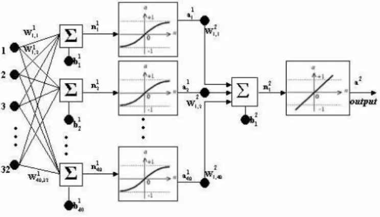
Figure 3: Sketch of the feedforward/backpropagation network which was employed. 32 input nodes were followed by 40 hidden neurons. The conjugate gradient algorithm was employed to train the 1280 weights of the first hidden layer, which are denoted byW1
. Similarly, the conjugate gradient algorithm was employed to train the 40 second-layer weights, which are denoted by W2
.
2.5
Data Preprocessing
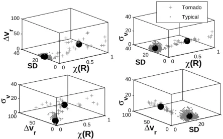
Figure 4 depicts how a clustering algorithm may be used to increase the class separability. Here, objects are clustered based on attributes into multiple partitions using the standard K-MEANS algorithm. The algorithm is a variant of the expectation-maximization algorithm in which the goal is to determine thek means of data generated from Gaussian distributions. It assumes that the object attributes form a vector space. The objective it tries to achieve is to minimize total intra-cluster variance. Based on these objects, a learning algorithm may be used to autonomously determine if a tornado is present or not.
0 0.5 1 0 20 400 50 100 χ(R) SD ∆ v r 0 0.5 1 0 20 400 20 40 χ(R) SD σ v Tornado Typical 0 0.5 1 0 50 1000 20 40 χ(R) ∆vr σ v 0 20 4 0 50 1000 20 40 SD ∆v r σ v
Figure 4: K-Means algorithms may be used to increase class separability, which improves the performance of the classifier or network.
3
Hands-On Activities
• Similar to our classroom discussions, derive a simple neural network that is based on a least mean squares (LMS) algorithm for its internal optimization. The network is to have three layers: input, hidden, and output. For this simple system, the input layer should have two nodes, while the output layer should have only one node. Show how such a system may be trained to mimic an OR gate, and present a graph illustrating the number of iterations that were needed for the training to become completed. After this, visit the Neural Network toolbox and familiarize yourself with it. It may be conveniently employed for large scale systems that have practical ramifications.
• Download this WSR-88D data:
– www.ou.edu/radar/data0305100331.m – www.ou.edu/radar/data0305100337.m – www.ou.edu/radar/data0305100343.m – www.ou.edu/radar/data0305100355.m – www.ou.edu/radar/data0305100034.m – www.ou.edu/radar/data0305100039.m
• Calculate the Doppler spectrum of each vector of 32 samples by taking the Fourier transform of the I and Q time-series samples, taking its magnitude squared, and expressing it in units of decibels. You may wish to implement further preprocessing of the data passing each Doppler spectrum through a low-pass digital filter (that you design). The smoothed Doppler spectra form the input feature vectors that are fed into your network.
• For the given range gates of data, the students will be responsible for carefully partitioning the data into two sets: one for training and one for classification (i.e. pattern recognition).
The student is also responsible for determining the number of input nodes and number of hidden nodes. Hint: the number of input nodes× the number of hidden nodes > 1000.
• Use ascaled conjugate gradient (SCG) training algorithm to adjust the weights in a neural network. SCG is a powerful extension of a class of optimization techniques known as the conjugate gradient (CG) methods. Your results should show how the training is used to adjust the weights of the neural network such that a desired mapping from input to the output is achieved. To solve this optimization problem, it is suggested that mapping error is to be defined as F(Wk) = e2(k) = [t(k)−a(k)]2, where Wk is the vector of network
weights and biases, e(k) is the error signal, t(k) is a vector of desired target outputs, and
a(k) is a vector current outputs of the network at the kth iteration. This activity may be
implemented using Matlab’s Neural Network toolbox. The students should explain his or her training and pattern recognition results using the network. For this exercise and data, a training curve for a working system is in Figure 5. As such, training times and false alarm rates should be discussed. Also make a drawing of architecture of the network showing all of the nodes and inter-connectivity relationships.
0 50 100 150 10−4 10−3 10−2 10−1 100 101 183 Epochs Training−Blue Goal−Black Performance is 0.000990751, Goal is 0.001
Figure 5: Error curve for a given number of training epochs.
• BONUS: In addition to a neural network, a support vector machine (SVM) classifier is to be designed and employed to identify the tornadoes and severe weather patterns using the I and Q data. In general, an SVM-based classifier evades the pitfalls of the traditional statistical learning algorithms, such as neural networks, by setting up a convex optimization problem with a single global minimum [18]- [22]. The student is required to show how using kernels and nonlinear mappings to higher dimensional spaces, the SVM classifier is
able to effectively handle nonlinear classification problems. Finally, the student should demonstrate how an SVM has the added advantage of reducing overfitting by constructing a maximum margin separating hyperplane in a higher dimensional feature space which ensures a small generalization error bound.
References
[1] Bureau of Economic Analysis, 2002: GDP by Industry. www. bea. gov /bea /dn2 /gpo. htm. [2] National Research Council, The Atmospheric Sciences Entering the Twenty First Century.
Washington, DC: National Academy Press, 1998.
[3] J. Dutton, “Opportunities and priorities in a new era for weather and climate services,”
Bulletin of American Meteorolgy Society, vol. 83, pp. 1303-1311, 2002.
[4] G. E. Klazura and D. A. Imy, “A description of the initial set of analysis products available from the NEXRAD WSR-88D system,” Bulletin of the American Meteorological Society, vol. 74, pp. 1293-1311, 1993.
[5] T. Crum and R. Alberty, “The WSR-88D and the WSR-88D operational support facility,”
Bulletin of the American Meteorological Society, vol. 74, pp. 1669-1687, 1993. [6] Terminal Doppler Weather Radar,
www.raytheon.com/newsroom/photogal/tdwr−h.htm
[7] National Research Council, Making Climate Forecasts Matter. Washington, DC: National Academy Press, 1999.
[8] R. Serafin and J. Wilson, “Operational weather radar in the United States: progress and opportunity,” Bulletin of the American Meteorological Society, vol. 81, pp. 501-518, 2000. [9] R. Davies-Jones, R. J. Trapp, and H. B. Bluestein, “Tornadoes and tornadic storms,” Severe
Convective Storms Conference, Amererican Meteorological Society. Boston, MA, pp. 167-221, 2001.
[10] R. J. Doviak and D. S. Zrni´c, Doppler Radar and Weather Observations. San Diego: Aca-demic Press, 1993.
[11] D. S. Zrni´c and R. J. Doviak, “Velocity spectra of vortices scanned with a pulsed-doppler radar,” Journal of Applied Meteorology, vol. 14, pp. 1531-1539. 1975.
[12] R. Brown, et. al., “Improved detection of severe storms using experimental fine-resolution WSR-88D measurements,” Weather and Forecasting, AMS, vol. 20, no. 1, pp. 3-14, February 2005.
[13] K. Hornik, M. Stinchcombe and H. White, “Multilayer feedforward networks are universal approximators,” Neural Networks, vol. 2, no. 5, pp. 359-366, 1989.
[14] L. Scales, Introduction to Non-Linear Optimization, New York: Springer-Verlag, 1985. [15] P. Gill, W. Murray and M. Wright, Practical Optimization, New York: Academic Press,
1981.
[16] M. Hagan, H. Demuth, M. Beale, Neural Network Design, ISBN 981-240-37-0. Colorado: University Publishing Service, 1996.
[17] M. Møller, “A scaled conjugate gradient algorithm for fast supervised learning,” Computer Science Department University of Aarhus Denmark, internal report, November 1990.
[18] B. Scholkopf and A. Smola, Learning with Kernels- Support Vector Machines, Regulariza-tion, Optimization and Beyond, MIT Press, 2002.
[19] J. Suykens, T. Van Gestel, J. De Brabanter, B. De Moor, and J. Vandewalle, Least Squares Support Vector Machines, World Scientific, Singapore, 2002.
[20] J. Suykens, L. Lukas, and J. Vandewalle, “Sparse least squares support vector machine classiers,” European Symposium on Articial Neural Networks (ESANN), pp. 37-42, 2000. [21] C. Fowlkes, S. Belongie, F. Chung, and J. Malik, “Spectral grouping using the Nystrom
method,IEEE Transactions on Pattern Analysis and Machine Intelligence vol. 26, no. 2, pp. 214-225, February 2004.
[22] P. Drineas and M. Mahoney, “On the Nystrom method for approximating a Gram matrix for improved kernel-based learning,”Journal of Machine Learning Research, vol. 6, pp. 2153-2175, 2005.