No. 2008–34
SEMIPARAMETRIC ROBUST ESTIMATION OF TRUNCATED
AND CENSORED REGRESSION MODELS
By Pavel
Č
ížek
March 2008
Semiparametric Robust Estimation of
Truncated and Censored Regression Models
Pavel ˇC´ıˇzek1
Department of Econometrics and Operation Research
Tilburg University, P.O. Box 90153, 5000 LE Tilburg, The Netherlands1
Abstract
Many estimation methods of truncated and censored regression models such as the maximum likelihood and symmetrically censored least squares (SCLS) are sensitive to outliers and data contamination as we document. Therefore, we propose a semipara-metric general trimmed estimator (GTE) of truncated and censored regression, which is highly robust and relatively imprecise. To improve its performance, we also propose data-adaptive and one-step trimmed estimators. We derive the robust and asymptotic properties of all proposed estimators and show that the one-step estimators (e.g., one-step SCLS) are as robust as GTE and are asymptotically equivalent to the original estimator (e.g., SCLS). The finite-sample properties of existing and proposed estimators are studied by means of Monte Carlo simulations.
Keywords: asymptotic normality, censored regression, one-step estimation, robust esti-mation, trimming, truncated regression
JEL codes: C13, C14, C21, C24
1
Introduction
In statistics and econometrics, more attention has been recently paid to techniques that can deal with data contamination and outliers, which can arise from miscoding or heterogeneity not captured or presumed in a model. Evidence for outliers and data contamination of a part of data and its adverse effects on estimators based on the least squares (LS) or maxi-mum likelihood (MLE) principles is provided, for example, by Gerfin (1996) in labor market
data, by Peracchi (1990) in household income-expenditure data, and by Sakata and White (1998) in financial time series. The need for estimation procedures insensitive to data con-tamination and large errors have been recognized by many authors, for example, Krasker and Welsch (1985), Hampel et al. (1986), Peracchi (1990), Krishnakumar and Ronchetti (1997), Ronchetti and Trojani (2001), Ortelli and Trojani (2005), and Bramati and Croux (2007). In this paper, we address robust estimation of truncated and censored regression models. On one hand, we document the sensitivity of existing (semi)parametric estimators to outliers and data contamination. On the other hand, we propose new highly robust semiparametric esti-mators of truncated and censored regression, derive their robust and asymptotic properties, and document in simulations that the proposed estimators provide robust and stable results without sacrificing the finite-sample performance.
The classical MLE estimation of truncated and censored regression is sensitive to de-partures from the assumptions of normality and homoscedasticity (Arabmazar and Schmidt, 1981). This gave rise to semiparametric estimators based on weaker identification assump-tions such as symmetrically trimmed least squares (STLS) and symmetrically censored least squares (SCLS), which rely on the conditional symmetry of errors (Powell, 1986), censored least absolute deviations (CLAD) estimator, which assumes the conditional median of errors being zero (Powell, 1984; Khan and Powell, 2001), and the mode regression (Lee, 1993). These concepts were later extended to the panel-data context (Honore, 1992; Honore and Powell, 1994). Further extensions include quantile regression (Portnoy, 2003), random censoring (Honore et al., 2002), and models with endogeneity (Hu, 2002; Honore and Hu, 2007). Alter-native methods based on nonparametric estimation of the density function include those by Gallant and Nychka (1989), Ichimura (1993), Lewbel (1998), and Lewbel and Linton (2002). Many truncated and censored regression estimators such as STLS or CLAD are often regarded to be robust not only in terms of identification assumptions, but also to outliers and data contamination because they employ “trimming” of regression residuals. This however holds only to a limited extent (Peracchi, 1990; Santos Silva, 2001) as we also document in this paper. This gave rise to a number of robust estimators of truncated and censored regression. For example, Peracchi (1990), Zhou (1992), Ren and Gu (1997), and Ren (2003) proposed various robust M-estimators for censored data, which bound the MLE score function to achieve lower sensitivity to extreme observations. Adjusting MLE however imposes strong
identification assumptions as MLE itself and the methods cannot be applied under random regressors and heteroscedasticity, for instance. Additionally, the robustness of M-estimators is typically very limited as the number of explanatory variables increases (Maronna et al., 1979) unless model-independent trimming of observations is used. Although the second concern could be eliminated by using a robust truncated MLE (ˇC´ıˇzek, 2007b; Marazzi and Yohai, 2004), the strong identification assumptions inherent to MLE are still present. Therefore, Debruyne et al. (2008) applied the concept of regression depth (Rousseeuw and Hubert, 1999) to censored quantile regression to create a robust alternative of CLAD. This method is however of a limited use given that there is no asymptotic theory, linear-regression depth was studied only in the i.i.d. case, and even a reliable computational algorithm does not exist.
In this paper, we propose robust estimators of truncated and censored regression, which are based on the STLS and SCLS estimators in order to construct semiparametric robust methods under weak identification assumptions (although the proposed concept can be ap-plied also to CLAD and other semiparametric estimators). In the truncated-regression case, we start from STLS, which symmetrically trims regression residuals, and generalize it to “trimmed STLS” by including an additional kind of trimming, which protects against outly-ing observations (a data-adaptive choice of the trimmoutly-ing amount is proposed as well). As a by-product, a robust estimator of the residual variance in the truncated and censored re-gression is developed. In the censored-rere-gression case, this approach is not applicable, and therefore, we propose the one-step SCLS, which performs one step of the SCLS computational algorithm starting from an initial robust estimator, for example, the trimmed STLS. Perform-ing just one step preserves robust properties of the initial estimator, whereas usPerform-ing the SCLS iterative formula allows to employ information from all sample observations. Next, we study both robust and asymptotic properties of all proposed estimators, and in particular, we show that the data-adaptive and one-step estimators are asymptotically equivalent to the original STLS and SCLS if there are no outlying observations. Although we mostly restrict ourselves to cross-sectional models, the proposed estimation methods can be straightforwardly gener-alized to CLAD, panel data, and other models considered in the above discussed literature on extensions of STLS, SCLS, and CLAD estimators.
The paper is organized in the following way. We first introduce some existing estimators of truncated and censored regression and basic concepts regarding the robust estimation in
Section 2. The proposed robust estimators are introduced in Section 3, where we also study their robust properties. The asymptotic distributions of all proposed methods are derived in Section 4. Finally, all estimation methods are compared in finite samples by means of Monte Carlo simulation in Section 5. The proofs are provided in the Appendix.
2
Estimation of truncated and censored regression
Let us now introduce various parametric and semiparametric estimators of truncated and censored regression and discuss their robust properties (Sections 2.1). Later, we introduce the concept of the general trimmed estimator (GTE), which will render the robust alternatives to some well-known estimators of truncated and censored regression (Sections 2.2).
2.1 Truncated and censored regression We consider the latent linear regression model
yi∗=x>i β0+εi, (1)
where y∗
i ∈ R is the latent (unobservable) response variable, xi ∈ Rp represents a vector of
explanatory variables (including intercept),β0 denotes the true value of the parameter vector
β ∈Rp, andεi is the latent error term with standard deviationσ =
p
var(εi). Without loss
of generality, we assume that the truncation or censoring occurs at zero from below. In the case of truncation, this means that the we observe only data points (yi, xi) = (y∗
i, xi) such
thaty∗
i >0; this truncated model will be denoted by TM. In the case of censoring, we observe
data points (yi, xi) with responseyi = max{yi∗,0}; the resulting modelyi = max{x>i β+εi,0}
will be referred to as CM.
Denoting di = I(yi > 0), the parameter vector β0 can be estimated by MLE, which
maximizes in the truncated-regression case (model TM)
lnLn(β, σ) = n X i=1 n lnfσ∗(yi−x>i β)−[1−lnFσ∗(0−x>i β)] o (2)
and in the censored-regression case (model CM) lnLn(β, σ) = n X i=1 n dilnfσ∗(yi−x>i β) + (1−di) lnFσ∗(0−x>i β) o , (3)
where we typically assume f∗
σ(t) = φ(t/σ) and Fσ∗(t) = Φ(t/σ) (φ and Φ represent the
standard normal density and distribution functions, respectively).
Since this MLE estimation is extremely sensitive to the violation of distributional assump-tions (Arabmazar and Schmidt, 1982), many alternative semiparametric estimators have been proposed. In the case of truncation, Powell (1986) proposed the STLS estimator minimizing
1 n n X i=1 [yi−max(yi/2, x>i β)]2, (4)
which relies on the conditional symmetry of theεi distribution. The same assumption in the
censored regression model leads to the SCLS estimator minimizing (Powell, 1986) 1 n n X i=1 n [yi−max(yi/2, x>i β)]2+I(yi >2x>i β)[(yi/2)2−max(0, x>i β)2] o . (5)
Other alternatives in the context of censored regression are, for example, the CLAD estimator (Powell, 1984), which is based on the conditional median restriction, and various semipara-metric estimators based on nonparasemipara-metric estimation of the density function (Gallant and Nychka, 1989; Lewbel and Linton, 2002). In this paper, we concentrate on the STLS and SCLS estimators, but many results are valid for or can be generalized to many other estima-tors of truncated and censored regression models such as CLAD or extensions of STLS and SCLS (e.g., Honore, 1992; Honore and Powell, 1994).
The discussed semiparametric estimators, STLS and SCLS, are often considered to be robust to data contamination because the symmetric trimming places an upper bound on the contribution of each observation to the objective function. In the case of STLS, for example, the contribution of an observation (yi, xi) cannot exceed (yi/2)2, see (4). We will however
document that all introduced estimators can be arbitrarily biased (towards zero or infinity) by data contamination anyway.
To formulate a result concerning the global robustness of truncated- and censored-regression estimators, we have to introduce a formal definition of the breakdown point, which measures
the smallest fraction of observations that, added at appropriate locations, can make the esti-mator“useless.” For the sake of simplicity, we consider independent and identically distributed observations (yi, xi)ni=1 (the breakdown point under dependence is generally model-specific;
see Genton and Lucas, 2003). The finite-sample breakdown point of a truncated or censored regression estimator ˆβn(Zn) at sample Zn = (xi, yi)ni=1 can be then defined as (Rousseeuw,
1997) ²∗n= 1 nmin ( m∈N0 : sup Zn0 kβˆn(Zn0)k=∞ ) , (6)
whereZn0 represents samples obtained fromZnby replacing anym observations by arbitrary values. The asymptotic breakdown point of the estimator ˆβnis then the corresponding limit ²∗= lim
n→∞²∗n (it usually exists and is independent of the data-generating process for
cross-sectional data). The breakdown point of a scale estimator ˆσn(Zn) can be defined similarly:
²∗n= 1 nmin ( m∈N0 : inf Zn0 kˆσn(Z 0 n)k= 0 or sup Zn0 kσˆn(Z 0 n)k=∞ ) .
Now, we show that the breakdown points of MLE, STLS, and SCLS in the truncated and censored regression models are asymptotically equal to zero, especially if data contamination includes leverage points, that is, observations with large values of explanatory variables (this result can be proved in the same way also for CLAD and other censored-regression estimators). Additionally, let us note that proving supZ0
nk
ˆ
βn(Zn0)k=∞in (6) does not necessarily imply that the slope estimates have to diverge: in the proof of the following theorem, we construct samplesZn0 such that all slope estimates become arbitrarily close to zero.
Theorem 1 Let (xi, yi)ni=1 be a sequence of independent and identically distributed random vectors from the truncated-regression model TM or censored-regression model CM. We assume that the data are almost surely in a general position for n >2p and that the models include intercept. Then the finite-sample breakdown points of the MLE and STLS estimators in truncated regression and of the MLE and SCLS estimators in censored regression are smaller than or equal to ²∗n= 2p/n, which tends to²∗= 0 asn→ ∞.
2.2 General trimmed estimator
The parametric and semiparametric estimators of the truncated and censored regression mod-els TM and CM are sensitive to outlying observations, especially those with high leverage (see
the proof of Theorem 1). One of traditional solutions reducing or eliminating this sensitiv-ity in (non)linear regression amounts to downweighting or trimming observations that have large regression residual (e.g., Rousseeuw, 1985). We will introduce here a generalization of this concept – the general trimmed estimation – to facilitate the proposal of semiparametric robust regression estimators later in Section 3.
To address high sensitivity of the MLE- and LS-based methods to outlying or misspecified observations, ˇC´ıˇzek (2007b) proposed the concept of general trimmed estimation (GTE). Given a sample (xi, yi)n
i=1 and an estimation methodT that minimizes the objective function
of the formPni=1s(xi, yi;β) overβ ∈B, wheres(xi, yi;β) represents a loss function identifying the true valueβ0 of parameter vectorβ, one typically knows that small values ofs(x
i, yi;β)
represent likely observations under a given model (“good fit,” e.g., small squared residuals) and large values of s(xi, yi;β) correspond to unlikely values (“bad fit,” e.g., large squared
residuals). For example, if we observe y∗
i and xi in the latent linear model (1), we could
estimate it by LS usings(xi, yi∗;β) = (y∗i −x>i β)2; the small residuals would then mean that
a given observation is fit by the model well and vice versa.
To create a method insensitive to outliers and observations badly explained by the model, GTE minimizes an objective function from which the unlikely observations (i.e., observations with large values ofs(xi, yi;β)), are trimmed away. In this simple case, the general trimmed
estimator ˆβn(GT E-T,h) obtained from the estimation methodT can therefore be defined as
ˆ βn(GT E-T,h) = arg min β∈B hn X j=1 s[j](β), (7)
where s[j](β) represents the jth smallest order statistics of s(xi, yi;β), i = 1, . . ., n. Thus,
the GTE estimate minimizes the loss ofhn most likely observations under a given parametric
model, where the trimming constant satisfiesn/2< hn≤n. Note that the trimming constant
hndetermines the insensitivity to outliers and breakdown point of GTE because (7) indicates that n−hn observations with the largest losses do not directly affect the estimator. In the (non)linear regression, GTE combined with LS (GTE-LS) results in the well-known least trimmed squares estimator (LTS; Rousseeuw, 1985), which achieves the maximum asymptotic breakdown point 1/2 if hn = [(n+ 1)/2] +p (Rousseeuw and Leroy, 2003; Stromberg and
3
Robust estimation of truncated and censored regression
In Section 2, we have seen that many well-known estimators of truncated and censored re-gression are sensitive to outliers and data contamination and have asymptotically breakdown points equal to zero (Theorem 1). At the same time, a general GTE concept of creating robust estimators was introduced. Since MLE relies on strong identification assumptions, we start by applying GTE to the less-restrictive STLS estimator in truncated regression (Section 3.1). Because trimming of observations usually results in a substantial increase of the variance of estimates, we also propose a data-adaptive procedure for the choice of trimming amount to eliminate or minimize the relative-efficiency loss (Section 3.2). Finally, we discuss how the proposed robust estimation methods can be extended to the SCLS estimator in the censored regression model (Section 3.3). The identification assumptions and asymptotic properties of all proposed methods will be studied later in Section 4.
3.1 Robust estimation of truncated regression models
To propose a robust alternative to the MLE and STLS estimators of the truncated-regression model TM, we start from STLS, which relies on relatively weak identification assumptions, and apply the GTE concept to STLS. More precisely, we propose the GTE-STLS estimator of the model TM defined by
ˆ β(GT E-ST LS,hn) n = arg min β∈B hn X j=1 s[j](β) = arg min β∈B hn X j=1 n [yi−max(yi/2, x>i β)]2 o [j] (8)
wheres[j](β) represents thejth smallest order statistics ofs(xi, yi;β) = [yi−max(yi/2, x>i β)]2,
i= 1, . . ., n. (Note that we could obviously define the same way a GTE counterpart of MLE.) An important feature of GTE-STLS is that it trims the observations with large absolute values of symmetrically trimmed residuals min{yi/2, yi −x>i β} rather than only the observations
with observable residuals, 0≤x>
i β. Similarly to LTS, the proposed GTE-STLS trims exactly
n−hnobservations from the objective function, where [(n+ 1)/2] +p≤hn≤n, and can thus
survive contamination of up to [(n−hn)/n] percent of data (cf. Stromberg and Rupert, 1992),
3.2 Adaptive choice of trimming
The GTE-STLS estimator proposed in Section 3.1 is a robust alternative to MLE and STLS. It is however well known that trimming 25% or 50% observations of the sample causes a substantial increase in the variance of estimates even in the linear regression (cf. ˇC´ıˇzek, 2007a) and we can thus expect en even more negative effect of trimming on the relative efficiency of the estimator in the truncated regression case. Therefore, we complement GTE-STLS by a data-adaptive choice of the trimming constant hn so that the smallest possible
amountn−hn of observations is trimmed from the objective function.
The adaptive choice of trimming is motivated by Gervini and Yohai (2002) and ˇC´ıˇzek (2007a), who studied the data-dependent trimming in the context of the linear regression model. It is therefore beneficial to describe the linear-regression case first. Provided that we obtain initial robust estimates ˆβn0 and ˆσ0n of the regression parameters β and standard deviationσ of regression residuals (e.g., by LTS withhn= [(n+ 1)/2] +pand by the median absolute deviation), the choice of trimming is done by comparing the empirical distribu-tion funcdistribu-tionG0
nof standardized absolute residuals|ri( ˆβn0)/σˆn0|and the distribution function
F|·|(z) = Φ(z)−Φ(−z), which describes behavior of |εi|under the assumption of normally
distributed errors, εi ∼N(0,1) (G0n is compared toF|·| because LS perform optimally under normality and outliers are extremely improbable under N(0,1)). Specifically, Gervini and Yohai (2002) proposed to measure the largest difference between G0
n and F|·| in the tail of the distributions,
dn= sup
t≥c
max{0, F|·|(t)−Gn0(tσˆn0)}, (9) where the cut-off point c equals 2.5 and ˆσ0
n = 1.4826·MADi=1,...,nri( ˆβn0) is the median
absolute deviation (MAD) estimate of the residual variance. Using this measure, ˇC´ıˇzek (2007a) proposed to estimate using LTS with the following data-dependent choice of trimming: han=n−[dnn]. The method performs very well under normality, heavy-tailed distributions,
and also under heteroscedasticity despite “assuming” the same distribution for all data in (9), see ˇC´ıˇzek (2007a).
To employ this idea in the truncated-regression case, we have to take into account that we do not fully observe the regression residuals y∗
i −x>i β. We can however compute
|ris(β0)| = |yi−x>i β0|/σ = |εi|/σ conditional on ξi = x>i β0/σ if the error term εi in the
latent model (1) is normally distributed,N(0, σ):
Fr|ξ(t|ξi =x>i β0/σ=ξ) = [Φ(t)−Φ(−t)]/[1−Φ(−ξ)] if 0≤t≤ξ, [Φ(t)−Φ(−ξ)]/[1−Φ(−ξ)] if|ξ|< t, 0 ift <−ξ;
(the result follows from the fact that observed error εi is truncated at−ξi =−x>i β0).
Next, we have to average the conditional distribution Fr|ξ across ξ, that is, across ob-servations with different values xi, to obtain an unconditional distribution. To obtain
con-servative estimates, we will use only observations likely under the assumption ε ∼N(0, σ). In particular, an observation with ξi = x>i β0/σ < 0 in a truncated sample of size n is
ob-served with probability 1−Φn(|ξ
i|) because εi/σ > |ξi| (Φn is the distribution function of
maxi=1,...,n[εi/σ]). Considering only observations that can appear in the sample with
prob-ability higher than some small α > 0, we have to impose condition 1−Φn(|ξ
i|) > α, that
is, ξi > −Φ−1(√n1−α) = C
n(α). The number of observations satisfying this condition will
be denoted nα =
Pn
i=1I{ξi > Cn(α)}. Note that Cn(α) → −∞ asymptotically and the
condition ξi> Cn(α) is thus always satisfied forn→ ∞.
Finally, denoting the distribution function of ξi =x>i β0/σ by Fξ (absolutely continuous
by assumption, see Section 4), the cumulative distribution functionFr,αof|ri(β0)|conditional
upon ξi =x>i β0/σ > Cn(α) can be expressed as Fr,α(t) =
R+∞
Cn(α)Fr|ξ(t|ξ)dFξ(ξ). Hence for
any t≥0, it holds that
Fr,α(t) = Z t max{−t,Cn(α)} Φ(t)−Φ(−ξ) 1−Φ(−ξ) dFξ(ξ) + Z ∞ t Φ(t)−Φ(−t) 1−Φ(−ξ) dFξ(ξ). Given initial estimates ˆβ0
n and ˆσ0n ofβ0 and σ and a sample (xi, yi)ni=1, an integral
Z A g(t, ξ)dFξ(ξ) = Z R g(t, ξ)I(ξ ∈A)dFξ(ξ) =E{g(t, ξi)I(ξi∈A)}
Fr,α(t) by Frn,α(t) = nˆ1 α n X i=1 Φ(t)−Φ(−x>i βˆn0/σˆ0n) 1−Φ(−x> i βˆn0/σˆ0n) I(max{−t, Cn(α)}< x>i βˆn0/σˆn0 < t) (10) + Φ(t)−Φ(−t) ˆ nα n X i=1 1 1−Φ(−x> i βˆn0/σˆn0) I(t≤x>i βˆn0/σˆ0n), where ˆnα = Pn
i=1I{x>i βˆn0/σˆn0 > Cn(α)}. Analogously to (9), we can then determine the
proportion of observations to be trimmed byha
n=n−[dnn] and
dn= sup
t≥cmax{0, Frn,α(t)−G
0
n(tσˆ0n)}, (11)
wherec= 2.5 andα= 0.001, for instance.
The only remaining issue is a robust estimate of ˆσ0
n, which was estimated using MAD
in the linear-regression case when responses are fully observed. Since the STLS estimator relies on the symmetry of the latent-error distribution and the usual identification assumption E(εi|xi) = med(εi|xi) = 0, the variance in the truncated case can be consistently estimated
using only observations “above” the regression line:
MAD(εi|xi) = med(|εi−med(εi|xi)||xi) = med(|εi||xi) = med(εi|xi, εi >0),
where the last equality follows from the symmetry of the distribution ofεi. Using observations with fully observable positive residuals, that is those with yi ≥ x>
i β0 ≥ 0, results in the
following estimate of the residual variance:
ˆ
σn0 = 1.4826·med{ri( ˆβn0) :yi≥x>i βˆn0 ≥0}. (12)
The practical application of the proposed adaptive choice of trimming consists of three steps: (i) an initial estimate ˆβ0
nand the corresponding residualsri( ˆβn0) are obtained by
GTE-STLS using trimming constanth0
n, for exampleh0n= [(n+ 1)/2] +p; (ii) the residual variance
is estimated by (12) and the trimming proportionha
n=n−[dnn] is determined using (11); (iii)
the final estimate ˆβn(AGT E−ST LS) = ˆβ(GT E−ST LS,h
a
n)
n is computed using GTE-STLS with the
data-dependent trimming constanthan. We refer to this estimate as the adaptive GTE-STLS (AGTE-STLS). The whole procedure is constructed so that AGTE-STLS is asymptotically
equivalent to STLS if errors are homoscedastic and normally distributed because the ref-erence distribution Fr(t) =
R
Fr|ξ(t|ξ)dFξ(ξ) in (11) is constructed under the assumption εi ∼ N(0, σ): hence, both Frn,α(t) → Fr(t) and Gn0(tσˆn0) → Fr(t), t ≥ 0, as n → ∞ if the
initial estimates are consistent ( ˆβ0
n → β0, ˆσ0n →σ, and Cn(α) = −Φ−1(n
√
1−α) → −∞for any fixedα∈(0,1) asn→ ∞). This means that AGTE-STLS with adaptive trimming uses all observations “compatible” with normality. Even though outliers are very unlikely under normality, we should make sure that such a data-dependent choice of trimming does not use more observations and improve the variance of estimates at cost of a lower robustness of the whole procedure. The following theorem therefore shows that the breakdown point of AGTE-STLS is not smaller than the breakdown of the initial robust estimator.
Theorem 2 Let (yi, xi)ni=1 be a sequence of independent and identically distributed random vectors, which are almost surely in a general position for n > 2p. Further, let ²0∗
n denote
the finite-sample breakdown point of an initial estimator ( ˆβ0
n,ˆσn0) of regression parameters and residual variance. Then the finite-sample breakdown point of the AGTE-STLS estimator is larger than or equal to ²0n∗ if the GTE-STLS estimators with trimming constants hn are identified for all [(n+ 1)/2] +p≤hn≤n.
(We will see in Section 4 that the identification assumptions of GTE-STLS are identical to those for STLS discussed in Powell (1986).)
3.3 Robust estimation of censored regression
In Sections 3.1 and 3.2, we introduced a robust (A)GTE-STLS estimator of truncated regres-sion. Using the same strategy, combining directly GTE and SCLS, does not however seem to be feasible in the censored regression model. Intuitively, the GTE type of trimming would invalidate the conditional mean or median restrictions. For example, if ε∗ conditional on x is symmetrically distributed around 0 on the whole real line andε= max{ε∗,−x>β}, SCLS relies on E[min{ε, x>β}I(0 < x>β)|x] = 0 (Powell, 1986), which does not hold once large values of|ε|are trimmed: E[min{ε, x>β}I(|ε| ≤K)I(0< x>β)|x]6= 0 for anyK > x>β. On the other hand, the proposed (A)GTE-STLS estimator can be directly applied in censored regression if only non-censored observations are used. Specifically, having a censored sample (xi, yi)ni=1, we can estimate the parameters of the model CM by applying AGTE-STLS to the
subsample (xi, yi)yi>0 of the original data. Such estimates will have a positive breakdown
point proportional to [(n−cn)/(2n)], where cn =
Pn
i=1I(yi = 0) denotes the number of
censored observations, because GTE-STLS can trim at most half of the n−cn observations
contained in the truncated sample (xi, yi)yi>0.
Despite the adaptive choice of trimming, the application of AGTE-STLS in censored re-gression is suboptimal since it neglects the information present in the censored observations with yi = 0. Since the (A)GTE-STLS provides already a robust estimator of censored
re-gression, we can however employ the so-called one-step estimation, which is often used for robust M-estimators of linear regression (Simpson et al., 1992; Welsh and Ronchetti, 2002). Since nonlinear methods such as M-estimators are computed using iterative optimization techniques, the one-step estimation employs an initial robust estimate ˆβ0
n as a starting point
to perform a single step of the iterative optimization procedure. The resulting estimator can then inherit robust properties of the initial estimator and asymptotic properties of the M-estimator (Simpson et al., 1992).
In the case of SCLS, the iterative computation algorithms were proposed by Powell (1986) and Santos Silva (2001). We discuss here only the first one, since the latter Newton-type algo-rithm is less stable and cannot preserve the robust properties of AGTE-STLS at an arbitrary sample. Powell’s algorithm relies on the moment conditionE[ximin{εi, x>i β0}I(x>i β0>0)] =
0, which holds under the conditional symmetry ofεigiven xi. Substitutingεi =yi−x>i β, we
can solve this moment condition for β and replacingβ0 by an initial estimate ˆβ0
n then leads
to the following estimate ˆβC
n (cf. Powell, 1986, equation (2.13)) ˆ βnC( ˆβ0n) = " 1 n n X i=1 xix>i I(x>i βˆn0 >0) #−1 1 n n X i=1 ximin{yi,2x>i βˆn0}I(x>i βˆn0 >0). (13)
Note that the inverted matrix has to be non-singular if SCLS is identified (see Section 4 and Powell, 1986, Assumption R). If the inverted matrix is singular, we just define ˆβC
n( ˆβn0) = ˆβn0.
Using the iterative formula (13) and (A)GTE-STLS as the initial estimator ˆβ0
n, we can now
propose robust one-step SCLS estimators of the censored regression model CM: ˆ
β(ON E−SCLS,hn)
n = βˆnC( ˆβn(GT E−ST LS,hn)), (14)
ˆ
the resulting estimators are referred to as ONE-SCLS.
Even though the one-step estimation seems to be necessary only in the context of censored regression, we can also use it in the context of truncated regression as an alternative to AGTE-STLS. The STLS estimator relies on the moment condition E[εixiI(εi < x>i β0)] = 0, which
holds under the conditional symmetry of εi given xi. Substituting εi = yi−x>i β, solving
this moment condition for β, and replacing β0 by an initial estimate ˆβn0 then produces the following iterative equation
ˆ βnT( ˆβn0) = " 1 n n X i=1 xix>i I(yi<2x>i βˆn0) #−1 1 n n X i=1 xiyiI(yi <2x>i βˆn0). (16)
We again have to assume that the STLS estimator is identified and that the inverted matrix is thus non-singular (see Section 4 and Powell, 1986, Assumption R and E2); otherwise,
ˆ
βnT( ˆβ0n) = ˆβn0. Using formula (16) and (A)GTE-STLS as the initial estimator ˆβn0, we can propose robust one-step STLS estimators of the truncated regression model TM defined by
ˆ
β(ON E−ST LS,hn)
n = βˆnT( ˆβn(GT E−ST LS,hn)), (17)
ˆ
βn(ON E−ST LS,A) = βˆnT( ˆβ(nAGT E−ST LS)); (18)
the method is referred to as ONE-STLS.
For both truncated and censored regression, we thus propose to use the robust GTE-STLS or AGTE-STLS estimators as the initial estimators and to perform one step of the iterative STLS or SCLS algorithm, (16) or (13). On one hand, the resulting STLS and ONE-SCLS estimators will always use all observations and thus more information from data. On the other hand, the one-step estimation preserves the breakdown point of the initial estimator as we show in the following theorem.
Theorem 3 Let (yi, xi)n
i=1 be a sequence of independent and identically distributed random vectors, which are almost surely in a general position forn >2p. Further, let²0∗
n denote the finite-sample breakdown point of an initial estimator βˆ0
n of regression parameters. Then the finite-sample breakdown points of the ONE-STLS and ONE-SCLS estimators are larger than or equal to ²0∗
n.
that AGTE-STLS will be less sensitive, in terms of bias, to outliers and data contamination because it can reject some observations from its objective function. On the other hand, ONE-STLS and ONE-SCLS could possibly exhibit smaller variances of estimates because they always use all available observations. A detailed comparison of all estimators by means of asymptotic properties and by means of Monte Carlo simulations follows in Sections 4 and 5.
4
Asymptotic properties
Let us now analyze the asymptotic properties of the proposed (A)GTE-STLS, ONE-STLS, and ONE-SCLS estimators. After introducing notation and assumptions needed for the asymptotic analysis, we will first find the asymptotic distribution of GTE-SCLS with the trimming constant being a fixed fraction of the sample,hn= [λn], whereλ∈(1/2,1i. Later,
we look at the asymptotic behavior of AGTE-SCLS, that is, GTE-SCLS with the adaptively chosen trimming, and finally, we study the asymptotic distributions of the proposed one-step estimators.
First, the (unconditional) distribution function of εi in model (1) is referred to asF and
its density function is denotedf, provided that it exists. A density function f of a random variable with zero mean will be called (strictly) unimodal if f(z1) ≥f(z2) (f(z1) > f(z2))
for any |z1| ≥ |z2|. Further, let us introduce the concept of β-mixing, which is central to
the distributional assumptions made here. A sequence of random variables{xi}i∈Nis said to
be absolutely regular (or β-mixing) if βm = supi∈NE{supB∈σf
i+m|P(B|σ
p
i)−P(B)| →0} as
m→ ∞, whereσ-algebrasσpi =σ(xi, xi−1, . . .) andσfi =σ(xi, xi+1, . . .); see Davidson (1994) for details. Numbers βm,m∈N, are called mixing coefficients.
Now, let us present the assumptions used to derive the asymptotic distribution of all proposed estimators.
Assumption A
A1 Random vectors (xi, yi)i∈N form a weakly stationary absolutely regular sequence with mixing coefficients βm satisfying mr/(r−2)(logm)2(r−1)/(r−2)βm → 0 as m → ∞ for
somer >2 and have finite rth moments. Moreover, letE{xix>i I(x>i β0 ≥γ0)}=Qbe
A2 Let{εi}i∈Nbe a sequence of independently distributed random variables, and conditional
onxi, let{εi}i∈Nbe symmetrically distributed with finite second moments,E(εi|xi) = 0
and var(εi|xi)<∞. The conditional distribution functionFi of εi given xi is assumed
to be absolutely continuous with its probability density function fi being bounded,
positive at 0, and continuously differentiable uniformly ini∈N. Additionally, the error densities fi have to be unimodal and strictly unimodal in some neighborhood of zero
uniformly ini∈N.
A3 The true parameterβ0 lies in the interior of a compact parametric spaceB.
The majority of Assumptions A correspond to Assumptions P, R, E1, and E2 used by Powell (1986) to analyze the asymptotic properties of STLS and SCLS. Compared to Powell (1986), we allow for dependence in data (Assumption A1), but additionally require the differentia-bility of the error density functions. Let us also note that, while the moment assumptions might look relatively strong on the first look, they can be weakened in some cases: (i) if only consistency of (A)GTE-STLS or ONE-SCLS is required, finite (2 +δ)th moments are sufficient and (ii) if (A)GTE-STLS is considered and there is a positive amount of trimming, hn = [λn] < n and λ < 1, only trimmed moments of all variables have to exist (cf. ˇC´ıˇzek,
2007b). Finally, note that the assumption of random carriers for all variables is made for the sake of simplicity and the results apply in the presence of deterministic variables as well.
Let us first derive the asymptotic distribution of (A)GTE-STLS.
Theorem 4 Let Assumption A hold. Then the GTE-STLS estimator βˆ(GT E−ST LS,hn)
n of the
model TM using trimming hn = [λn], λ∈(1/2,1i, is consistent and asymptotically normal, that is, √ n ³ ˆ β(GT E−ST LS,hn) n −β0 ´ F →N(0, V(λ))
as n→+∞. Furthermore, the asymptotic distribution of GTE-STLS does not change ifhan
is random (data-dependent) and ha
n/n→λ in probability asn→+∞.
An important consequence of Theorem 4 is that the asymptotic distribution does not depend on (random) trimmingha
n as long ashan/n→λin probability. Therefore, the
asymp-totic distribution of AGTE-STLS proposed in Section 3.2 is the same as for GTE-STLS with trimming [nlimn→∞(han/n)]. In particular, if the latent error term in (1) is homoscedastic
and normally distributed, ha
n/n= (n−[dnn])/n →1 as n→ ∞ as explained in Section 3.2
and the asymptotic distribution of AGTE-STLS is identical to that of STLS.
Next, although we proved the asymptotic normality of (A)GTE-STLS, we do not specify the precise form of the asymptotic variance matrixV(λ). Even though it could be formally derived, it does not have a computationally feasible form, especially under heteroscedasticity (cf. Powell, 1986, and the nontrivial asymptotic distribution of STLS itself). Hence, it has to be computed by a parametric or a robust nonparametric bootstrap, for instance (e.g., Hall and Presnell, 1999; Salibian-Barrera and Zamar, 2002).
Alternatively, one can use the GTE-STLS estimate only as a starting point and compute the one-step ONE-STLS or ONE-SCLS estimators. Although this could possibly increase bias due to outliers and data contamination, ONE-STLS and ONE-SCLS employ all information in a sample, and more importantly, are asymptotically first-order equivalent to STLS and SCLS as we show in the following theorem.
Theorem 5 Let Assumption A hold and let βˆn0 be a√n-consistent estimate of parametersβ
in the models TM and CM. Then the ONE-STLS estimator βˆn(ON E−ST LS) = ˆβnT( ˆβn0) of the model TM based on βˆ0
n and the ONE-SCLS estimator βˆn(ON E−SCLS) = ˆβnC( ˆβ0n) of the model CM based on βˆ0
n are first-order asymptotically equivalent to the STLS estimate βˆn(ST LS) and to the SCLS estimate βˆn(SCLS), respectively:
√
n( ˆβn(ON E−ST LS)−βˆn(ST LS))→0 and √n( ˆβn(ON E−SCLS)−βˆn(SCLS))→0
in probability as n→ ∞.
Theorem 5 documents the well-known fact that the asymptotic distribution of one-step estimators can be independent of the initial estimator. It also means that the proposed one-step estimators, ONE-STLS and ONE-SCLS, have the same asymptotic distributions as STLS and SCLS and the asymptotic variances by Powell (1986) can thus be applied as long as the number of observations is sufficiently large. See Section 5 for more details.
5
Finite-sample properties
In this section, we present a Monte Carlo study done to assess finite-sample behavior of the proposed GTE-STLS withhn= [(n+ 1)/2] +p, AGTE-STLS, ONE-STLS, and ONE-SCLS
estimators; note that ONE-STLS-0 and ONE-SCLS-0 will denote the one-step estimators based on GTE-STLS, whereas ONE-STLS-A and ONE-SCLS-A will refer to estimates using AGTE-STLS as the initial estimator. The proposed estimators are compared with MLE, STLS, and SCLS in the context of truncated regression (Section 5.1) and censored regression (Section 5.2).
In all cases, we generate data using a latent model (1), y∗
i =x>i β+εi,and subsequently,
we omit the observations with y∗
i <0 in the case of the truncated model TM or we setyi =
max{y∗
i,0}in the case of the censored model CM. The presented simulations, based on 1000
simulated samples, are done for sample sizesn= 100, 200, and 400 usingβ= (1,−1,1)> and εifrom various distributions (results however do not qualitatively change with the dimension
of β). In this setup, for example, n = 100 and x1i, x2i, εi ∼ N(0,1) lead to samples than
contain 17–40 observations withy∗
i ≤0 with probability more than 99%. We use the following
data generating processes, where x1i ∼N(0,1) and x2i ∼N(0,1) unless stated otherwise:
NORM: Clean Gaussian data,εi∼N(0,1).
DEXP: Data with errors following a double-exponential distribution,εi ∼DExp(1).
STD(d): Data with errors from a heavy-tailed distribution, εi ∼t(d), where t(d) denotes
the Student distribution withddegrees of freedom.
HETX: Data with heteroscedastic errors, εi ∼ N(0, e2x1), where variance depends on
covariate values.
HETZ: Data with heteroscedastic errors,εi ∼N(0, z), where variance depends on
unob-servablez∼U(0.25,4) and U(a, b) denotes the uniform distribution on (a, b). OUT(a;l1, l2): Data contaminated by [an], a ≥0, outliers at location (l1, l2) ∈ R2.
Specifi-cally, a fraction 1−a of observations satisfies x1i ∼ N(0,1), x2i ∼ N(0,1), and
εi ∼ N(0,1), whereas the complementary fraction a of remaining observations
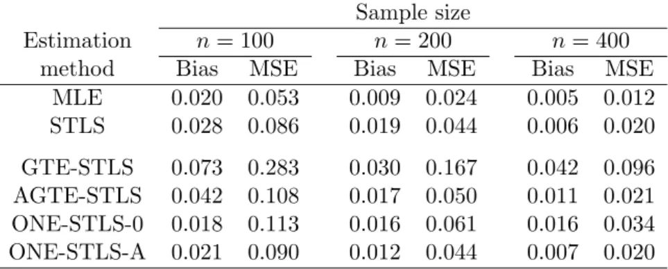
Table 1: The absolute bias and MSE of various estimators for truncated data NORM with n= 100, 200, and 400 observations.
Sample size
Estimation n= 100 n= 200 n= 400
method Bias MSE Bias MSE Bias MSE
MLE 0.020 0.053 0.009 0.024 0.005 0.012 STLS 0.028 0.086 0.019 0.044 0.006 0.020 GTE-STLS 0.073 0.283 0.030 0.167 0.042 0.096 AGTE-STLS 0.042 0.108 0.017 0.050 0.011 0.021 ONE-STLS-0 0.018 0.113 0.016 0.061 0.016 0.034 ONE-STLS-A 0.021 0.090 0.012 0.044 0.007 0.020
Let us note here that we generally look at four types of data containing outlying observations (assuming that l > 1 now): (i) OUT(a; 0,0), where outliers are located at the same place as the remaining observations; (ii) OUT(a;l, l), where outliers are on average at distance
√
2l from the remaining observations, but they are all close to the censoring hyperplane ((1, l, l)>(1,−1,1) = 1); (iii) OUT(a;−l, l), where outliers are on average at distance√2lfrom the remaining observations and they are in the region without (or with a very small number of) censored or truncated observations, at least for larger values of l ((1,−l, l)>(1,−1,1) = 1 + 2l > 0); and (iv) OUT(a;l,−l), where outliers are on average at distance √2l from the remaining observations and they are in the region with many censored or truncated observations, at least for larger values of l((1, l,−l)>(1,−1,1) = 1−2l <0).
To judge the finite-sample behavior of the discussed estimators, we compare different estimators by means of the absolute bias kEβˆn(T)−βk and by means of the squared error
kβˆn(T)−βk2, where ˆβn(T) represents the estimate by a methodT. Because we also analyze the
behavior of all methods in the presence of outliers and the number of simulations is relatively limited (S = 1000), we estimateEβˆn(T) in the absolute bias by meds=1,...,Sβˆn(T,s) and further
report the median squared error (MSE) meds=1,...,Skβˆ(nT,s)−βk2 rather than more usual mean
squared error ( ˆβn(T,s) denotes theT estimate for simulated samples). In some cases, we also
compute the quartiles of the squared error (QSE), which are more informative than just MSE. 5.1 Truncated regression
Let us first discuss the simulation results for the truncated model TM, which are summarized in Tables 1 (data NORM), 2 (data NORM, DEXP, STD(5), HETX, and HETZ), and 3 (data OUTLIER(a;l1, l2)).
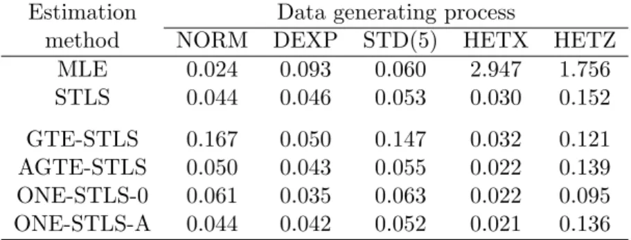
Table 2: The MSE of various estimators for truncated samples without outliers usingn= 200 observations.
Estimation Data generating process
method NORM DEXP STD(5) HETX HETZ
MLE 0.024 0.093 0.060 2.947 1.756 STLS 0.044 0.046 0.053 0.030 0.152 GTE-STLS 0.167 0.050 0.147 0.032 0.121 AGTE-STLS 0.050 0.043 0.055 0.022 0.139 ONE-STLS-0 0.061 0.035 0.063 0.022 0.095 ONE-STLS-A 0.044 0.042 0.052 0.021 0.136
Table 3: The MSE of various estimators for truncated samples with 10% outliers using n= 200 observations.
Estimation Data generating process
method OUT(0.1; 0,0) OUT(0.1; 8,8) OUT(0.1;−8,8) OUT(0.1; 8,−8) MLE (>109,>1010) (14.17, 20.39) (6.385, 10.86) (30.94, 40.32) STLS (0.034, >104) (>102,>105) (>103,>105) (>102,>105) GTE-STLS (0.071, 0.319) (0.077, 0.310) (0.072, 0.331) (0.068, 0.303) AGTE-STLS (0.021, 0.110) (0.028, 0.224) (0.052, 0.730) (0.022, 0.123) ONE-STLS-0 (0.026, 0.134) (0.028, 0.148) (0.080, 0.524) (0.029, 0.133) ONE-STLS-A (0.020, 0.104) (0.027, 0.223) (0.110, 1.130) (0.022, 0.123) In Table 1, we summarize the absolute bias and MSE of all truncated-regression estimators for data NORM and sample sizes n= 100, 200, and 400. As all methods provide consistent estimates and the biases are thus approximately zero, we discuss primarily MSE. Obviously, MLE provides the efficient estimates in this case. The second best estimator is STLS because all other (robust) methods directly or indirectly employ trimming of observations. On one hand, the initial robust estimator, GTE-STLS, exhibits largest bias and MSE of all methods. On the other hand, both AGTE-STLS and ONE-STLS perform significantly better than the initial robust estimator. The ONE-STLS-A actually matches the performance of STLS at all sample sizes and AGTE-STLS does so for n = 400. The relatively worse performance of AGTE-STLS for small samples is likely related to the precision of the residual variance estimate ˆσ0
n, which uses only half of the sample – see (12). Keeping in mind that the relative
performance of AGTE-STLS is worse for n = 100 and better for n = 400, we present the following results only forn= 200.
Next, we compare performance of all methods under various distributional models, see Table 2. Clearly, MLE is no longer the best estimator: it exhibits the largest MSE for data DEXP and it is inconsistent under heteroscedasticity. Similarly, STLS is preferable
only for data NORM and STD(5), but is inferior to the robust estimators in the presence of heteroscedasticity or exponentially distributed errors. Interestingly, GTE-STLS has a large MSE for data NORM and STD(5), but performs well for data DEXP, HETX, and HETZ (in the latest case, it actually outperforms AGTE-STLS). In the cases when GTE-STLS performs well, the ONE-STLS-0 estimator is the best one. In the other two cases, AGTE-STLS and ONE-STLS-A, which have similarly large MSEs, are better than ONE-STLS-0.
Finally, the behavior of all estimator is analyzed for data containing 10% of outliers, data OUT(a;l1, l2) for a = 0.1, lj ∈ {−8,0,8} and j = 1,2 (the results for the contamination levels a = 0.05 and a = 0.20 are very similar). Because the influence of contaminated observations can substantially vary with their precise location and the magnitude of the outlying observations, we report in this case the first and third quartiles of the squared estimation errors (QSEs) instead of MSE, see Table 3. Clearly, both MLE and STLS are in this case extremely influenced by outlying observations irrespective of their location. On the other hand, the most robust GTE-STLS estimator exhibits relatively small QSE, which are stable irrespective of the type of contamination. Other robust alternatives, AGTE-STLS and ONE-STLS, improve upon the initial GTE-STLS estimator except for data OUT(0.1; -8, 8), which contain outlying leverage points in the area with a low truncation probability. The overall best performance can be attributed here to ONE-STLS-0, which is the best of the adaptive and one-step methods for data OUT(0.1; -8, 8) and closely matches the alternatives under other types of contamination.
Altogether, while STLS is sensitive to data contamination, GTE-STLS is robust estimator of truncated regression with very stable, but less precise results across various data-generating models. Considering the adaptive and one-step alternatives, ONE-STLS-0 seems to be the most universal estimator since it performs very well in most of non-Gaussian situations and it stays further behind AGTE-STLS and ONE-STLS-A only for clean Gaussian data. 5.2 Censored regression
Now, we will look at the simulation results for the censored model CM, which are summarized in Tables 4 (data NORM), 5 (data NORM, DEXP, STD(5), HETX, and HETZ), and 6 (data OUTLIER(a;l1, l2)).
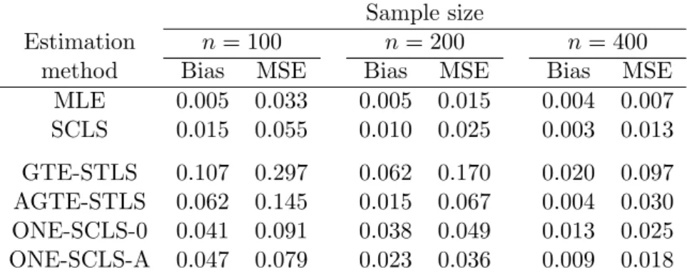
sum-Table 4: The absolute bias and MSE of various estimators for censored data NORM with n= 100, 200, and 400 observations.
Sample size
Estimation n= 100 n= 200 n= 400
method Bias MSE Bias MSE Bias MSE
MLE 0.005 0.033 0.005 0.015 0.004 0.007 SCLS 0.015 0.055 0.010 0.025 0.003 0.013 GTE-STLS 0.107 0.297 0.062 0.170 0.020 0.097 AGTE-STLS 0.062 0.145 0.015 0.067 0.004 0.030 ONE-SCLS-0 0.041 0.091 0.038 0.049 0.013 0.025 ONE-SCLS-A 0.047 0.079 0.023 0.036 0.009 0.018
Table 5: The MSE of various estimators for censored samples without outliers usingn= 200 observations.
Estimation Data generating process
method NORM DEXP STD(5) HETX HETZ
MLE 0.015 0.028 0.024 0.307 0.080 SCLS 0.025 0.038 0.036 0.023 0.111 GTE-STLS 0.169 0.067 0.148 0.033 0.210 AGTE-STLS 0.067 0.059 0.083 0.031 0.237 ONE-SCLS-0 0.049 0.038 0.055 0.023 0.119 ONE-SCLS-A 0.036 0.040 0.050 0.023 0.153
marized for data NORM and sample sizes n = 100, 200, and 400. As all methods provide consistent estimates, the biases are approximately zero. Comparing MSEs, MLE provides the efficient estimates in this case. The second best estimator is SCLS because, similarly to truncated regression, all other (robust) methods directly or indirectly employ trimming of observations. The largest bias and MSE can be attributed to the initial robust estimator GTE-STLS – this comes as no surprise as it uses only half of non-censored observations, that is, about 30–40% observations. On the other hand, both AGTE-STLS and ONE-SCLS perform significantly better than GTE-STLS, with ONE-SCLS-A being best followed by ONE-SCLS-0 and by AGTE-STLS, which uses only non-censored observations and which is thus worst. Note that the MSE of ONE-SCLS-0 (ONE-SCLS-A) is roughly twice (by 38–45%) larger than that of SCLS, but this difference should asymptotically converge to zero (Theo-rem 5). This indicates that using the asymptotic covariance matrix of SCLS with ONE-SCLS in small samples can lead to misleading inference and that bootstrap might be preferable in this situation. Finally, given that these qualitative results do no change much with the sample size, the following results are presented only forn= 200.
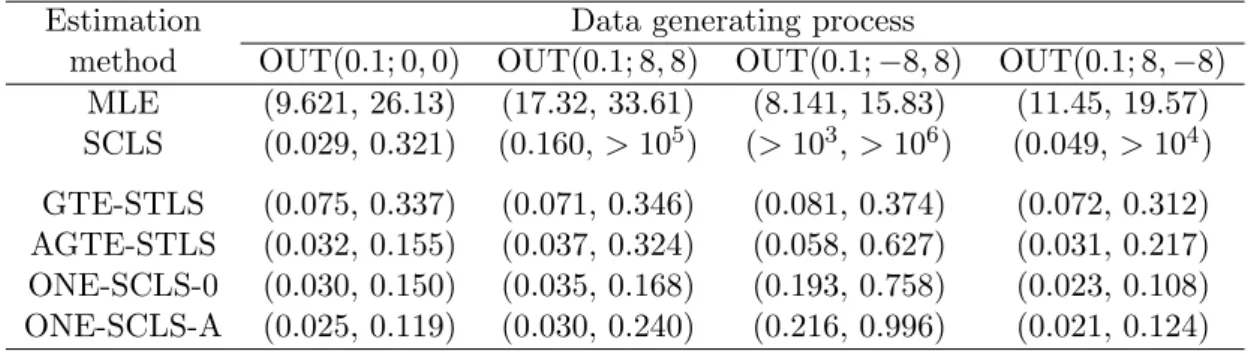
Table 6: The MSE of various estimators for censored samples with 10% outliers usingn= 200 observations.
Estimation Data generating process
method OUT(0.1; 0,0) OUT(0.1; 8,8) OUT(0.1;−8,8) OUT(0.1; 8,−8) MLE (9.621, 26.13) (17.32, 33.61) (8.141, 15.83) (11.45, 19.57) SCLS (0.029, 0.321) (0.160,>105) (>103,>106) (0.049, >104) GTE-STLS (0.075, 0.337) (0.071, 0.346) (0.081, 0.374) (0.072, 0.312) AGTE-STLS (0.032, 0.155) (0.037, 0.324) (0.058, 0.627) (0.031, 0.217) ONE-SCLS-0 (0.030, 0.150) (0.035, 0.168) (0.193, 0.758) (0.023, 0.108) ONE-SCLS-A (0.025, 0.119) (0.030, 0.240) (0.216, 0.996) (0.021, 0.124) Next, we compare performance of all methods under various distributional models, see Table 5. MLE is still the best estimator for models without heteroscedasticity. SCLS is slightly worse than MLE, but it is not biased under heteroscedasticity (data HETX). Let us now consider the robust estimators. Similarly to the truncated-regression case, GTE-STLS has larger MSEs for data NORM and STD(5) and smaller MSEs for data DEXP, HETX, and HETZ relative to other estimators. In the cases when GTE-STLS performs well, the ONE-SCLS-0 estimator matches or outperforms ONE-SCLS-A and AGTE-STLS. On the other hand, ONE-SCLS-A provides practically the best robust estimates except for data HETZ and its MSEs are 0–50% larger than those of SCLS; this difference further reduces to -6–37% forn= 400.
Finally, the behavior of all estimators is analyzed for data containing 10% of outliers, data OUT(a;l1, l2) for a = 0.1, lj ∈ {−8,0,8} and j = 1,2 (the results are qualitatively similar
to those for a= 0.05 anda= 0.20). Because the influence of contaminated observations can substantially vary with their precise location, the magnitude of the outlying observations, and the number of censored and non-censored outliers, we again report the first and third QSE instead of MSE, see Table 6. Clearly, MLE is in this case extremely influenced by outlying observations irrespective of their location. Additionally, SCLS can withstand vertical outliers, data OUT(0.1; 0, 0), but fails in all other data containing outliers (l16= 0 andl2 6= 0). In other
words, SCLS is not influenced by contaminated observations only if they are not outlying in the space of explanatory variables. (The low values of the first QSE in some models is a result of the fact that many outliers can be censored in some simulated data; the estimated median biases of SCLS are however always large: 6–80.) On the other hand, the most robust GTE-STLS estimator exhibits relatively small QSE, which are stable irrespective of the
type of contamination. Similarly to the truncated-regression case, other robust alternatives, AGTE-STLS and ONE-SCLS, improve upon the initial GTE-STLS estimator except for data OUT(0.1; -8, 8). Moreover contrary to MLE and SCLS, all robust estimators exhibit smaller QSE as the sample size increases; for example, the QSE of all robust estimators are 35– 50% smaller for n = 400 than for n = 200 (Table 6). The overall best performance could be probably attributed to ONE-SCLS-0, although the difference between ONE-SCLS-0 and ONE-SCLS-A is not so pronounced as in the truncated case and ONE-SCLS-A becomes preferable with an increasing sample size.
Altogether, SCLS was shown to be sensitive to data contamination, whereas GTE-STLS provided consistent, though less precise estimates across all data-generating models. Select-ing from the adaptive and one-step robust alternatives, ONE-SCLS-A is a preferable robust method in most considered models, especially in models with homoscedastic errors, although it deals quite well also with heteroscedastic and contaminated data in larger samples. How-ever if one believes that data are small, exhibit heteroscedasticity, or contain many outlying observations, ONE-SCLS-0 is a better choice.
6
Conclusion
In this work, we introduced new semiparametric high breakdown-point estimators of trun-cated and censored regression models. Being derived from STLS and SCLS, the estimators are consistent under weak identification assumptions, are asymptotically normally distributed, and additionally, the one-step estimators are asymptotically equivalent to the original STLS and SCLS. Finite sample performance of the proposed robust estimators matches that of STLS in the case of truncated regression. There is a difference in the variance of the ro-bust and SCLS estimates in the case of censored regression, but it is relatively limited even in small samples and more than enough compensated for by the robust properties of the proposed methods.
The robust estimation of truncated and censored regression is studied here only for STLS and SCLS in simple limited-dependent-variable models without, for example, panel-data structures or endogenous regressors. The extension of the GTE and one-step estimation con-cepts to other estimation methods and models is relatively straightforward and can mimic the corresponding extensions of STLS and SCLS, for instance, but remains a topic for further
research.
Appendix
Proof of Theorem 1: Consider a sample Zn= (xi, yi)n
i=1, a constantK >0, and 2p
contami-nated observations (˜xj,y˜j)2j=1p . Forj = 1, . . . ,2p, the contaminated observations (˜xj,y˜j) have
values ˜xj = (1,(−1)jse>[j/2])> and ˜yj = K, where the first element of ˜xj represents the
in-tercept,ej = (0, . . . ,0,1,0, . . . ,0)> denotes thejth basis vector of the Euclidean spaceRp−1,
and s ∈N. Let Zs
n denote the sample created from Zn by replacing its first 2p observation
by data points (˜xj,y˜j)j2p=1 and letµ(Z) =
P
(xi,yi)∈Zyi/|Z|denote the mean of responses in a
sample Z. We now prove that the slopes of the MLE and STLS estimates ˆβ(nM LE−T M)(Zns)
and ˆβn(ST LS)(Zns) in the truncated regression model TM and the MLE and SCLS estimates
ˆ
βn(M LE−CM)(Zns) and ˆβn(SCLS)(Zns) in the censored regression model CM evaluated at the
sequence of samples Zs
n, s ∈ N, converge to 0 as s → ∞ and that the estimated intercepts
converge to +∞.
First, note that the objective functions of all estimators evaluated at βC = (C,0, . . . ,0)
are finite for C ≥ 0 at any Zs
n, s ∈ N, see equations (2)–(5). On the other hand, if we
consider anyβ with nonzero slope coefficients,°°β−(β1,0. . . ,0)>
°
°6= 0,and samplesZs n, the
residuals ˜yj −x˜>j β are equal to K−(−1)jsβ1+[j/2], and consequently, at least one residual
converges to +∞ as s→ ∞ (the residuals yi−x>i β of the remaining observations that are
not contaminated are finite and independent of s). Consequently, the objective function of all estimators converges to +∞ as s→ ∞ for any β with nonzero slope coefficients and the all estimates thus must asymptotically have the form βC = (C,0, . . . ,0) ass→ ∞.
Next, the MLE, STLS, and SCLS estimators at Zs
n reduce thus to the least squares as
s → ∞ if K is sufficiently large because 0 ≤ β>
Cx and yi/2 ≤ βC>x for any x ∈ Rp and
maxi=1,...,nyi/2 ≤ K. These estimates will thus equal βµ = (µ(Zns),0, . . . ,0) at Zns for
s→ ∞. Letting K → +∞ (e.g., by setting K =√s) then results in µ(Zs
n) → +∞ and we
can conclude thatkβˆn(M LE−T M)(Zns)k → ∞,kβˆn(ST LS)(Zns)k → ∞,kβˆn(M LE−CM)(Zns)k → ∞,
and kβˆn(SCLS)(Zns)k → ∞ ass→ ∞ and K→ ∞.
Hence, we have shown that there is a sequence of samplesZns contaminated by 2p obser-vations such that the norms of the MLE, STLS, and SCLS estimators converge to ∞ (and their slopes break down to 0) ass→ ∞irrespective of the initial sampleZn, their breakdown