Information and Search on the Housing Market:
An Agent-based Model
John Mc Breen
∗Florence Goffette-Nagot
†Pablo Jensen
‡ERSA Conference
August 30 - September 3, 2011
Abstract
We simulate a closed rental housing market with search and matching frictions, in which both landlord and tenant agents may be imperfectly informed of the characteristics of the market. The model hypotheses are set so as to match a rent posting search model in the spirit of search models of the labor market. In the simulations, landlords decide what rent to post based on the expected effect of the rent on the time-on-the-market (TOM) required to find a tenant. Each tenant observes their idiosyncratic preference for a random offer and decides whether to accept the offer or continue searching, based on their imperfect knowledge of the distribution of offered rents. The steady state to which the simulation evolves shows price dispersion, nonzero search times and vacancies. We further assess the effects of altering the level of information for landlords. Landlords are better off when they have less information. In that case they underestimate the TOM and so the steady-state of the market moves to higher rents. However, when landlords with different levels of information are present on the market, the better informed are consistently better off. The model setup also allows the analysis of market dynamics. It is observed that dynamic shocks to the discount rate can provoke overshoots in rent adjustments due in part to landlords use of outdated information in their rent posting decision.
1
Introduction
In the urban rental housing market two categories of agents meet. The first category consists of landlords who post rents. The second category consists of tenants who choose among offers. These markets are imperfect as can be seen by the existence of vacancies, price dispersion and nonzero search times for all agents. One source of imperfection is that both categories of agents are imperfectly informed about the characteristics of the market, and acquiring information is costly. These imperfections (in comparison to a theoretical perfectly competitive market) are referred to as search frictions. They have been extensively studied in search-matching models of the labor market, see Rogerson et al. (2005) for a review. Wheaton (1990) created a model of the owner-occupier housing market in which buyers are also sellers and the cost of search effort and its efficiency are defined by an exogenous matching function. This model was later extended to a spatial rental market by Desgranges & Wasmer (2000). The ‘thin’ nature of the housing rental market due to the heterogeneity of housing and tenants’ idiosyncratic tastes has been used to explain vacancies by Arnott (1989).
∗Wageningen University, P.O. Box 9101, 6700 HB Wageningen, The Netherlands. Email:
†Universit´e de Lyon, Universit´e Lyon 2, F - 69007, Lyon, France. CNRS, GATE Lyon-St Etienne, UMR 5824,
69130 Ecully, France. Email: [email protected]
‡ENS-LYON, Laboratoire de Physique, UMR 5672, Lyon, F-69007, France. LET, UMR 5593, Universit´e de
The contribution of the present paper is to propose a multi-agent model as a basis for relaxing many of the assumptions of analytical models in order to obtain a more realistic dynamic model of housing markets. We develop a simulation model of a closed urban hous-ing market focushous-ing on the role of information. In particular, we examine changes in the steady state configuration due to alterations in the level of information available to agents. The major results concern the different influences of the level of information for Landlords. Landlords are penalised when they are better informed, as when they are less well-informed underestimations of the TOM move the market to higher rents which are accepted by the tenants. However, when landlords are heterogeneous in information, the better informed are better off.
It has been shown (Rosen & Smith, 1983) that price dynamics appear to be led by changes in the vacancy rate. More precisely, natural vacancy rates are crucial in determining the strong correlations between fluctuations in the vacancy rate and the evolution of rents. Numerous authors report similar results including Gabriel & Nothaft (1988) also in the rental housing market, Shillinget al.(1987) and Grenadier (1995) in the office rental market and Hwang & Quigley (2006) in the purchasing housing market. In a rental market for single family homes, higher asking rents have been shown to lead to longer TOMs (Allen et al., 2009).
The role of information in the evolution of housing markets has received much attention. Fisheret al.(2003) studied the correlations in prices and liquidity changes over the housing market cycle. Clayton et al. (2008) examined a number of possible explanations of the correlations in price and liquidity changes, and found evidence supporting sellers slow rate for updating their beliefs.
Bradburd et al. (2005, 2006) use agent-based simulations to relax the assumption of a single price with random matching and Nash bargaining in two rental housing models. These static models examine the distributional effects of rent controls (Bradburdet al., 2006) and ‘access discrimination’ (Bradburdet al., 2005), modelled as a reduced matching probability. These analyses however do not explicitly model agents’ search behaviour.
The present paper is organized as follows: section 2 exposes the theoretical hypotheses of an analytical rent posting model; these hypotheses form the basis of the simulated model presented in section 3, the results of which are described in section 4; section 5 concludes.
2
Model
In our rental housing search model, homeless households search for a housing at an acceptable rent. Their reservation rent depends on their idiosyncratic taste which hey discover upon visiting the house. Landlords post rents that become take-it-or-leave-it offers to the tenants. They face a trade-off between setting a higher rent and increasing the probability of finding a tenant. Their optimising behaviour is conditional on the reservation rents of homeless and the rents offered by other landlords. The non-cooperative steady state equilibrium assumes perfect knowledge of other agents’ behaviors and market state.
2.1
Matching function and the vacancy/homeless rate
There is a continuum of households an a continuum of landlords, each of measure 1. The numbers of vacant housing and homeless individuals are respectively writtenvandh. Search-ing households and owners of unoccupied housSearch-ings meet at each period followSearch-ing a matchSearch-ing function: m=m(v, h). This matching function is supposed homogenous of degree one, in-creasing and concave in its two arguments. As a consequence, the probability for a landlord to meet a searching tenant is:
m(h, v) v =m h v,1 =m 1 θ,1 ≡q(θ) (1)
with θ≡v/hthe housing market tightness, that is the number of vacant housing units per homeless individual.
Similarly, the arrival rate of housing opportunities to homeless individuals is: m(h, v) h =m 1,v h =m(1, θ) =θq(θ) (2)
Landlords incur a maintenance cost for having their housing on the market, be it occupied or vacant. They can withdraw from the market of the value of having it on the market is below the maintenance cost. As each landlord owns only one housing unit, the number of vacant housing units varies only due to the withdrawal of units from the market.
2.2
Tenants’ stopping rule
Each tenant has an incomey that is drawn from a uniform distribution in the range [y;y]. Tenant agents have a separable utility function whose housing part differs depending on their situation on the housing market (housed or searching). There is an heterogeneity in the utility procured by the matching of a tenant and a housing unit: agents have an idiosyncratic preference for an apartment, that is discovered by the agent once the apartment is visited. Therefore, when housed, the agent’s instantaneous utility flow from ‘housing’ is given by:
Uh=y−r+η (3)
where Uh is the instantaneous utility flow, y is housing budget, r is the rent paid and η is the idiosyncratic preference of an agent for an apartment1. η ∼N(0, σ), whereσ is the
variance of the normally distributed idiosyncratic preferences. While searching, the agent’s instantaneous utility flow from ‘housing’ is Us =y−c where c is the monetarised cost of searching.
At each period, with a certain probabilityλ, a searching agent sees one randomly chosen apartment from the distribution of offers and decides whether to accept it or keep searching. Decisions are made based on an optimising behaviour that trade-offs a quicker match, and therefore reduced search costs, against a lower rent. This optimsing behavior is based on the knowledge of the rent offer distribution and the distribution of idiosyncratic tastes. This is summarized in the choice of a reservation utility, the minimum utility an agent is willing to accept from a residence. This reservation utility determines, once the match quality η is known, the reservation rentr∗(η) as a function ofη.
The tenant stopping rule is based on the writing of the continuous time Bellman equations for housed and non housed tenants. The value of a searching agent V0(y) depends on the
agents’ income. The value of a housed tenantV1(r, η, y) is affected by her current rent and
match quality, as well as her income. At steady state, the value of a tenant who pays rentr and occupies an apartment with match quality η is such that:
τ V1(r, η, y) =y−r+η+δ(V0(y)−V1(r, η, y)) (4)
with δ the exogenous probability of leaving at each period. This equation shows that the instantaneous return from being housed withr andη is the instantaneous utility from this state plus the benefit (or more precisely loss) that would ensues from leaving this situation, which occurs with probability δ.
The value of searching for a non-housed tenant is such that: τ V0(y) =y−c+λ Z η " Z r∗(η) −∞ (V1(y, r, η)−V0(y))dF(r) # dΦ(η) (5)
withF the cumulative distribution function of rents andH that of η.
Equation 4 allows to write the difference between the value of housed tenants paying rent rwith match qualityη and the value of homeless tenants, with respect toV0. Inserting this
expression in equation 5 gives: τ V0(y) =y−c+ λ τ+δ Z η " Z r∗(η) −∞ (y−r+η−τ V0(y))dF(r) # φ(η)dη (6) The reservation rent is the rentr∗(η) that verifies:
V1(y, r∗(η), η) =V0(y) (7)
1
This parameter can be understood as a distance between the agent and the apartment characteristics, in a context of horizontal differenciation.
which, given equation 4 implies:
τ V0(y) =y−r∗(η) +η (8)
Inserting this expression in equation 6 gives: τ V0(y) =y−c+ λ τ+δ Z η " Z r∗(η) −∞ (r∗(η)−r)dF(r) # φ(η)dη (9) and finally: r∗(η) =η+c− λ τ+δ Z η " Z r∗(η) −∞ (r∗(η)−r)dF(r) # φ(η)dη (10)
withφthe probability density function ofη. In the following, we will note k≡λR η h Rr∗(η) −∞ (r ∗(η)−r)dF(r)iφ(η)dη.
Equation 10 highlights that a distribution of reservation rents exists due to the distri-bution of idiosyncratic tastes. In other words, the reservation utility level is common to all searching agents, while reservation rents are determined as the difference between this reser-vation utility and the idiosyncratic taste discovered upon visiting the apartment. Accepted rents will then depend on the distribution of η. The cumulative distribution function of η will of be noted Φ(.) in the following.
2.3
Landlords’ behavior
Landlords have three possible states: having a tenant at rent r, being on the market and being off the market. The corresponding instantaneous profits are: πo(r) =r−mthe rent minus the maintenance cost,πv(r) =−m, and 0 their outside profit.
Landlords behave by maximizing the sum of expected net benefits they have from putting their housing unit on the market. Rents are set so as to maximize the return of doing so. Landlords know the distribution of accepted rents and of of rents offered by other landlords. Therefore in particular, they never set a rent higher than the homeless costc, nor do they put a rent lower than their maintenance costm.
The Bellman equation for a landlord putting her apartment on the market is: τ W0= max
m≤r≤c{−m+P(r)q(θ)(W1(r)−W0(r))} (11) with m the maintenance cost of a vacant housing on the market, q(θ) the probability to meet a searching tenant and P(r) the probability that rent r is accepted by the searcher, which depends on the distribution of the match quality and reservation rentr∗(η). In words,
the expected net return of holding a vacant housing on the market equals the product of the rate at which searching tenants are metq(θ), the probability for the encountered tenant to accept the offered rent and the capital gain of having a tenant paying rent r, minus the maintenance cost of the vacant housing.
The Bellman equation for a landlord renting her apartment at rentr solves:
τ W1(r) =−m+r+δ(W0−W1(r)) (12)
In words, the expected net return of holding a housing rented at rent r equals the instan-taneous payoff minus the maintenance cost of the housing, plus the product of the rate at which tenants leave and the capital gain of having a tenant paying rentr.
Combining the two Bellman equations yields:
τ W0=−m+P(r)q(θ) r
3
Agent based model
The simulated model mimics the theoretical hypotheses presented above, although the inter-actions between agents do not result from equilibrium hypotheses but from “real” interinter-actions between the simulated agents.
3.1
Agents’ behavior
Tenantsare supposed to observe a sample of the offer distribution and to visit one randomly chosen residence each iteration. They accept offers based on an optimising behaviour that trade-offs a quicker match, and therefore reduced search costs, against a lower rent. Tenants must decide their reservation utilityUres, the minimum utility they are willing to accept from a residence. They obtain a utility flow Uh from the market, after experiencing a negative utility flow UT
s while searching. Tenant agents’ have a separable utility function whose housing part differs depending on their situation on the housing market. When housed, the agent’s instantaneous utility flow from ‘housing’ is given by: UT
h = Y −R+η ≥0 where UT
h is the instantaneous utility flow, Y is housing budget, R is the rent paid and η is the idiosyncratic preference of an agent for an apartment that is discovered by the agent once the apartment is visited. η ∼N(0, σ), where σis the variance of the normally distributed idiosyncratic preferences. σ is a percentage of the housing budget, see Table 1. While searching, the agent’s instantaneous utility flow from ‘housing’ isUT
s =Y −CT <0 where CT is the monetarised cost of searching.
Each tenant has a housing budget Y that is drawn from a uniform distribution in the range [100,198]. A searching agent sees one randomly chosen apartment from the distribution of offers and must decide whether to accept it or keep searching. This will depend upon their idiosyncratic preference for the apartment, the posted rent, their housing budget, the cost of search and their outside opportunity, that is, the value of continuing to search, which they assess based on their knowledge of the distribution of apartements’ characteristics that determine the idiosyncratic taste for the apartments and of a percentage ST of the full distribution of offers.
Ures is optimised to yield the maximum utility per unit time over the expected period of search and residence. Tenant agents idiosyncratic preferences do not play a role in this decision.
The expected benefit per unit time for a given reservation utility is given by:
BT(Ures) = UT s X+T(Ures) T(Ures) Z 0 exp(τ t)dt+ E UT h X+T(Ures) T(Ures)+X Z T(Ures) exp(τ t)dt (14) whereUT
s is the utility flow experienced while searching,X is the expected duration of residence, T(Ures) is the expected search time, τ is the discount rate and E
UT
h
is the expected utility flow per iteration once housed if the chosen reservation utility isUres.
Equation (14) is rewritten: BT(Ures) = UT s X+T(Ures) [1−exp (−τ T(Ures))] + E UT h X+T(Ures)
[exp (−τ T(Ures))∗(1−exp (−τ X))]. (15) The first line in Equations (14) & (15) are the total expected discounted search cost di-vided by the full expected duration of search and residency. The second line is the discounted total expected utility flow during residency divided by the full expected duration of search and residency. Equation (14) is similar to that used by Igarashi (1991) for the expected discounted housing costs of a searcher. This equation differs from it however, as here we take the expected benefit per unit time. Also, for the sake of simplicity, we do not explic-itly include in the agents’ optimization the discounted expected benefit upon re-entering the
market after the tenant eventually leaves the residence. This choice does not impact the qualitative results of the model in a context where agents assume the market state to be constant.
Whenτ, the discount rate is zero, equation (14) can be simply written: BT(Ures) = UT s X+T(Ures) T(Ures) + E UT h (Ures) X+T(Ures) X (16)
This equation is included as it is the reference simulation, and is easier to interpret. The expected search timeT(Ures) is equal to the number of residences seen divided by the number of acceptable residences. E
UT h (Ures)
is given by the average utility of residences, which are expected to yield utilities larger thanUres. Once a residence is rejected it cannot be revisited, unless it remains vacant and is randomly reselected. All tenant agents participate in the housing market and searching tenant agents recalculate their reservation utility each iteration.
Landlordshave three possible states, having a tenant, being on the market and being off the market. The corresponding utilities are,UL
occ=R−CL the rent minus the maintenance cost,UL
vac=−CL, and 0 their outside opportunity.
Landlords’ decision variable is what rent to post. In making this decision, they are assumed to trade-off speed of sale with rent procured. Landlords calculate their most advan-tageous rent, that is the rent that in expectation provides the highest benefit per iteration, given that contracts are for fixed rents and have an exogenous probability 1/X of being terminated each iteration.
The function that gives this expected benefit isBL(R) :
BL(R) = −CL X+T(R) Z T(R) 0 e−τ tdt+ R−CL X+T(R) Z X+T(R) T(R) e−τ tdt (17) where τ f is the discount rate, X is the exogenous expected time a tenant will stay in the apartment,CLis the maintenance cost per iteration andT(R) is the expected time-on-the-market, whose calculation is described below.
Equation 17 is rewritten: BL(R) = −CL X+T(R)[1−exp (−τ T(R))] + R−CL X+T(R)[exp (−τ T(R))∗(1−exp (−τ X))]. (18) The first line in Equations (17) & (18) is the total expected discounted costs incurred while searching for a tenant, divided by the full expected time-on-the-market and residency duration. The second term is the total expected discounted utility flow during occupancy, divided by the full expected time-on-the-market and residency duration. Note that the overall time over which the profit is determined varies withT(R). Average landlord welfare is the average utility over all landlords.
When the discount rateτ is zero, equation 17 can be written: BL(R) =
−CL
X+T(R)T(R) +
R−CL
X+T(R)X (19)
Landlords’ optimising behaviour is based on their knowledge of the market state, in terms of TOM for different asking rents. They must estimate the relationship between TOM and expected rent flows. They are assumed to have access to information on a certain percentage of residences on the market over the last F iterations. They know for these residences, how many iterations they were on the market at their most recent market price, within the lastF iterations. They also know whether or not they have been rented, as shown in Figure 1. The above procedure generates two histograms, one of the cumulative times on the market within each rent interval, and one of the number of sales within each interval. This allows landlords to calculate the probability per iteration of finding a tenant for a range of rent intervals,
now not counted rent change counted rented put on market F t
Figure 1: The periods of time-on-the-market known to landlords.
implicitly assuming that the probability to sell was constant. This probability is simply the number of agreed rents divided by the cumulative times on the market. The landlords estimate the best least-squares fit of the exponential function for the expected TOM T(R) as a function of the rentR.2 3 T(R) =αexp(βR), whereαandβ are fit parameters. Figure
2 shows an example fit ofT(R) and the corresponding expected profits. Landlords review their decisions with probability 1/F.
100 105 110 115 120 125 130 135 Posted Rent 0 20 40 60 80 100 120 140 160 Expected TOM Observations Exponential Fit 100 105 110 115 120 125 130 135 Posted Rent -40 -30 -20 -10 0 10
Expected gain per iteration
❘
^
Figure 2:
Left
: Example of an estimated relation (red line) between asking rent and TOM per
rental. The size of the ‘error bars’ is the statistical weight given to each point in the least-squares
fit of the exponential.
Right
: The corresponding expected profits.
3.2
Simulation procedure
• Searchers visit a randomly chosen apartment, and accept or reject it.
• A portion of landlords (1/F) whose apartments remain vacant decide if they shall change their rent or withdraw from the market.
• A portion of landlords (1/F) who have withdrawn from the market decide if they shall return.
• A certain fraction (1/X) of tenants, randomly chosen, leave. • Landlords of newly empty apartments choose their asking rents. • The next iteration begins.
In Table 1 the parameters of the model are listed, these are used in all results presented, unless stated otherwise. Analysis of the model’s behaviour under variations in these param-eters can be found in Mc Breen et al. (2009). The default value of X is assumed to be 4 years (see de Una-Alvarezet al. (2009)), meaning thatF is three months.
2
Each pointT(R) =ωis given a weight equal to the natural logarithm of the number of rentalsN(R) in the rent interval centered onR, plus one, that isweight= ln (N(R) + 1).
3
Table 1: Parameters of the Simulation Model
Symbol Meaning Default Value of Parameters
Landlords’ parameters
CL Maintenance cost 100
SL % of sales seen 20%
F Timescale rent changes (and memory) (iterations) 15
RI Estimation rent interval size 2
Tenants’ parameters
Y Housing budget [100-198]
CT Search costs 200
ST Percentage of offers seen 5%
X Expected length of residence (iterations) 240 σ Idiosyncrasy of tenants preferences (%Y) 5
General parameters τ Discount rate
size Number of households 10000
Z Number of initializing iterations 10
0 500 1000 1500 2000 Iterations 0 2000 4000 6000 8000 10000 Population
Pop: High initial rents Pop: Low initial rents
0 500 1000 1500 20000 20 40 60 80 100 Off-market landlords
Off-market: Low init rents Off-market: High init rents
100 120 140 Rents 0 100 200 300 400 500 Rents posted Rents accepted
Figure 3:
Left
: The steady state population and number of landlords off-the-market.
Right
:
Rents posted and accepted in last 15 iterations at the steady state, after 2000 iterations.
4
Results
As can be seen in Figure 3-Left, the basic model converges for any initialization to a rea-sonable steady-state with a positive vacancy rate, rent dispersion and nonzero search times. The dispersion in both accepted and posted rents can be seen in Figure 3-Right. We see that most landlords offer rents close to the ‘going rate’. The few who ask higher rents are less likely to find tenants. As in existing analytical models, the heterogeneity of tenants’ in-comes and the presence of market frictions contribute to the dispersion of rents. Additional factors contributing to the dispersion of prices are the idiosyncratic preferences of tenants and stochastic information effects: agents observe different samples of market signals and therefore take different decisions.
4.1
Landlords’ Information Level
Landlords’ Information Levels, SL were varied for both homogeneous and heterogeneous landlord populations. Increasing homogeneous landlords’ information decreases rents, Figure 4-Left. Landlords need accurate two dimensional information, that is rents offered and their associated times-on-the-market to make good decisions. Their information on TOM for different rents is based on a finite sample accumulated over F iterations. The
over-0 10 20 30 40 0 50 100 150 200 TOM TOM 0 10 20 30 40 Landlords’ information (%) 120 125 130 135 140 145 150 Rent Average Rent 0 20 40 60 80 100 % landlords with SL = 5% 0 10 20 30 40 50 60 70 TOM TOM 0 20 40 60 80 100 125 130 135 140 Rent Average Rent
Figure 4:
Left
: The average rent and the average TOM for homogeneous landlords.
Right
: The
average rent and the average TOM as a function of the percentage of landlords who see 5% of
the available information while all other landlords see 20%.
0 20 40 60 80 100 % landlords with SL = 5% 10 15 20 25 30
Welfare Average tenant welfare
Average landlord welfare : SL = 5%
Average landlord welfare : SL = 20%
Figure 5: The average welfares (current utility flows) of tenants and both types of landlord as a
function of the percentage of landlords who see 5% of the available information while all other
landlords see 20%.
estimations of the optimal rent of less informed landlords result from their underestimation of TOM. Ill-informed landlords are less likely to see the long waiting times (TOM) for very high rents which are rarely accepted. This leads to higher asking rents. As the landlords are homogeneous, and make the same errors on average, this pushes the market rents upwards. Every high posted rent, if refused by tenants, increases their expected search times as tenants’ search is undirected. This necessarily affects searchers’ optimal reservation utilities, pushing the market towards higher rents. In contrast, increasing landlords’ information makes them sharper competitors, leading to reduced rents.
In order to further test the effect of landlords’ information on the steady-state of the market we perform simulations with landlords who areheterogeneous in information. There are two types of landlord, those with the default level of information SL = 20 and those with SL = 5, values that were chosen because Figure 4-Left shows that the steady state changes significantly between these two values when they are shared by all landlords. Figure 4-Rightshows the increases in average rents and times-on-the-market with the proportion of ill-informed landlords. This is because errors made by ill-informed landlords tend to lead to higher rents. This changes the distribution seen by tenants who have no option but to lower their reservation utilities. As a consequence, well-informed landlords react to the reduced TOM for a given rent by increasing their asking rents as well.
In Figure 5 we see that, due to the increase in rents, the welfare of both types of landlords increases as the proportion of ill-informed landlords rises. However, the better informed always have higher welfares. This results from their more accurate appreciation of the state of the market. In summary, there are positive externalities (or, more precisely, market effects) of ill-informed on well-informed landlords, the former moving the market rent upwards.
0 2 4 6 8 10 12 14 20 22 24 26 28 30 32 34 36 TOM TOM 0 2 4 6 8 10 12 14
τ −
discount rate
120 122 124 126 128 130 Rent Average rent 0 2 4 6 8 10 12 14 τ - Discount rate 15 20 25 30 WelfareAverage tenant welfare Average landlord welfare
Figure 6:
Left
:The average rent and the average time-on-the-market for residences rented over
the last 15 iterations.
Right
: The average welfares of tenant and landlord agents. Both graphs
for a variation in the annual discount rate of both agent types.
4.2
Dynamically varying the discount rate
The discount rate incorporates the value of time, represented by the real interest rate.4
The discount rate was varied from less than 1% per annum to over 17% per annum. Increasing the discount rate means an increase in the impatience of all agents. That is, at constant rents and TOM, for both categories of agent the value of a match increases with respect to the value of continuing to search. More specifically, changing the discount rate alters all four terms in the right-hand sides of Equations 14 & 17.
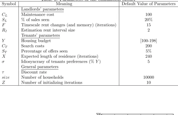
There ensues two contradictory effects: Landlords have a tendency to post lower rents, while tenants are willing to accept higher rents, conditionally on their income. It is not obvious which of these effects should dominate. In general, one may anticipate that the effects of changes in the discount rate depend on the relative influence of tenants and landlords in the market. As landlords post prices which cannot be negotiated, while tenants decide whether or not to accept the offer received, we can expect landlords’ decisions to lead the market.
Figure 6-Left shows that for the default values of the other parameters, the average rent is lower with a higher discount rate. This shows that changes in landlords’ behaviour, due to a change in discount rate, have a greater impact on market outcomes than the corresponding changes in tenants’ behaviour. Increases in the discount rate also lead to a reduction in TOM and an increase in population. Therefore, the average welfare of tenants is improved and that of landlords disimproved with increasing discount rates, as can be seen in Figure 6-Right .
The role of information in the context of a dynamic evolution of real estate markets is an important subject that has already been analysed empirically by Fisher et al. (2003); Clayton et al. (2008). In order to examine this question we introduce exogenous shocks to the discount rate. Two aspects of information play an important role in the decisions of landlords: Firstly the proportion of available information seen and secondly the length of their memory. At the steady state, these two parameters have an equivalent role: both increase the quantity (and therefore quality) of information. However, in an evolving market, the length of memory becomes a two-edged sword. It increases the quantity of information but much of this information may be out-of-date.
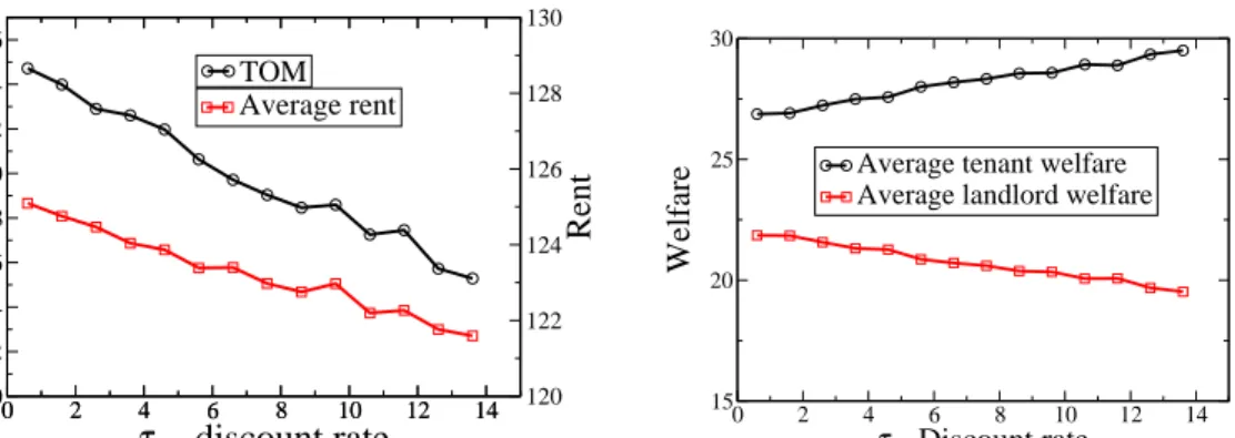
The discount rate was varied from 2% to 10% at 1500 iterations and reduced again to 2% at 3000 iterations. The adjustments in the rent and the TOM due to the changes in the discount rate can be seen in Figure 7-Right. As expected from the comparative statics shown in the previous subsection, both the average rent and TOM reduce after the increase in the discount rate. This causes an increase in population due to the larger number of tenants who 4
1000 2000 3000 4000 Iteration 8300 8400 8500 8600 8700 8800 8900 9000 9100 9200 9300 Population Population 1000 2000 3000 4000 Iteration 0 500 1000 1500 2000 Off-market / Vacant Vacant Off-market 1000 2000 3000 4000
Iteration
0 10 20 30 40 50 60TOM
TOM 1000 2000 3000 4000Iteration
115 120 125 130 135 140 145TOM
Average rentFigure 7:
Left
: The variations in population, vacancies and the number of landlords off the
market, with the varying discount rate
r
shown
Right
.
Right
: The exogenous variation of the
discount rate and the corresponding average TOM.
1500 1600 1700 1800 1900
Iteration
0 10 20 30 40 50TOM
TOM 1500 1600 1700 1800 1900Iteration
120 125 130Average rent
Average rent 3000 3100 3200 3300 3400Iteration
0 10 20 30 40 50 60TOM
TOM 3000 3100 3200 3300 3400Iteration
122 124 126 128 130 132Average rent
Average rentFigure 8:
Left
: The variations in TOM and average rents, around the transition of the discount
rate from
τ
= 2% to
τ
= 10% at 1000 iterations.
Right
: The variations in TOM and average
rents, around the transition of the discount rate from
τ
= 10% to
τ
= 2% at 2000 iterations.
can afford housing (see Figure 7-Left). Opposing adjustments occur when the discount rate comes back to its previous value. This gives us the opportunity of exploring the dynamics of the market in situations of both rising prices and falling prices.
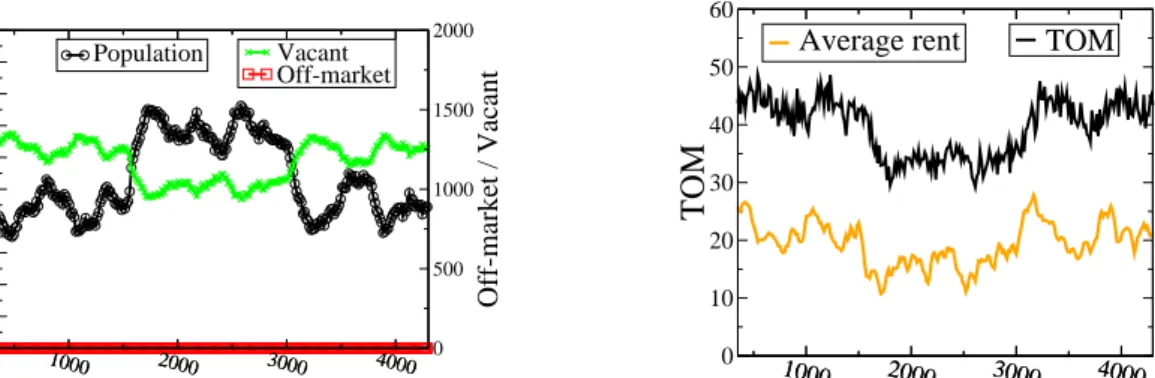
All landlords who review their rent after the increase at 1500 iterations are aware of the increase in the discount rate, and therefore post lower rents. Their beliefs on the state of the market evolve more slowly due to their memory of past transactions. Therefore, as tenants’ reactions to the new situation are not taken into account immediately, accepted rents reduce abruptly, see Figure 8-Left.
However, the average TOM of agreed rents reduces considerably more slowly. Tenants change immediately their reservation utility in reaction to the flow of new low rents. There-fore the average individual acceptance probability reduces due to newly increased value of waiting for these particularly low rents. This hinders the decrease in TOM that would oth-erwise result from the greater number of tenant agents who can afford housing. Once the rent distribution stabilises, that is the newly posted rents cease to be cheaper than those on the market, average individual acceptation probabilities increase. We observe in Figure 8-Left that just before the average TOM reaches its new steady-state value the rent is at its lowest level. Coupled with the greater number of tenant agents who can now afford housing, this causes the volume and population to rise until the new steady-state is reached. Figure 9-Left shows that the population rises by approximately 250 in 200 iterations, equivalent to about 21
2 years. As the number of departures is a constant fraction of the population, at
1500 1600 1700 1800 1900 Iteration 8400 8600 8800 9000 9200 Population Population 1500 1600 1700 1800 1900 Iteration 0 500 1000 1500 2000 Off-market / Vacant Vacant Off-market 3000 3100 3200 3300 3400 Iteration 8400 8600 8800 9000 9200 Population Population 3000 3100 3200 3300 3400 Iteration 0 500 1000 1500 2000 Off-market / Vacant Vacant Off-market
Figure 9:
Left
: The variations in population, vacancies and the number of landlords off the
market, around the transition of the discount rate from
τ
= 2% to
τ
= 10% at 1000 iterations.
Right
: The variations in population,vacancies and the number of landlords off the market,
around the transition of the discount rate from
τ
= 10% to
τ
= 2% at 2000 iterations.
population is rising the volume of transactions is greater than at a steady-state with the same population. Once the rents have ceased to reduce the volume of transactions increases for a short period, around 1570 iterations, as seen by the sharp rise in the population in Figure 9-Left. In fact the volume of transactions increases by over 15% temporarily before lowering to its steady state value that, like the new population, is approximately 3% above its previous steady-state value. The higher volume of transactions in conjunction with a smaller number of vacancies at the new steady-state keep TOM low.5 Changes in the ratio
of transaction volumes to vacancies are an essential element that differentiate ‘hot’ and ‘cold’ markets.
After the reduction in the discount rate at 3000 iterations opposite adjustments are seen: an increase in average rent, TOM and the vacancy rate with a decrease in population. A decrease in volume follows from the falling population seen in Figure 9-Right. The rent increases immediately as landlords are instantly informed of the reduction in the discount rate, see Figure 8-Right. What’s new here is first that the population falls immediately with the increase in rent as poorer tenants have a hard income constraint, see Figure 9-Right.
Secondly, there is a marked overshoot in rents, see Figure 8-Right. This can be attributed to the fact that the eventual negative effects of asking excessive rents take time to be under-stood by landlords. This is due to both the low frequency of acceptation of high rents, which means that they are often unobserved by individual landlords, and secondarily the relatively long time required for these durations to happen.
5
The average TOM for landlords is proportional to the number of vacancies divided by the volume of transac-tions in an iteration. Here, the change in TOM is primarily due to the change in the number of vacancies, which changes by around 20% rather than to the 3% change in volume.
5
Conclusion
Our dynamic model includes imperfect information and heterogeneous interacting agents. It leads to price dispersion, nonzero search times and vacancies, three essential ingredients of any realistic housing model. The matching probability depends endogenously on the posted price of apartments.
The heuristics of real world landlords are simulated here by a regression and profit calcu-lation, with a larger number of individual information points than real agents normally know. In our model landlords set rents which tenant agents accept or refuse. Greater information for landlords disimproves their overall utility due to greater competition. However, when landlords with different levels of information are present on the market, the better informed are consistently better off.
We have examined the comparative static and dynamic effects of a change in the discount rate. Landlords have greater market power as they set the rents among which agents choose. It has been shown that rents are lower with higher discount rates, as landlords cost of search out-weighs the gain from higher rents. There is evidence of overshooting in the adjustment of rents after shocks.
Our main aim has been to construct a model that allows hypotheses on the functioning of the urban rental market to be investigated. We believe that a dynamic model based on straightforward micro-economic behaviours with imperfect information is a good approach. We have found robust and simple agent dynamics (or rules) that reproduce important features of the rental housing market.
The current set-up allows the investigation of the distributive effects of policy decisions among tenant agents of varying incomes. Rent control is one possible example Bradburd et al.(2006), as is the level of information among tenants Bradburdet al.(2005).
The agent-based approach adopted here allows many sources of heterogeneities, that can-not be modelled analytically, to be included. It also has considerable potential for modelling the dynamics of housing markets.
References
Allen, M.T., Rutherford, R.C., & T.A., Thomson. 2009. Residential Asking Rents and Time on the Market. Journal of Real Estate Finance and Economics,38(4), 351–365.
Arnott, R. 1989. Housing vacancies, thin markets, and idiosyncratic tastes. Journal of Real Estate Finance and Economics, 2, 5–30.
Bradburd, R., Sheppard, S., Bergeron, J., Engler, E., & Gee, E. 2005. The distributional im-pact of housing discrimination in a non-Walrasian setting.Journal of Housing Economics, 14(2), 61–91.
Bradburd, R., Sheppard, S., Bergeron, J., & Engler, E. 2006. The impact of rent controls in non-Walrasian markets: An agent-based modeling approach.Journal of Regional Science, 46(3), 455–491.
Clayton, J., MacKinnon, G., & Peng, L. 2008. Time variation of liquidity in the private real estate market: An empirical investigation. Journal of Real Estate Research, 30(2), 125–160.
de Una-Alvarez, Jacobo, Arevalo-Tome, Raquel, & Soledad Otero-Giraldez, M. 2009. Non-parametric Estimation of Households’ Duration of Residence from Panel Data. Journal Of Real Estate Finance And Economics,39(1), 58–73.
Desgranges, G., & Wasmer, E. 2000. Appariements sur le marche du logement. Annales d’economie et de statistique, 253–287.
Fisher, J., Gatzlaff, D., Geltner, D., & Haurin, D. 2003. Controlling for the impact of variable liquidity in commercial real estate price indices. Real Estate Economics,31(2), 269–303. Gabriel, S.A., & Nothaft, F.E. 1988. Rental housing markets and the natural vacancy rate.
American Real Estate and Urban Economics Association Journal,16(4), 419–429. Grenadier, SR. 1995. Local And National Determinants Of Office Vacancies. journal Of
Urban Economics,37(1), 57–71.
Hwang, M., & Quigley, J.M. 2006. Economic fundamentals in local housing markets: Evi-dence from US metropolitan regions. Journal of Regional Science,46(3), 425–453. Igarashi, M. 1991. The rent-vacancy relationship in the rental housing market. Journal of
Housing Economics,1, 251–270.
Mc Breen, J., Goffette-Nagot, F., & Jensen, P. 2009. An Agent-Based Simulation of Rental Housing Markets.
Rogerson, R., Shimer, R., & Wright, R. 2005. Search theoretic models of the labour market: A survey. Journal of Economic Literature,63, 959–988.
Rosen, K.T., & Smith, L.B. 1983. The price-adjustment process for rental housing and the natural vacancy rate. American Economic Review,73(4), 779–786.
Shilling, J.D., Sirmans, C.F., & Corgel, J.B. 1987. Price adjustment process for rental office space. Journal of Urban Economics, 22(1), 90–100.
Wheaton, W.C. 1990. Vacancy, search, and prices in a housing market matching model. Journal of Political Economy,98(6), 1270–1292.
Appendix: Simulation initialisation phase
The landlords all have an initial asking rent randomly chosen in the interval 100-120. The tenant agents have a uniform distribution of housing budgets between 100 and 198 in 50 discrete groups. Over the first Z iterations, tenant agents see five apartments and select the lowest asking rent if it offers the agent a positive utility. This preference for lower rent residences initialises the market in such a way that the information available to landlords indicates that higher rents mean longer waiting times. Landlords do not review their rents during the initialisation phase. After theZ initialisation iterations are complete, the mech-anism described in the body of the text is implemented, in which searchers see only one residence per iteration.