Evaluating techniques for mapping island vegetation from unmanned aerial vehicle (UAV) images: Pixel classification, visual interpretation and machine learning approaches

(1)

Research Online

Faculty of Science, Medicine and Health -

Papers: Part B

Faculty of Science, Medicine and Health

1-1-2020

Evaluating techniques for mapping island vegetation from

unmanned aerial vehicle (UAV) images: Pixel classification, visual

interpretation and machine learning approaches

Sarah Hamylton

University of Wollongong, [email protected]

Rowena H. Morris

University of Wollongong, [email protected]

Rafael Cabral Carvalho

University of Wollongong, [email protected]

N Roder

University of Wollongong

P Barlow

University of Wollongong

See next page for additional authors

Follow this and additional works at: https://ro.uow.edu.au/smhpapers1

Publication Details Citation

Hamylton, S., Morris, R. H., Cabral Carvalho, R., Roder, N., Barlow, P., Mills, K., & Wang, L. (2020). Evaluating

techniques for mapping island vegetation from unmanned aerial vehicle (UAV) images: Pixel

classification, visual interpretation and machine learning approaches. Faculty of Science, Medicine and

Health - Papers: Part B. Retrieved from https://ro.uow.edu.au/smhpapers1/1327

Research Online is the open access institutional repository for the University of Wollongong. For further information

contact the UOW Library: [email protected]

(2)

vehicle (UAV) images: Pixel classification, visual interpretation and machine

learning approaches

Abstract

We evaluate three approaches to mapping vegetation using images collected by an unmanned aerial

vehicle (UAV) to monitor rehabilitation activities in the Five Islands Nature Reserve, Wollongong

(Australia). Between April 2017 and July 2018, four aerial surveys of Big Island were undertaken to map

changes to island vegetation following helicopter herbicide sprays to eradicate weeds, including the

creeper Coastal Morning Glory (Ipomoea cairica) and Kikuyu Grass (Cenchrus clandestinus). The spraying

was followed by a large scale planting campaign to introduce native plants, such as tussocks of

Spiny-headed Mat-rush (Lomandra longifolia). Three approaches to mapping vegetation were evaluated,

including: (i) a pixel-based image classification algorithm applied to the composite spectral wavebands of

the images collected, (ii) manual digitisation of vegetation directly from images based on visual

interpretation, and (iii) the application of a machine learning algorithm, LeNet, based on a deep learning

convolutional neural network (CNN) for detecting planted Lomandra tussocks. The uncertainty of each

approach was assessed via comparison against an independently collected field dataset. Each of the

vegetation mapping approaches had a comparable accuracy; for a selected weed management and

planting area, the overall accuracies were 82 %, 91 % and 85 % respectively for the pixel based image

classification, the visual interpretation / digitisation and the CNN machine learning algorithm. At the scale

of the whole island, statistically significant differences in the performance of the three approaches to

mapping Lomandra plants were detected via ANOVA. The manual digitisation took a longer time to

perform than others. The three approaches resulted in markedly different vegetation maps characterised

by different digital data formats, which offered fundamentally different types of information on vegetation

character. We draw attention to the need to consider how different digital map products will be used for

vegetation management (e.g. monitoring the health individual species or a broader profile of the

community). Where individual plants are to be monitored over time, a feature-based approach that

represents plants as vector points is appropriate. The CNN approach emerged as a promising technique

in this regard as it leveraged spatial information from the UAV images within the architecture of the

learning framework by enforcing a local connectivity pattern between neurons of adjacent layers to

incorporate the spatial relationships between features that comprised the shape of the Lomandra

tussocks detected.

Keywords

interpretation, machine, visual, classification, pixel, images:, (uav), vehicle, aerial, unmanned, vegetation,

island, mapping, techniques, approaches, evaluating, learning

Publication Details

Hamylton, S., Morris, R. H., Cabral Carvalho, R., Roder, N., Barlow, P., Mills, K. & Wang, L. (2020). Evaluating

techniques for mapping island vegetation from unmanned aerial vehicle (UAV) images: Pixel

classification, visual interpretation and machine learning approaches. International Journal of Applied

Earth Observation and Geoinformation, 89 102085-1-102085-14.

Authors

Sarah Hamylton, Rowena H. Morris, Rafael Cabral Carvalho, N Roder, P Barlow, K Mills, and Lei Wang

(3)

Contents lists available atScienceDirect

Int J Appl Earth Obs Geoinformation

journal homepage:www.elsevier.com/locate/jag

Evaluating techniques for mapping island vegetation from unmanned aerial

vehicle (UAV) images: Pixel classi

ﬁ

cation, visual interpretation and machine

learning approaches

S.M. Hamylton

a,

*

, R.H. Morris

a,b

, R.C. Carvalho

a,c

, N. Roder

a

, P. Barlow

a

, K. Mills

d

, L. Wang

e a_{School of Earth, Atmospheric and Life Sciences, The University of Wollongong, NSW, 2522, Australia}

b_{NSW National Parks and Wildlife Service, Unit G, 84 Crown Street, Wollongong, NSW, 2500, Australia} c_{School of Life and Environmental Sciences, Deakin University, Warrnambool, VIC, 3280, Australia} d_{12 Hyam Place, Jamberoo, NSW, 2533, Australia}

e_{School of Computing and Information Technology, University of Wollongong, New South Wales, NSW, 2522, Australia}

A R T I C L E I N F O Keywords:

Lomandra

Convolutional neural network Five Islands nature reserve

A B S T R A C T

We evaluate three approaches to mapping vegetation using images collected by an unmanned aerial vehicle (UAV) to monitor rehabilitation activities in the Five Islands Nature Reserve, Wollongong (Australia). Between April 2017 and July 2018, four aerial surveys of Big Island were undertaken to map changes to island vegetation following helicopter herbicide sprays to eradicate weeds, including the creeper Coastal Morning Glory (Ipomoea cairica) and Kikuyu Grass (Cenchrus clandestinus). The spraying was followed by a large scale planting campaign to introduce native plants, such as tussocks of Spiny-headed Mat-rush (Lomandra longifolia). Three approaches to mapping vegetation were evaluated, including: (i) a pixel-based image classification algorithm applied to the composite spectral wavebands of the images collected, (ii) manual digitisation of vegetation directly from images based on visual interpretation, and (iii) the application of a machine learning algorithm, LeNet, based on a deep learning convolutional neural network (CNN) for detecting plantedLomandratussocks. The uncertainty of each approach was assessed via comparison against an independently collectedfield dataset. Each of the ve-getation mapping approaches had a comparable accuracy; for a selected weed management and planting area, the overall accuracies were 82 %, 91 % and 85 % respectively for the pixel based image classification, the visual interpretation / digitisation and the CNN machine learning algorithm. At the scale of the whole island, statis-tically significant differences in the performance of the three approaches to mappingLomandraplants were detected via ANOVA. The manual digitisation took a longer time to perform than others. The three approaches resulted in markedly different vegetation maps characterised by different digital data formats, which offered fundamentally different types of information on vegetation character. We draw attention to the need to consider how different digital map products will be used for vegetation management (e.g. monitoring the health in-dividual species or a broader profile of the community). Where individual plants are to be monitored over time, a feature-based approach that represents plants as vector points is appropriate. The CNN approach emerged as a promising technique in this regard as it leveraged spatial information from the UAV images within the archi-tecture of the learning framework by enforcing a local connectivity pattern between neurons of adjacent layers to incorporate the spatial relationships between features that comprised the shape of theLomandratussocks detected.

1. Introduction

As unmanned aerial vehicles (UAVs), or drones, have become more aﬀordable and the capability of the sensors that can be operated from them has improved, they have become more widely adopted platforms for acquiring aerial images with which to accurately map, better

understand and manage environmental landscapes. The popularity and utility of UAV platforms stems largely from autonomous functionalities they allow, which minimise user intervention including the ability to plan and conduct surveys to collect aerial photography or remote sen-sing data across a broad spectral range, over an area interest. Examples of diﬀerent sensor applications include the acquisition of thermal

https://doi.org/10.1016/j.jag.2020.102085

Received 21 September 2019; Received in revised form 4 February 2020; Accepted 10 February 2020

⁎_{Corresponding author.}

E-mail address:[email protected](S.M. Hamylton).

Available online 03 March 2020

(4)

images that detect body heat to monitor and conserve wildlife (Gonzalez et al., 2016), and the use of multispectral cameras operating at blue and green wavelengths that can penetrate water to map sub-merged marine fauna (Colefax et al., 2017). Applications of vegetation remote sensing from UAVs include mapping aquatic vegetation (Husson et al., 2016), monitoring the condition of native vegetation (Lawley et al., 2016) and managing agricultural crops (Krishna, 2016). A wide variety of vegetation mapping sensors can be operated from a UAV platform, including hyperspectral sensors that detect reﬂectance at many wavelengths and can discern diﬀerent plant species (Xie et al., 2008), the use of red and near-infrared wavebands to calculate indices that indicate the degree of vegetative ground cover (Ghazal et al., 2015) and characterisation of canopy structure, including texture and vege-tation height with a light detection and ranging (LiDAR) sensor (Lefsky et al., 2002).

Several key developments made over the last decade have the po-tential to result in a radically new way of generating feature data from pixel-based images. Computational advances have increased the ac-cessibility of low-cost machines with fast arithmetic units, opening up the scope for numerical approaches to machine learning. Furthermore, the “big-data” revolution has made large volumes of complex in-formation readily available in environmental research, including sa-tellite and UAV based remote sensing images that may be analysed computationally to reveal patterns and trends. Up until now, the variability and richness of natural features depicted as raster images, particularly the comparably coarse resolution of earth observation sa-tellite images has presented a challenge to pattern recognition algo-rithms. However, the substantial increase in spatial resolution that has been introduced through the operation of UAV platforms at much lower altitudes, which have reduced pixels sizes from 30 m2_{to 3 cm}2_{, has}

rendered many smaller features amenable to detection via machine learning. Collectively, these developments are changing how remote sensing technology is applied at regional scales (ca 50 km2_{) to better}

understand landscapes. This is particularly the case in dynamic en-vironments that are subject to either natural or anthropogenically-in-duced changes, where deep learning techniques have the potential to not only identify features of interest, but to track how they evolve over time.

Classiﬁcation in remote sensing involves the categorisation of sponse functions recorded in imagery (i.e. detected light that has

re-flected from the Earth’s surface) as representations of real-world ob-jects. In the context of the present study, classification transforms images collected from a UAV into a customised vegetation map. This process can be achieved through the application of either supervised or unsupervised image classification algorithms, by simply viewing, in-terpreting and manually annotating aerial images by digitisation (i.e. digitally tracing over features to be mapped), or through the application of a variety of machine learning approaches (e.g. decision trees, random forest classifiers or convolutional neural networks). Each of these ap-proaches is subject to advantages and disadvantages. For example, object-based image classifiers have been successfully applied to UAV orthoimage mosaics collected by the DJI Phantom 4 to differentiate between tree crowns of wild pistachio and almond trees (Chenari et al., 2017) and to estimate grass biomass (Viljanen et al., 2018) drawing on the unique texture and colouring of these vegetation communities. While visual interpretation and digitisation of images has yielded reli-able vegetation mapping results, such approaches are time both con-suming and susceptible to the bias of the interpreter, as well as errors in the manual digisation of features (Barlow, 2018;Hamylton, 2017).

Several studies have employed machine learning algorithms to re-cognise vegetation, with a particular focus on detecting clusters of woodland forest or wetland vegetation rather than individual plants (Dujon and Schofield, 2019). Machine learning offers a fundamentally different approach to the processing routines available through most commercial image processing softwares, which rely on pre-pro-grammed algorithms to classify input image data into an output map

based on the relative statistical reﬂectance properties of their composite pixels. In the case of machine learning, the data and desired result are provided to a learning algorithm (a‘learner’), which then generates the algorithm that turns one into the other. For example, deep neural networks (DNNs) are composed of multiple layers between the input and output layers which collectively deﬁne the correct mathematical manipulation that generates the output from the input through a series of convolutions (LeCun et al., 2015). These algorithms are increasingly

ﬁnding uses in remote sensing applications, although little is known about their performance in comparison to existing vegetation mapping approaches.

1.1. The use of convolutional neural networks for recognising objects in images

Machine Learning technology has developed in response to the ri-gidity of many computer programs in comparison with the world’s

in-finite versatility (Domingos, 2015). In the case of feature detection from remote sensing images, one of the key challenges has been reliably recognising real-world objects from a large number of pixels. To date, this has largely been achieved using statistical classifiers that discern features or ground cover based on multiple reflectance values across different wavebands composing an image, or applying predefined rule-sets to logically classify objects segmented from an image (Xie et al., 2008).

Convolutional neural networks (CNN) are a class of deep neural network machine learning algorithm that has met with success in var-ious image analysis applications, including facial and recognition of handwritten characters (LeCun et al., 1990; Matsugu et al., 2003). Given an input image and a predeﬁned training set of object categories, a detection algorithm can locate all the object instances falling within these categories across an image (Blaschke et al., 2008). It does so at a

ﬁne-grained, regional level of the image to recognise recurring patterns that present themselves across multiple pixels based on user guidance. In doing so, it is able to draw explicitly on useful signals that are ap-parent in the collective properties of pixels within an image. By inter-leaving convolutional and pooling layers, CNN algorithms have proven to be good at extracting mid- and high-level abstract features from raw images in large-scale image recognition, object detection, and semantic segmentation exercises (Zhu et al., 2017).

Given a database of images, feature detection algorithms can learn to detect commonly occurring features from the images, and one of the key challenges related to the application of machine learning for this purpose isﬁnding out what is needed from initial assumptions, parti-cularly how much data the learner algorithms require so that features can consistently be reliably detected from image data. This relates speciﬁcally to the amount of, and variability between, training in-stances used.

In the present study, we adopt a vegetation rehabilitation case study to evaluate how a CNN machine learning algorithm can learn to detect

Lomandra, and how this compares to other commonly used approaches for vegetation mapping.

The present study aims to compare the advatages and disadvantages of three distinct approaches to vegetation mapping from UAV images by:

1 Mapping the vegetation of Big Island, with a particular focus on tussocks of the native mat-rush plantLomandra longifolia, using the following three approaches:

i

i a pixel-based image classiﬁcation method,

ii visual interpretation and manual digitisation of individual

Lomandratussocks, and

iii through the application of CNN machine learning object de-tection algorithms.

(5)

terms of the time taken for their implementation, their uncertainty as measured against a common ground referencing dataset and as-certaining whether statistically signiﬁcant diﬀerences occur be-tween their accuracies.

1.2. Study location: the Five Islands Nature Reserve

The Five Islands Group comprises Flinders Islet, Bass Islet, Rocky Islet, Big Island and Martin Islet, which collectively represent an area of approximately 0.26 km2 _{that stretches 3.6 km o}_ﬀ_{shore from Port}

Kembla, Wollongong in southern New South Wales (Fig. 1). The largest of the islands, Big Island (0.18 km2) consists of two elevated islands joined by a low rocky isthmus that have been subdivided for manage-ment purposes into Big Island 1 and 2. The present study focuses on vegetation rehabilitation activities on Big Island 1 (herein, referred to as Big Island).

Wollongong experiences a warm temperate climate (Kottek et al., 2006), with an average annual rainfall and air temperature of ap-proximately 1400 mm and 17 °C respectively. Precipitation is higher during the austral summer-autumn months (December to May) than winter-spring (June –November). Precipitation is the lowest in July

with an average of 60 mm and reaches its peak of approximately 190 mm in March. February is the hottest (22 °C) and July is the coldest (11.9 °C) month of the year (Climate-Data, 2019). In 1938, Big Island was composed largely of exposed rock, soil and sand dunes, with 58 species of vegetation recorded, 40 of which were native and only 18 were deemed to be exotic (Davis, 1983). Since then, the ground cover has shifted from one dominated by sand and rock to a vegetated com-munity that was initially comprised predominantly of native plant species but is now dominated by exotic species, particularly the dense grass Kikuyu (Cenchrus clandestinus) and creeper Coastal Morning Glory (Ipomoea cairica) (Figs. 2 and 3). Non-native vegetation in the form of Buffalo Grass (Stenotaphrum secundatum) was introduced to Big Island to reduce soil erosion by grazing goats and cattle. This began a history of significant human-induced changes to ground surface cover on the islands through the introduction of non-native plant species, landfires and mining for shell grit (Mills, 2015). The resulting shift in vegetative cover has resulted in severe habitat degradation for native seabirds that breed on the island.

In 1967, the Five Islands became a nature reserve under theNational Parks and Wildlife Act(NSW). The islands are a site of signiﬁcance to the Illawarra Aboriginal Community (NSW Department of Environment

Fig. 1.(A) Port Kembla and the Five Islands Nature Reserve, (B) Study site location along the Eastern Australian Coastline, (C) Big Island 1 and 2, connected by a central rocky isthmus.

(6)

and Conservation, 2005), featuring in several dreamtime storie for the coastal Dharawal people (Organ and Speechley, 1997).

The islands provide important breeding habitat for many species of native shore and seabirds, including Wedge-tailed Shearwaters (Ardenna paciﬁca), Short-tailed Shearwaters (Ardenna tenuirostris), Sooty Oystercatchers (Haematopus fuliginosus; listed as a vulnerable species), Crested Terns (Sterna bergii), Silver Gulls (Larus novae-hollandiae), Australian Pelicans (Pelecanus conspicillatus), White-faced Storm-Petrels (Pelagodroma marina) and Little Penguins (Eudyptula minor) (Carlile et al., 2017). The shearwaters, petrels and penguins dig burrows in the ground to lay their eggs and rear their chicks. Burrows are easily damaged by soil erosion, trampling or the current major problem of weed infestations, which trap the birds in their burrows or entangle their wings and legs. The rehabilitation of island vegetation was largely initiated due to the damage caused to burrowing seabirds.

1.2.1. Vegetation rehabilitation at Big Island

The original, pEuropean vegetation on Big Island has been re-placed with a dense weed cover followingﬁres, clearing and weed in-vasion (Mills, 1990). From the late 1960s, a dense sward of Kikuyu Grass has spread and dominated the whole island. Most recently, the creeper Coastal Morning Glory has invaded part of Big Island. In 2014, a vegetation rehabilitation program was initiated by NSW National Parks and Wildlife Service in collaboration with Berrim Nuru En-vironmental Service of the Illawarra Local Aboriginal Land Council. This involved a staged weed removal followed by revegetation of Big Island forﬁve focussed vegetation rehabilitation areas. Weed removal was undertaken by four operations involving helicopter aerial appli-cations of glyphosate 360 g L−1 _{Manual replanting with a range of}

native species has occurred through a large-scale eﬀort that has seen approximately 23,400 individual seedlings between 2015 and 2018 in

focussed management areas. These were primarily tussocks of Lo-mandra longifoliadue to their suitability as a ground cover that provides protection for seabirds without damaging the birds or their burrows. This species grows as a tussock of long leaves, to over 1-m long (see

Fig. 3D). Due to this planting eﬀort, along with natural expansion fol-lowing the killing of the Kikuyu sward, the cover of native plants has increased substantially on Big Island (Mills, 2015).

2. Methods

2.1. Fieldwork: Ground referencing and UAV survey methods to support vegetation mapping

2.1.1. Ground referencing

Severalﬁeld trips (summarised inFig. 4) were undertaken on Big Island to collectin-situground referencing records of vegetation cover to assist with the development of digital vegetation maps, alongside aerial UAV surveys. These were timed to occur before and after aerial weed sprays in 2007 and 2018. In both years, theﬁrst trip occurred just days prior to the Glyphosate 360 g L−1_{helicopter spray (April 2017 and}

May 2018) for the purpose of eradicating invasive weeds on Big Island, with a second trip three months after the aerial spray (July 2017 and July 2018).

Ground referencing photographs were collected on four separate

ﬁeldtrips as training and validation data respectively. On each trip, photographs recorded information on the vegetative land cover across the whole island. Photograph locations were recorded to 5 m XY posi-tional accuracy. These reference photographs were then used for training the automated mapping algorithms (in the case of mapping approaches 1 and 3). In addition to this, half of one common set of ground reference photographs, shown in red on the May 2018 image

Fig. 2.Aerial photographs showing the gradual increase in vegetative cover of Big Island between 1947 and 2005 (photographs sourced from the School of Earth, Atmospheric and Life Sciences aerial photograph collection, The University of Wollongong). Rock outcrops border the entire island; Ground cover dominated by mostly sand (white) between 1947 and 1951, and subsequently by exotic vegetated species (grey in B&W / green in colour photographs). Brown indicates dry vegetation. (For interpretation of the references to colour in thisﬁgure legend, the reader is referred to the web version of this article.)

(7)

(Fig. 4), was employed to compare all three mapping approaches via accuracy assessment.

2.1.2. Unmanned aerial vehicle surveys

A DJI Phantom 4 UAV was used to acquire aerial images with a FC330 camera, using a built-in 1/2.3″CMOS sensor, with a lensfield of view of 94°, 20 mm (35 mm format equivalent), which captures images at 12.4 megapixels (MP). Images were captured at nadir, i.e. perpen-dicular (90° ± 0.02°) to the ground surface. The UAV wasflown at 70 m above sea level along an autonomous, pre-programmedflight path to ensure the entire study area was included, with sufficient overlap between adjacent images to avoid gaps and allow subsequent photo-grammetric processing (Table 1).

The raw images of eachflight were collated into an orthomosaic using the photogrammetric software Agisoft Photoscan Professional (AgiSoft, 2014). The overall orthomosaic was constructed by applying feature matching and triangulation to a series of photographs for which the approximate x, y coordinate information had been captured in the associated Exchangeable Image File (EXIF, vision positioning system accuracy of ± 0.3 m). Feature matching involved detecting and matching clearly visible points representing the same feature from at least three different perspectives. Triangulation was used to adjust for camera orientation and focal length to produce a point cloud, which was then processed into a continuous mesh. To further improve loca-tional accuracy, 17 visible targets were established at permanent fea-tures around the island periphery and interior (Fig. 4) including rocks and man-made structures as ground control points (GCPs), for which x, y and z coordinates were measured with a differential GPS (accu-racy ± 0.32 m). A further georectification was then performed to bring the image mosaic into line with the GCPs.

2.2. Vegetation mapping approach 1: Pixel-based image classiﬁcation

For each of the four mapping campaigns, allin-situphoto records were viewed independently and assigned a class with respect to the land cover classification scheme employed. This grouped all possible ground covers into one of seven classes: rock, water, Kikuyu Grass, Coastal Morning Glory, Mirror Plant (Coprosma repens) / Bitou Bush (Chrysanthemoides monilifera rotundata),Lomandraor other native ve-getation and dead veve-getation. Half of the ground referencing photo-graphs collected were used to define training areas to supervise the image classification, the remaining half were used to assess and inter-pret the accuracy of the vegetation map.

A supervised classiﬁcation was performed in ArcMap10.4.1 using a maximum likelihood parametric rule on the red, green and blue bands of the aerial images acquired by each UAV survey. The classiﬁed output was a single thematic layer that was subsequently interpreted with respect to the ground referencing dataset from the photo records. A

ﬁnal map of seven classes was produced by merging some of the output classes on the basis of spectral similarity and contextual editing (Mather and Koch, 2011). For the purpose of the vegetation mapping, the non-vegetation classes of rock and water were clipped from the outside of the map.

2.2.1. Assessment of pixel-based image classiﬁcation accuracy

A validation exercise assessed the accuracy of digital maps gener-ated from the pixel-based image classiﬁcation by comparing the land cover speciﬁed by the digital thematic map for May 2018 to the land cover that was visually interpreted from the independent ground re-ferencing photographs taken for this time period. To enable meaningful comparison of corresponding output maps with the other approaches,

Fig. 3.Plant species targeted in the rehabilitation program. (A) Invasive weed Kikuyu Grass (Cenchrus clandestinus). (B) Invasive weed creeper Coastal Morning Glory (Ipomoea cairica). (C) Leaves of the woody weed Mirror Bush(Coprosma repens)and (D) Planted tussocks of the nativeLomandra longifolia.

(8)

the producer’s accuracy of theLomandraclass mapped was calculated as the proportion of ground referencing photographs collectedin-situ

that were identiﬁed as Lomandra that were also assigned to the

Lomandraclass as the digital map (Congalton and Green, 2008).

2.3. Vegetation mapping approach 2: Visual interpretation and manual digitisation of plants

The visual interpretation and manual digitisation of vegetation fo-cussed on the ground cover ofLomandra longifoliatussocks as visible in the May 2018 orthomosaic. Tussocks ofLomandrawere visually iden-tiﬁed, based on the size, shape and colour, digitised from the Big Island orthomosaic on a screen at a scale of 1:50 and recorded as digital vector

data points. A point shapeﬁle was created to representLomandra tus-socks and assigned spatial referencing information to match that of the UAV images.

Fully grownLomandratussocks were identiﬁed (average diameter of around 1.2 m, earthy green colour, circular shape with a central vertex), as well as juvenileLomandra tussocks that were large enough to be interpreted from the aerial image. Where tussocks has clustered to-gether, individual plant sizes and shapes were estimated based on the position of each plant centre.

2.3.1. Assessment of visual interpretation and manual digitisation accuracy

Probabilistic methods are an established technique for assessing the uncertainty of manually digitised vector datasets generated from the

Fig. 4.Aerial mosaics of UAV survey images acquired before (left hand side) and after (right hand side) aerial weed spraying at Big Island. Dots indicatein-situ

photographs taken as ground reference information (training and validation data) to support vegetation map production (black) and validation (red), while red crosses (July 2018) indicate ground control points (GCPs) collected for evaluating the positional accuracy of the UAV images. (For interpretation of the references to colour in thisﬁgure legend, the reader is referred to the web version of this article.)

(9)

visual interpretation of images (Hamylton, 2017). Broadly, these methods use repeated attempts to interpret and digitise the same fea-tures to estimate the spread, or variability, of the resultant vector data as a measure of uncertainty.

A probabilistic estimate of uncertainty of the digitization of

Lomandra was evaluated from the statistical distribution of multiple repeat digitisations ofLomandraplants. To do this, 30 volunteers with expertise in GIS analysis from the University of Wollongong were asked to digitise all theLomandraplants inside a selected weed management area of Big Island (0.01 km2_{) over a standardised period of} _ﬁ_fteen

minutes. These data were then used to create a frequency histogram of the results by binning the estimated numbers of Lomandra (ranging between 0 and 840) and statistical uncertainty metrics were calculated, including the statistical mean, range, standard deviation, standard error, 95 % conﬁdence intervals and the root mean squared error (Barlow, 2018).

2.4. Vegetation mapping approach 3: Application of a CNN machine learning algorithm

A third approach to the detection ofLomandratussocks applied a gradient-based learning algorithm called LeNet to the May 2018 or-thophotomosaic. This was trained by the ground referencing data col-lected in the same year (Fig. 4, black dots). The decision was made to recognise individual tussocks ofLomandrarather than continuous cover of other vegetation types (e.g. Kikuyu) as the LeNet algorithm is de-signed for object recognition. Gradient-based approaches to learning operate by minimising a function between an output pattern (i.e. a detected feature) and set of adjustable parameters with respect to a given input (i.e. an image). They use analytical computations to gen-erate a smooth, continuous function to estimate the discrepancy be-tween the correct output and that produced by the algorithm (often termed the‘loss’) from the gradient of this loss function with respect to adjustable parameters.

A typical CNN algorithm for feature recognition is made up of a staged series of convolutions and maxpooling that collectively deﬁne the relationship between the output (detected feature) and the input (raw image) (see Fig. 5). The detailed architecture of the LeNet CNN algorithm is described elsewhere byLeCun et al. (1998).

Examples of the features to be detected were centred on the input

ﬁeld using a series of photographs in which the locations of 1194

Lomandraplants had been labelled. The whole image was partitioned into 45 tiles (of size 2400 by 1900 pixels), half of which formed a training set and the remaining half formed an independent test set.

The training set of‘positive examples’(i.e. regions whereLomandra

was present) was generated by cropping many small corresponding regions (sized 64 by 64 pixels) centred on the Lomandra plants. A

training set of negative examples (i.e. regions whereLomandrawas not present was generated by sliding a window of the same size over the training photographs and identifying windows that did not signiﬁcantly overlap with positive examples (i.e. < 1000 pixels overlap) as negative examples. Thus, overall training datasets of 1194 positive and 174,243 negative examples were created.

The LeNet convolutional network incorporated three design ele-ments (local receptivefields, shared weights and spatial maxpooling) that enabled features to be detected at various scales and with potential image shifts and distortions. Local receptivefields were iteratively as-sessed via a ‘sliding stride’ function across sub-regions of an entire image. This identified regions of interest inside a 64 × 64 pixel window (i.e. covering 1 m on the ground) that was passed at 10-pixel stride increments across the entire test patch image. In this way, network neurons extracted elementary features, the locations of which were collectively recorded on a uniformly weighted feature map. These were combined in subsequent layers to detect higher-order features and for each location, the content of the window was categorised as‘Lomandra’

or ‘not Lomandra’ (see Fig. 5). A complete convolutional layer was composed of several feature maps (each with diﬀerent weight vectors applied) and the network was built up through sequential im-plementation of feature maps, complete with their connection weights, followed by an additive bias and a squashing function (LeCun et al., 1998). Thus, each output feature map was connected to an input feature map and the term ‘convolution’ corresponded to the mathematical operation that summed all the individual convolutions of all inputs through their correspondingﬁlters.

The detection exercise took 600 s to run on an Intel Core i7-3820 central processing unit (3.60 GHz x 8, Memory 31.4GiB). For each ob-ject (i.e. individual Lomandra tussock), the detection algorithm pre-dicted the bounding box of each tussock in an image through im-plenetation of the detection algorithm. Maxpooling was applied to each feature map layer to downgrade the precision with which the positions of distinctive features were encoded into feature maps. This reduced the sensitivity of the output to shifts and distortions of the input by aver-aging out features locally. Finally, to improve detection accuracy and remove redundant windows, non-maximum suppression (NMS) was applied to merge multiple detected windows containingLomandrathat had signiﬁcant overlapping.

2.4.1. Assessment of CNN machine learning algorithm accuracy

The accuracy of detection results was assessed by comparing plants detected by the algorithm with those in the test set, and calculating true positive rates (TPR), false negative rates (FNR), false positive rates (FPR) and true negative rates (TNR). The performance of the algorithm was expressed as a percentage accuracy, calculated as the proportion of positive detections that were correct (i.e. TPRs). This metric aligned with the accuracy assessments of the other approaches, while also avoiding disproportionate inﬂuence from the large number of true ne-gative rates.

2.5. Comparison of the three vegetation mapping approaches

A subset of the May 2018 image which corresponded to a weed management and planting area of the Big Island Rehabilitation Program (0.01 km2) was selected for inter-comparison of the three approaches. In this area, maps made by each of the three approaches were assessed for accuracy based on the same ground referencing dataset (seeFig. 4, red dots).

A bootstrapping method was adopted to enable a formal statistical comparison of producer’s accuracy across the three Lomandra vegeta-tion mapping approaches. For each mapping approach, the producer’s accuracy for Lomandra was calculated twentyﬁve times from the 74 validation ground referencing points across the whole island (red dots onFig. 4), Each calculation was performed on a subset of the validation dataset from which 10 random points had been omitted. Producer's

Table 1

Flight and image processing parameters for the UAV surveys of Big Island.

Parameters Big Island

Dates 19 April 2017, 29 July

2017 23 May 2018, 7 July 2018 # Images 281 Area 0.12 km2 Flying altitude 70 m Image frontlap 75 % Image sidelap 75 % Number of GCPs 17

Post-processed GPS accuracy (July 2018) 0.32 m

Alignment accuracy High

# Tie points 36,817

XY error of GCPs following Photoscan processing (July 2018)

5.23 cm

(10)

accuracy was defined as the proportion of ground referncing photo-graphs collectedin-situthat were identified asLomandrathat were also mapped as Lomandra using the different mapping approaches. This iterative approach enabled estimation of a sampling distribution for the producer’s accuracy metrics for each vegetation mapping approach, from which standard error could be derived. In turn, the differences between the mean accuracy metrics as grouped by mapping approach, could be tested for statistical significance using a one way analysis of variance (ANOVA) using the statistical package SPSS. Overall, this re-vealed whether or not there were statistically significant differences between the accuracy of the three Lomandra mapping approaches.

3. Results

3.1. Vegetation mapping approach 1: Pixel-based image classiﬁcation

The pixel-based image classiﬁcations produced digital vegetation maps that characterised the full extent of Big Island intoﬁve vegetation

classes, with seven ground cover classes in total (including water and rock platform, which were subsequently clipped from the digital ve-getation map,Fig. 6). Producer classiﬁcation accuracies forLomandra

ranged from 74 % to 85 % for the complete island area.

3.2. Vegetation mapping approach 2: Visual interpretation and manual digitisation of plants results

The visual interpretation and digitisation took approximately eight hours in the GIS laboratory. A total of 1351 individualLomandra tus-socks were manually digitised across Big Island, falling largely inside the weed management area in the north western sector of the island (seeFig. 7a). Of these plants, 56 coincided with ground referencing images of Lomandra, for which 52 had been visually identiﬁed and recorded asLomandra, yielding a producer accuracy of 93 %.

The repeat digitisation exercise undertaken by 30 trained digitisers yielded a wide statistical spread in the estimations of the number of

Lomandraplants inside the weed management area (Fig. 8), ranging

Fig. 5.Processﬂow diagram illustrating the four-step implementation of the convolutional neural network machine learning algorthm on UAV images to detect

Lomandraplants. The procedure begins with image preparation through subdivision, training of the detection algorithm on a set of pre-derterminedLomandraplant images, implementation of the detection algorithm on a test set of images and subsequent classiﬁcation of detected features intoLomandraplants through a series of convolutions (Conv), their output layers (Rectiﬁed Linear Units, Relu) and subsampling via maxpooling (MaxP).

(11)

from 456 to 754, with a standard deviation of 86 and a standard error of 17.

3.3. Vegetation mapping approach 3: Application of a machine learning algorithm

Results from the application of detection algorithm are summarised inTable 2. Of the 1351Lomandraplants, the algorithm detected 1103 (81 % TPR) as true positive objects while wrongly detecting 427

non-Lomandrawindows asLomandra(0.05 % FPR) and failing to detect 248

plants (18 % FNR).Fig. 9illustrates an image employed in the test site, with the detection results overlaid. The spatial coincidence of the green and red window locations, which represent the ground truth and suc-cessfully detectedLomandralocations respectively, illustrates the high performance of the detection algorithm. Large areas devoid of Lo-mandra, particularly those associated with low-growing Kikuyu Grass were correctly classiﬁed as negative objects, i.e. notLomandraplants (Fig. 9). The detection algorithm also performed with a high success rate in areas represented by a more diverse array of vegetation types, such as mosaics of Lomandra plants interspersed with the native

Fig. 6.Pixel-based classiﬁcations of the vegetation cover for Big Island, before (left) and after (right) aerial weed sprays undertaken in 2017 and 2018 (seeFig. 4for raw image mosaics). Note that the water and rock platform classes have been removed to emphasise the classiﬁed vegetation.

(12)

succulent creeper Pig Face (Carpobrotus glaucescens), dead vegetation and Mirror Bush (Coprosma repens). The falsely positively classiﬁed objects (0.05 % FPR) primarily arose from the confusion ofLomandra

with dead vegetation.

3.4. Comparison of vegetation mapping approaches

The three mapping approaches had comparable accuracies inside the weed management and planting area. The manual digitisation of

Lomandraplants took eight hours, which was the longest time, while the automated approaches were faster, taking two hours and two hours 15 min for approaches one and three respectively (seeFig. 10).

Producer’s accuracy for mappingLomandraacross the whole island was very similar to the accuracies estimated for the weed management and planning area. Analysis of variance in producer’s accuracy across each of the three approaches for mapping Lomandra, yielded an F-statistic of 24.38 (p < 0.001). This meant that variation was sig-niﬁcantly greater than expected between the group averages, sug-gesting that the accuracy with which Lomandra was mapped was sta-tistically signiﬁcantly dependant on the mapping approach employed (Fig. 11).

4. Discussion

4.1. Evaluation of the vegetation mapping approaches

The pixel-based image classifications accurately summarised vege-tation cover for the full areal extent of Big Island (across the four sur-veys, accuracies ranged from 74 to 85 %). This is a surprisingfinding given that the spectral capability of the three-band RGB sensor for ve-getation mapping is limited. The absence of an infra-red band poten-tially constrains the ability to discern vegetation from other, non-ve-getative landcovers based on their spectral reflectance. Typically, the spectral radiances in the red and near infrared wavelength regions of the electromagnetic spectrum detect photosynthetically active radiation and have the greatest utility for reliably distinguishing vegetation from other land cover types. Nevertheless, in this exercise supervised pixel-based classification algorithms reliably mapped seven classes, five of which were vegetation (Fig. 6). This suggests that the three-band RGB aerial photographs werefit for the purpose of distinguishing between coarse vegetation types.

The map derived by manually digitising Lomandra plants had a comparable level of accuracy to the image classification, although it was focussed on only one of the vegetation types depicted in the map generated through the pixel based classification (i.e. in the first ap-proach,Lomandratussocks were represented as a more general com-ponent of the“native vegetation class”). In the management context of the broader vegetation rehabilitation program (section1.2.1), it can be useful to track the progress of planted nativeLomandratussocks, and to monitor their ongoing health to answer practical questions, such as

“how many healthy individual tussocks are there on the island, where are they, and where should be place our planting efforts?”Such focus comes at the exclusion of other plants. To capture the same level of complexity as the pixel-based map, which hadfive vegetation classes, an equal amount of effort would need to be invested in the visual in-terpretation and manual digitisation of other types of vegetation, which

would likely take 40 h (i.e. eight hours multiplied by ﬁve classes), across the whole island.

From a starting point of images whereLomandratussocks were la-belled with the correct categories, LeNet deﬁned functions that char-acterised each one, then accurately applied these to unlabelled images. While multi-layer convolutional networks trained using gradient-based approaches have a proven ability to learn complex, high-dimensional non-linear mappings from large collections of examples, this is theﬁrst time they have been successfully applied to detect individualLomandra

tussocks from mosaicked UAV images across a complete island land-scape. This is a noteworthyﬁnding because the structure from motion photogrammetric technique employed to mosaic together individual UAV images via feature matching introduces distortions into the image, which may have changed the shape of theLomandratussocks within the background matrix of ground cover (Barlow, 2018). Yet the long, thin blades of these plants emanating from a single centre point could be deﬁned by the CNN learner as a distinctly recognisable feature across collective pixels.

The ability of the CNN learner algorithm to recognise features de-pends heavily on the user providing an appropriate set of training in-stances, which has historically been a diﬃcult task in applications such as street surveillance or medical x-ray images (LeCun et al., 1998). Because drone images are acquired at a distance that is typically further from the subject than most photographs (i.e. aﬂight altitude of 60 m), they typically cover a large ground footprint (in this case, 120 m2_{) and}

therefore include multiple instances of the same feature that can be utilised in the training process to overcome this challenge.

Two additional key features of UAV image datasets combine to make them particularly amenable to the application of CNN machine learning. Firstly, the raster grids are conﬁgured at a high enough spatial resolution to clearly resolve individual plants.Lomandratussocks are typically sized around 1 m2_{, which can clearly be distinguished from an}

image with a spatial resolution of three cm. Secondly, the raster grid configuration of UAV images retains important spatial contextual in-formation. Because the convolutions pass localfilters over the input image space, they exploit the spatial structure present in natural landscape images. While other machine learning techniques such as decision trees have been used for mapping invasive grasses in arid environments (Sandino et al., 2018) and random forest classifiers de-tected weeds in maizefields (Gao et al., 2018), these machine learning frameworks are based on inverse deduction. They draw on the spatial domain of an image to segment pixels based on their neighbourhoods before employing logical reasoning to classify segments. The learning frameworks of these machine learning algorithms therefore do not utilise contextual information or emergent patterns from collective pixels in the same manner.

A distinctive feature of CNN algorithms is that they have a specia-lised learning architecture based on the particular task for which they are designed that draws on local connection patterns between features, enforcing a local connectivity pattern between neurons of adjacent feature map layers within the convolutions (LeCun et al., 1998). Thus, the spatial relationships within and between receptive ﬁelds are ex-plicitly built into the feature extractor in a way that is distinct from conventional image processing algorithms (e.g. supervised classiﬁ ca-tion algorithms).

Several issues adversely aﬀected the accuracy of the detection

Table 2

Summary of detection results via comparison of plants detected by the algorithm and those in the test set, including true positive rates (TPR), false negative rates (FNR), false positive rates (FPR) and true negative rates (TNR). Shaded boxes indicate correctly detected objects.

Ground truth (test set)

Detection algorithm Positives Negatives

Positives 1103/1351 (TPR = 82 %) 427/ 945760 (FPR = 0.05 %) Negatives 248/1351 (FNR = 18 %) 945333/945760 (TNR = 99.95 %)

(13)

algorithm, which could be further reﬁned for the detection ofLomandra

tussocks. The performance of an object detection model is inherently linked to the number of representative images, and the extent to which they are representative of the complete range of scenarios in which the object appears (e.g. in different weather and lighting conditions) (Bottou and Vapnik, 1992). There need to be enough data to learn general patterns and this relatively limited set of positive examples could limit the efficacy of the classifier in recognising the variable form

of Lomandratussocks. In this case there was a very high number of negative training examples compared to the number of positive training examples i.e., 945,760 vs. 1351. Also, only the centres of the plants were manually labelled for the training exercise, thus, no information was incorporated on the individual plant sizes, which were approxi-mated to be 64 × 64 pixels (i.e. 1 m2_{). Detection performance could}

likely be improved by building in more information to capture the complexity of theseLomandratussocks, employing more advanced CNN

Fig. 7.(A)Lomandraplants (depicted as red dots in each picture) digitised across Big Island in May 2018 (white inset show area depicted in B), (B) Distribution of

Lomandrathe weed management and planting area of the Big Island Rehabilitation Program (white inset shows area depicted in C), (C)Lomandraplants at a scale of 1:50. (For interpretation of the references to colour in thisﬁgure legend, the reader is referred to the web version of this article.)

Fig. 8.Frequency histogram of thirty estimates of the abundance ofLomandraplants in the weed management and planting area of Big Island (seeFig. 7for location). Inset table: Statistical uncertainty estimates based on thirty repeat digitisations ofLomandraplants inside the weed management and planting area.

(14)

models. Finally, the illumination in the different photographs varied across the whole island, making some of the plants difficult to detect. This confounding effect could be mitigated by planning UAV survey times to coincide with solar zenith, so that shadows and ambient light variability are minimised (Mather and Koch, 2011).

4.2. Comparison of the vegetation mapping approaches

In terms of accuracy, each of the mapping methods performed reasonably well, with all accuracies falling between 74 % and 91 % for the selected weed management and planting area. The comparative ANOVA exercise indicated a statistically significant difference in the performance of the three mapping approaches, as estimated via the producer’s accuracy of the Lomandra maps across the whole island. Average producer accuracies calculated in the bootstrapping exercise were comparable to those estimated within the weed management and planting area, with the three mapping approaches ranking in the same order, i.e. visual interpretation and manual digisation was found to be the most accurate approach (approach 2, 89 % average producer’s ac-curacy), followed by the machine learning CNN algorithm (approach 3, 84 % average producer’s accuracy) with pixel-based image classifi ca-tion emerging as the least accurate (approach 1, 79 % average produ-cer’s accuracy).

Although they had similar levels of user-reliability, as digital ve-getation maps they represented fundamentally diﬀerent types of in-formation, both in terms of data format and the vegetation they

represented. The raster map derived from the image classification (approach 1) subdivided the entire vegetation community into five classes, providing a continuous indication of vegetative cover for the entire land area of the island. The feature maps provided information on a single type of vegetation (Lomandra), derived from the manual digitisations and machine learning algorithms (approaches 2 and 3, respectively). Working with data stored in these two fundamentally different formats is subject to a range of practical advantages and dis-advantages (summarised inTable 2.1, pg 35 ofBarlow, 2018). Notably, raster grids provide continuous data over a large geographic area, which can depict gradients of change well, but they store information less precisely than feature data and potentially incorporate redundant information in geographic areas of less management interest. Con-versely, feature data are more thematically-focussed, highly localised and typically incorporate less data redundancy, generating smallerfile sizes that are computationally less intensive to process.

Both of the automated mapping approaches (i.e. the pixel based supervised classification and the LeNet machine learning algorithm utilised in approaches 1 and 3) were faster to run than the manual digitisation. The time invested in running them was spent“training”the algorithm, i.e. calibrating it to run in an automated fashion by training either a spectral classification or a feature detection algorithm. Once trained, such algorithms have utility beyond the present mapping ex-ercise as they can be applied to other images, thereby heightening their practical value for vegetation management. For example, once the LeNet feature detection algorithm could reliably recogniseLomandra Fig. 9.Example test set image with ground-truthedLomandraplants (green boxes) and plants correctly identified by the detection algorithm (red boxes). (For interpretation of the references to colour in thisfigure legend, the reader is referred to the web version of this article.)

(15)

tussocks on Big Island, it could do so on the remaining islands in the Five Islands Nature Reserve, or in other coastal environments. If the rehabilitation program was extended to other coastal islands of New South Wales, this mapping approach could be applied with ease.

5. Conclusions

All three approaches reliably mapped vegetation in spite of the comparably limited spectral information available in the Phantom 4 UAV images. In the case of the pixel based supervised image classifi -cation (approach 1) the cover offive different vegetation classes could

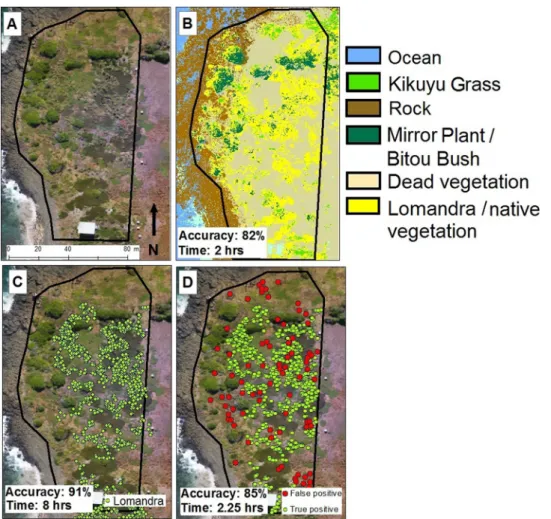
Fig. 10.A. raw UAV image mosaic for the selected weed management and planting area (May 2018), B. Pixel based classiﬁed image, C. Manually digitisedLomandra, D. CNN machine learning results.

Fig. 11.Average producer’s accuracy for mappingLomandraplants, estimated via bootstrapping for each of the mapping approaches evaluated (twentyﬁve cal-culations, 74 ground referencing points). Vertical bars indicate standard error.

(16)

reliably be discerned across the full areal extent of Big Island (Kikuyu Grass, Coastal Morning Glory, Mirror Bush, native vegetation and dead vegetation). The two maps that identified individual Lomandra tus-socks, generated either through manual digitisation or automated de-tection (approaches 2 and 3, respectively) emerged as the most accu-rate, however, they took longer to produce. The three different mapping approaches generated fundamentally different digital information in the form of either a geographically continuous grid depicting a suite of

ﬁve diﬀerent vegetation community components (approach 1) or lo-calised point datasets identifying the location of individualLomandra

tussocks (approaches 2 and 3). The fundamentally diﬀerent nature of the vegetation maps invites greater consideration of the management objectives for which the mapping exercise is being undertaken.

The CNN machine learning algorithm established in the production of the third map emerged as a promising technique for detecting Lomandra plants as it leveraged information from both the high spatial resolution and the spatial context of the raster grids of the UAV images, while also explicitly incorporating spatial relationships within the ar-chitecture of the learning framework.

Declaration of Competing Interest

The authors declare that they have no known competingﬁnancial interests or personal relationships that could have appeared to inﬂ u-ence the work reported in this paper.

Acknowledgements/ Funding

We are indebted to the Berrim Nuru Environmental Services of the Illawarra Local Aboriginal Land Council, staﬀof NSW National Parks and Wildlife Service and the Friends of Five Islands volunteers for their hard work on the vegetation regeneration program, particularly hand planting manyLomandra longifoliaplants throughout the course of the project. UAV surveys were conducted under the National Parks and Wildlife Service Scientiﬁc Licence SL101878 with funding from the GeoQuest Research Institute (University of Wollongong). The vegeta-tion rehabilitavegeta-tion project has been funded by Foundavegeta-tion for Navegeta-tional Parks and Wildlife, NSW Environmental Trust Grant and the Port Kembla Community Investment Fund.

CRediT authorship contribution statement

S.M. Hamylton:Conceptualization, Data curation, Formal analysis, Funding acquisition, Investigation, Methodology, Project administra-tion, Resources, Software, Supervision, Validaadministra-tion, Visualizaadministra-tion, Writing - original draft, Writing - review & editing. R.H. Morris:

Conceptualization, Data curation, Funding acquisition, Project admin-istration, Writing - review & editing.R.C. Carvalho:Conceptualization, Data curation, Formal analysis, Writing - review & editing.N. Roder:

Data curation, Formal analysis, Investigation, Validation, Writing -original draft.P. Barlow:Data curation, Formal analysis, Investigation, Validation, Writing - original draft. K. Mills:Supervision, Writing -review & editing. L. Wang: Methodology, Software, Supervision, Writing - review & editing.

Appendix A. Supplementary data

Supplementary material related to this article can be found, in the online version, at doi:https://doi.org/10.1016/j.jag.2020.102085.

References

Agisoft, L.L.C., 2014. Agisoft PhotoScan User Manual, professional edition..

Barlow, P., 2018. A comparative study of raster and vector based approaches in vegeta-tion mapping on Five Islands oﬀthe coast of Port kembla. School of Earth and Environmental Sciences (p. 132). University of Wollongong.

Blaschke, T., Lang, S., Hay, G., 2008. Object-based Image Analysis: Spatial Concepts for Knowledge-driven Remote Sensing Applications. Springer Science & Business Media.

Bottou, L., Vapnik, V., 1992. Local learning algorithms. Neural Comput. 4, 888–900.

Carlile, N., Lloyd, C., Morris, R., Battam, H., Smith, L., 2017. Seabird islands: big Island, Five Islands Group, New South Wales. Corella 41, 57–62.

Chenari, A., Erfanifard, Y., Dehghani, M., Pourghasemi, H., 2017. Woodland mapping at single-tree levels using object-oriented classiﬁcation of unmanned aerial vehicle (UAV) images. Int. Arch. Photogramm. Remote Sens. Spatial Inf. Sci. 42.

Colefax, A.P., Butcher, P.A., Kelaher, B.P., Browman, H.E.H., 2017. The potential for unmanned aerial vehicles (UAVs) to conduct marine fauna surveys in place of manned aircraft. Ices J. Mar. Sci. 75, 1–8.

Congalton, R.G., Green, K., 2008. Assessing the Accuracy of Remotely Sensed Data: Principles and Practices. CRC press.

Davis, L.M., 1983. Notes on the Terrestrial Ecology of the Five Islands. Zoology Department, Sydney University.

Domingos, P., 2015. The Master Algorithm: How the Quest for the Ultimate Learning Machine Will Remake Our World. Basic Books.

Dujon, A.M., Schoﬁeld, G., 2019. Importance of machine learning for enhancing ecolo-gical studies using information-rich imagery. Endanger. Species Res. 39, 91–104.

Gao, J., Liao, W., Nuyttens, D., Lootens, P., Vangeyte, J., Pižurica, A., He, Y., Pieters, J.G., 2018. Fusion of pixel and object-based features for weed mapping using unmanned aerial vehicle imagery. Int. J. Appl. Earth Obs. Geoinf. 67, 43–53.

Ghazal, M., Al Khalil, Y., Hajjdiab, H., 2015. UAV-based remote sensing for vegetation cover estimation using NDVI imagery and level sets method. 2015 IEEE International Symposium on Signal Processing and Information Technology (ISSPIT) 332–337 IEEE.

Gonzalez, L., Montes, G., Puig, E., Johnson, S., Mengersen, K., Gaston, K., 2016. Unmanned aerial vehicles (UAVs) and artiﬁcial intelligence revolutionizing wildlife monitoring and conservation. Sensors 16, 97.

Hamylton, S., 2017. Spatial Analysis of Coastal Environments. Cambridge University Press.

Husson, E., Ecke, F., Reese, H., 2016. Comparison of manual mapping and automated object-based image analysis of non-submerged aquatic vegetation from very-high-resolution UAS images. Remote Sens. (Basel) 8, 724.

Krishna, K.R., 2016. Push Button Agriculture: Robotics, Drones, Satellite-guided Soil and Crop Management. Apple Academic Press.

Lawley, V., Lewis, M., Clarke, K., Ostendorf, B., 2016. Site-based and remote sensing methods for monitoring indicators of vegetation condition: an Australian review. Ecol. Indic. 60, 1273–1283.

LeCun, Y., Boser, B.E., Denker, J.S., Henderson, D., Howard, R.E., Hubbard, W.E., Jackel, L.D., 1990. Handwritten digit recognition with a back-propagation network. Advances in Neural Information Processing Systems (pp. 396-404).

LeCun, Y., Bottou, L., Bengio, Y., Haﬀner, P., 1998. Gradient-based learning applied to document recognition. Proc. Ieee 86, 2278–2324.

LeCun, Y., Bengio, Y., Hinton, G., 2015. Deep learning. Nature 521, 436.

Lefsky, M.A., Cohen, W.B., Parker, G.G., Harding, D.J., 2002. Lidar remote sensing for ecosystem studies: lidar, an emerging remote sensing technology that directly mea-sures the three-dimensional distribution of plant canopies, can accurately estimate vegetation structural attributes and should be of particular interest to forest, land-scape, and global ecologists. BioScience 52, 19–30.

Mather, P.M., Koch, M., 2011. Computer Processing of Remotely-sensed Images: an Introduction. John Wiley & Sons.

Matsugu, M., Mori, K., Mitari, Y., Kaneda, Y., 2003. Subject independent facial expression recognition with robust face detection using a convolutional neural network. Neural Netw. 16, 555–559.

Mills, K., 1990. Terrestrial vegetation of big Island, the Five Islands Group, port Kembla, New South Wales: 1938-1989. An historical and ecological study. Illawarra Vegetation Studies 3. Coachwood Publishing, Jamberoo, NSW June.

Mills, K., 2015. Vegetation of the Oceanic Islands of the NSW South Coast 9. Big Island, The Five Islands Group, Illawarra Coast: Exploration, exploitation and conservation. Illawarra Vegetation Studies 46. Coachwood Publishing, Jamberoo, NSW March.

Organ, M.K., Speechley, C., 1997. Illawarra Aborigines-An Introductory History.

Sandino, J., Gonzalez, F., Mengersen, K., Gaston, K.J., 2018. UAVs and machine learning revolutionising invasive grass and vegetation surveys in remote arid lands. Sensors 18, 605.

Viljanen, N., Honkavaara, E., Näsi, R., Hakala, T., Niemeläinen, O., Kaivosoja, J., 2018. A novel machine learning method for estimating biomass of grass swards using a photogrammetric canopy height model, images and vegetation indices captured by a drone. Agriculture 8, 70.

Xie, Y., Sha, Z., Yu, M., 2008. Remote sensing imagery in vegetation mapping: a review. J. Plant Ecol. 1, 9–23.

Zhu, X.X., Tuia, D., Mou, L., Xia, G.-S., Zhang, L., Xu, F., Fraundorfer, F., 2017. Deep learning in remote sensing: a comprehensive review and list of resources. Ieee Geosci. Remote. Sens. Mag. 5, 8–36.