On the Pricing and Hedging of Long Dated Zero Coupon Bonds

Full text

(1)�� . QUANTITATIVE FINANCE RESEARCH CENTRE. QUANTITATIVE FINANCE RESEARCH CENTRE Research Paper 185. September 2006. On the Pricing and Hedging of Long Dated Zero Coupon Bonds Eckhard Platen. ISSN 1441-8010. www.qfrc.uts.edu.au.

(2) On the Pricing and Hedging of Long Dated Zero Coupon Bonds. Eckhard Platen. 1. September 19, 2006. Abstract. The pricing and hedging of long dated derivative contracts is a challenging area of research. As a result of utility indifference pricing for general payoffs the growth optimal portfolio turns out to be the appropriate numeraire or benchmark with the real world probability measure as corresponding pricing measure. This concept of real world pricing can be applied for valuing long dated derivatives. An equivalent risk neutral probability measure does not need to exist under this benchmark approach. This paper develops a parsimonious model for a stock index dynamics, which is based on a time transformed squared Bessel process. It uses a diversified world stock index as proxy for the growth optimal portfolio. Surprisingly low prices result for long dated zero coupon bonds that can be replicated using historical data. Such prices and hedges are difficult to explain under the prevailing risk neutral approach.. 1991 Mathematics Subject Classification: primary 62P05; secondary 60G35, 62P20. JEL Classification: G10, G13 Key words and phrases: growth optimal portfolio, benchmark approach, real world pricing, expected utility maximization, utility indifference pricing, long dated zero coupon bonds, minimal market model.. 1. University of Technology Sydney, School of Finance & Economics and Department of Mathematical Sciences, PO Box 123, Broadway, NSW, 2007, Australia.

(3) 1. Introduction. The growth optimal portfolio (GOP) was discovered in Kelly (1956) and is the portfolio that maximizes expected logarithmic utility from terminal wealth. It appears in a stream of literature including, for instance, Long (1990), Karatzas & Shreve (1998), Becherer (2001), Platen (2002, 2004), Goll & Kallsen (2003) and Karatzas & Kardaras (2006). Collectively, this literature demonstrates that the GOP plays a unifying role in derivative pricing and portfolio optimization. Under the prevailing arbitrage pricing theory, see for instance Ross (1976), Harrison & Kreps (1979), Long (1990), Constatinides (1992), Delbaen & Schachermayer (1994), Rogers (1997), Cochrane (2001) and Duffie (2001), several authors refer for the pricing of assets under the real world probability to the closely related numeraire portfolio, state price density, pricing kernel, deflator or stochastic discount factor. In a risk neutral setting the numeraire portfolio equals the GOP, see Bajeux-Besnainou & Portait (1997), Becherer (2001), Platen (2004) and Karatzas & Kardaras (2006). By using the GOP as numeraire and the real world probability as pricing measure, the real world pricing concept, see, for instance, Platen (2002) and Platen & Heath (2006), does not require the existence of an equivalent risk neutral probability measure. The paper establishes via utility indifference pricing, see Davis (1997), the real world pricing concept for nonreplicable payoffs. To apply real world pricing effectively, in practice, it is of great importance that the GOP can be directly observed and its dynamics realistically modeled. This paper will argue that the world stock portfolio can be used as a proxy for the GOP. When discounted, it will be modeled by a time transformed squared Bessel process. By assuming a deterministic time transformation this yields a parsimonious model, the minimal market model (MMM), see Platen (2001, 2002), for the world stock index with the long term net growth rate of the discounted GOP as the main parameter. This model does not admit an equivalent risk neutral probability measure. The resulting surprisingly low prices for long dated zero coupon bonds and their demonstrated hedge are difficult to explain under the standard risk neutral approach. This paper demonstrates that the richer class of models that becomes available under the benchmark approach is essential for realistic modeling of the long term dynamics of the market. The paper is structured as follows. Section 2 introduces a financial market model. Section 3 discusses utility maximization, utility indifference pricing and the market portfolio in relation to the GOP. Section 4 derives the minimal market model and hedges long dated zero coupon bonds.. 2.

(4) 2. Financial Market Model. The modeling of the financial market is based on a filtered probability space (Ω, A, A, P ), with filtration A = (At )t∈[0,∞) , satisfying the usual conditions, see Karatzas & Shreve (1991). We consider a market where trading activity is modeled by the market time τ = {τt , t ∈ [0, T ]}, T ∈ [0, ∞), which is a potentially random nondecreasing adapted process. The market time τt is assumed to be such that τT < ∞ almost surely. A random market time allows subordination in the sense of Clark (1973). The trading uncertainty is modeled by standard Wiener processes W k = {Wτk , τ ∈ [0, ∞)}, k ∈ {1, 2, . . . , d}, which evolve in market time. Since market time is permitted to jump randomly one can model event driven trading uncertainties that could generate significant dependencies of jumps in asset prices. It allows also the modeling of Lévy process driven asset price dynamics as suggested, for instance, in Carr et al. (2003). A wide class of random market time processes can be used, however, we do not specify here any further the market time. The financial market comprises d + 1 primary security accounts, d ∈ {1, 2, . . .}, that securitize all investable wealth over the finite time horizon [0, T ]. These include a savings account,n which isolocally riskless and whose value at market time Rt τt is given by Sτ0t = exp 0 rs ds for t ∈ [0, T ], where rt denotes the adapted, almost surely finite short rate at time t. They also include d nonnegative, savings account discounted, risky primary security accounts S̄ j = {S̄τj , τ ∈ [0, τT ]}, j ∈ {1, 2, . . . , d}. Each of these evolves in market time and contains only units of one type of security, typically shares of stocks, with all proceeds reinvested. To specify the dynamics of the jth discounted risky primary security account we assume that its value S̄τj , j ∈ {1, 2, . . . , d}, satisfies the stochastic differential equation (SDE) Ã ! d X k dS̄τj = S̄τj pjτ dτ + bj,k (1) τ dWτ k=1. S0j. bj,k τ. for τ ∈ [0, τT ] with > 0. Here denotes the volatility of the jth primary security account with respect to the kth Wiener process W k and pjτ the corresponding risk premium. The risk premia and volatilities are assumed to form adapted left continuous processes in market time, satisfying the integrability conditions Z τT X Z τT X d X d d ¡ j,k ¢2 bτ dτ < ∞ and |pjτ | dτ < ∞ 0. 0. j=1 k=1. j=1. almost surely. Note that in the given incomplete market the market time, risk premia, short rate and volatilities can be influenced by uncertainties that are not modeled by the Wiener processes W 1 , W 2 , . . . , W d . We call a predictable stochastic process δ = {δ τ = (δτ0 , δτ1 , . . . , δτd )> , τ ∈ [0, τT ]} a strategy if for all j ∈ {0, 1, . . . , d} and τ ∈ [0, τT ] the Itô stochastic integral 3.

(5) Rτ. δsj dS̄sj exists. Here δτj , j ∈ {0, 1, . . . , d}, denotes the number of units of the jth primary security account at market time τ ∈ [0, τT ] in the discounted Pd held δ δ j j portfolio S̄τ . Then S̄τ = j=0 δτ S̄τ is the value of the corresponding discounted portfolio at the market time τ . A strategy δ and the corresponding S̄ δ are said to be self-financing if d X δ dS̄τ = δτj dS̄τj (2) 0. j=0. for τ ∈ [0, τT ]. In what follows we consider only self-financing strategies and portfolios and will, therefore, omit the phrase “self-financing”. d To avoid obvious arbitrage we assume that the volatility matrix bτ = [bj,k τ ]j,k=1 j,k d ]j,k=1 for all τ ∈ [0, τT ]. We now is invertible with inverse matrix b−1 = [b−1 τ τ k introduce the market price of risk θτ at the market time τ with respect to W k , k ∈ {1, 2, . . . , d}, as a component of the vector ¡ ¢> θ τ = θτ1 , θτ2 , . . . , θτd = b−1 (3) τ pτ. for τ ∈ [0, τT ], with pτ = (p1τ , p2τ , . . . , pτd )> denoting the vector of risk premia. It will be convenient to characterize a nonzero portfolio in terms of the fractions of its wealth invested in the primary security accounts. The jth fraction is given at market time τ by S̄ j j (4) πδ,τ = δτj τδ S̄τ for j ∈ {0, 1, . . . , d} and τ ∈ [0, τT ]. P Some of these fractions may be negative, but j they always sum to one such that dj=0 πδ,τ = 1 for all τ ∈ [0, τT ]. In terms of fractions a strictly positive, discounted portfolio satisfies then the SDE dS̄τδ. =. S̄τδ. d X d X. ¡ k ¢ j πδ,τ bj,k θτ dτ + dWτk τ. (5). k=1 j=1. for τ ∈ [0, τT ]. We will demonstrate that a key to the understanding of the long term market dynamics will be obtained from the study of the growth optimal portfolio (GOP), which was introduced by Kelly (1956). One can demonstrate in various mathematical manifestations that the GOP outperforms all other strictly positive portfolios. For instance, in the long run its path outperforms almost surely that of any other strictly positive portfolio, see Platen (2004). Consequently, it represents a natural benchmark for investment management. To identify a GOP let S̄ δ be a strictly positive discounted portfolio. By the Itô formula we obtain for its logarithm the SDE d ln(S̄τδ ). =. gτδ. dτ +. d X d X k=1 j=1. 4. j k πδ,τ bj,k τ dWτ ,. (6).

(6) where the growth rate gτδ at market time τ is given by  !2  Ã d d d X X X 1 j j k   gτδ = πδ,τ bj,k πδ,τ bj,k τ θτ − τ 2 j=1 j=1 k=1. (7). for τ ∈ [0, τT ]. A strictly positive, discounted portfolio S̄ δ∗ is called a discounted GOP if for all strictly positive, discounted portfolios S̄ δ the inequality gτδ∗ ≥ gτδ holds almost surely, for all τ ∈ [0, τT ]. The first order conditions with the maximization of (7) yield the optiP associated j,k for all τ ∈ [0, τT ] and j ∈ {1, 2, . . . , d}. Thus, mal fractions πδj∗ ,τ = dk=1 θτk b−1 τ by (5) the SDE for a discounted GOP in market time is dS̄τδ∗ = S̄τδ∗. d X. ¢ ¡ θτk θτk dτ + dWτk. (8). k=1. for τ ∈ [0, τT ]. We fix the strictly positive initial value S̄0δ∗ > 0 and call S̄ δ∗ the discounted GOP. Now, we refer to any security expressed in units of the GOP as benchmarked. By the Itô formula the benchmarked value Ŝτδ =. S̄τδ S̄τδ∗. (9). of the portfolio with strategy δ satisfies the SDE dŜτδ. =. d X j=0. δτj. Ŝτj. d X ¡. ¢ k k bj,k τ − θτ dWτ. (10). k=1. for τ ∈ [0, τT ]. Since there is no drift term in (10), Ŝ δ is a local martingale and one can prove the following fundamental property, see Platen (2002): Lemma 2.1 tingale.. Any benchmarked nonnegative portfolio is an (A, P )-supermar-. This supermartingale property allows to preclude the following weak form of arbitrage which resonates the real life constraint of limited liability: For any nonnegative benchmarked portfolio Ŝ δ with zero capital its supermartingale ³ initial ¯ ´ δ ¯ δ property yields the relation 0 = Ŝ0 ≥ E ŜτT A0 ≥ 0, and, therefore, the equality P (ŜτδT > 0) = 0. In other words, nonnegative portfolios are absorbed at zero whenever they reach zero. In economic language this can be interpreted as the absence of a weak form of arbitrage, see Loewenstein & Willard (2000) and Platen (2002). Note that the only ingredient for excluding such weak arbitrage 5.

(7) is the existence of the GOP, which itself is a consequence of the invertibility of the volatility matrix. We emphasize that an equivalent risk neutral probability measure does not need to exist in the given framework. We call a portfolio or price process fair if when benchmarked forms an (A, P )martingale. The fair price process UH = {UH (τ ), τ ∈ [0, τT ]} of a replicable nonnegative payoff H with delivery at maturity T satisfies then at time t ∈ [0, T ] the real world pricing formula ¶ µ H ¯¯ δ∗ (11) UH (τt ) = Sτt E ¯ At < ∞. SτδT∗ Here the GOP Sτδ∗ = S̄τδ∗ Sτ0 is used as numeraire, see Long (1990) and Platen (2002), and the real world probability as pricing measure. From an economic point of view the fair portfolio that replicates a given replicable payoff provides the correct price for this claim since its benchmarked value is a martingale and, thus, by Lemma 2.1 the minimal replicating nonnegative portfolio. It is straightforward to show that when an equivalent risk neutral probability measure exists, the real world pricing formula (11) coincides with the standard risk neutral pricing formula, see Platen (2002).. 3. Utility Indifference Pricing. In the given incomplete market it is important to have a rationale for the consistent pricing of nonreplicable payoffs. For this purpose we will employ utility indifference pricing and, therefore, consider expected utility maximization. We consider a twice differentiable, strictly increasing and strictly concave utility function U : [0, ∞) → <, whose derivative U 0 is invertible with inverse U 0−1 , and where U 0 (0) = ∞ and U 0 (∞) = 0. Let us maximize for the time horizon T ∈ (0, ∞) the finite expected utility from discounted terminal wealth ³ ¡ ¢¯ ´ ¯ v δ̃ = max+ E U S̄τδT ¯ A0 < ∞. (12) S̄ δ ∈V̄x. Here the maximum is taken over the set V̄x+ of all discounted, strictly positive, fair portfolios S̄ δ with initial capital S̄0δ = x > 0. We emphasize that the minimal nonnegative hedge portfolio for a nonnegative replicable payoff is the corresponding fair portfolio and it makes not much sense to consider other portfolios than fair portfolios. We prove in Appendix A the following result. Theorem 3.1 If the benchmarked savings account Ŝ 0 = {Ŝτ0 = is a scalar diffusion process in market time, and ¯ ´ ³ ´ ³ ¯ û(τt , Ŝτ0t ) = E U 0−1 λ Ŝτ0T Ŝτ0T ¯ At < ∞ 6. 1 , S̄τδ∗. τ ∈ [0, τT ]} (13).

(8) for all t ∈ [0, T ], with λ such that x =. û(0,Ŝ00 ) , Ŝ00. then the discounted portfolio. S̄τδ̃t = S̄τδt∗ û(τt , Ŝτ0t ) maximizes the above expected utility from discounted terminal wealth. This portfolio has the fraction 1 Ŝτ0 ∂ û(τ, Ŝτ0 ) =1− Jτδ̃ û(τ, Ŝτ0 ) ∂ Ŝ 0. (14). invested at market time τ ∈ [0, τT ] in the GOP and holds the remainder of its wealth in the savings account. Under the alternative stock index model that we will derive below, Ŝ 0 is a scalar diffusion process in market time, as requested by the above theorem. This theorem can be interpreted as a two-fund separation theorem in the spirit of Tobin (1958). The quantity Jτδ̃ in (14) plays the role of a risk aversion coefficient in the sense of Pratt (1964). Under the assumptions of Theorem 3.1 let us consider a market participant who uses the utility function U with time horizon T ∈ (0, ∞). Let us consider a nonnegative, potentially nonreplicable payoff H that is AT -measurable with E( SHδ∗ ) < ∞, delivered at time T . We now determine for the payoff H and an T expected utility maximizing market participant a price that is consistent with her or his utility function U . To solve this problem we apply utility indifference pricing in the sense of Davis (1997). This will yield the price at which the market participant is indifferent between entering the derivative contract or investing according to the expected utility maximizing strategy δ̃. Consider now a contract which delivers the nonnegative payoff H at time T with candidate price V at time t = 0. Let the market participant buy a very small positive fraction ε > 0 of the contract at time t = 0 for the amount εV and invest x − εV units of her or his wealth according to the expected utility maximizing strategy δ̃ obtained in Theorem 3.1. Similarly as in (12) we then introduce the expected utility function Ã Ã !¯ ! δ̃ ¯ (x − ε V ) S̄ τT δ̃ (15) vε,V =E U + εH̄ ¯¯ A0 x with discounted payoff H̄ = SH0 . We call the value V in (15) the utility indifferτT ence price of the payoff H if δ̃ δ̃ vε,V − v0,V =0 ε→0 ε. lim. (16). almost surely. Based on this definition we derive in Appendix B the following result:. 7.

(9) Theorem 3.2 Under the assumptions of Theorem 3.1 the utility indifference price UH (0) at time t = 0 of a nonnegative, potentially nonreplicable, nonnegative payoff H that is delivered at time T , satisfies the real world pricing formula (11) provided that for¯ all AT -measurable κ ∈ (0, 1) and all Ṽ in a neighborhood of the value S0δ∗ E( SHδ∗ ¯ A0 ) < ∞ the expectation τT ¯  Ã ¯ ! !Ã ¯ ¯ µ µ ¶Ã ¶!2 ¯ ¯ ¯ ¯ λ Ṽ λ Ṽ 00 0−1 0−1 ¯ E U U ¯ A0 ¯ ≤ K + κ H̄ H̄ − U 1 − κ ¯ ¯ ¯ x x S̄τδt∗ S̄τδT∗ ¯ ¯ (17) is uniformly bounded by some constant K < ∞. This theorem makes the important statement that the utility indifference price of a nonreplicable payoff does not depend on the utility function and forms a fair price process. The technical condition (17) is not restrictive. It is satisfied for a wide range of utility functions and payoffs under the stock index model that we will derive below.. 4. An Stock Index Model. Above we have shown that the GOP plays a crucial role as benchmark in investment management and as numeraire in derivative pricing. Therefore, it is of major interest to identify this portfolio in the market and to model its dynamics. In Platen (2005) a diversification theorem is derived which is, in principle, model independent and only requires some regularity property of the market. It states that any portfolio, where all fractions get smaller with increasing number d of primary securities, is a proxy for the GOP. Consequently, if one assumes that the market portfolio (MP) of investable stocks is such a diversified portfolio, then one deals with a proxy of the GOP. Furthermore, it has been shown in Platen (2006), that Sharpe ratio maximization leads to two fund separation into the GOP and the savings account. Such type of two fund separation is also obtained under expected utility maximization in Theorem 3.1. Now, let us discuss the situation when each market participant has her or his investable wealth at all times invested with some fraction in the GOP and the remainder in the savings account. The discounted value S̄τδMP of the MP satisfies in this case an SDE of the type ¢−1 ¡ |θτ | (|θτ | dτ + dWτ ), (18) dS̄τδMP = S̄τδMP JτδMP qP d k 2 for τ ∈ [0, τT ], with total market price of risk |θτ | = k=1 |θτ | and the stochasP tic differential dWτ = |θ1τ | dk=1 θτk dWτk of the Wiener process W , see Platen & 8.

(10) Heath (2006). Obviously, if the MP has all wealth invested in the GOP, then the MP equals the GOP, which corresponds to an ideal risk aversion coefficient of JτδMP = 1. This situation is consistent with the above mentioned diversification theorem, where the fractions in all primary security accounts, including the savings account, are becoming smaller with increasing number of stocks in the market. For simplicity, we assume from now on a constant risk aversion coefficient JτδMP = J δMP > 12 . We plot in Figure 1 the logarithm of a reconstructed discounted MP for the 7 ln(discounted MP) ln(average). 6. 5. 4. 3. 2. 1 1926. 1950. 1975. 2000. Figure 1: Logarithm of the discounted market portfolio. world stock market for the period from January 1926 until March 2006, based on monthly data, provided by Global Financial Data. This discounted MP is denominated in units of the US dollar savings account and can be interpreted as a world stock index. For simplicity, we set in the remainder the market time equal to calendar time, that is τt = t for t ∈ [0, T ]. One notes in Figure 1 that the logarithm of the discounted MP fluctuates around a linearly regressed line, which increases with some net growth rate η with respect to calendar time. In Figure 1 we estimate η = 0.052. In the following we aim to capture the dynamics of S̄ δMP in a parsimonious stock index model. On the basis of the identified average long term exponential growth in Figure 1 we parameterize the SDE (18) of the discounted MP by its drift in terms of the simple exponential drift function ¢−1 ¡ |θt |2 = α exp {η τ } (19) αtδMP = S̄tδMP J δMP t ∈ [0, T ], with an initial scale parameter α > 0. This parametrization of the SDE (18) is a departure from the usual parametrization in asset price modeling where the volatility s |θt | = J δMP. αtδMP S̄tδMP J δMP. 9. (20).

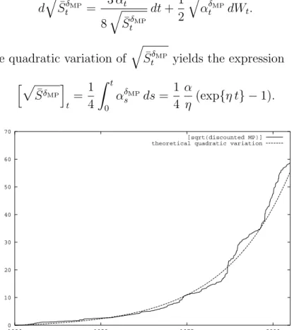
(11) is typically taken as key parameter process. By substituting (19) and (20) into the SDE (18) we obtain s S̄tδMP αtδMP dS̄tδMP = αtδMP dt + dWt (21) J δMP for all t ∈ [0, T ]. It is evident from (21) that the discounted MP is a time transformed squared Bessel process of dimension 4J δMP , see Revuz & Yor (1999). This observation is practically very useful, since much is known about the distributional properties of squared Bessel processes. To simplify our analysis even further we choose the ideal risk aversion J δMP = 1. For q identifying the initial scale parameter α from historical data let us analyze S̄tδ∗ . By the Itô formula one obtains the SDE q q 3 αtδMP 1 δMP dt + αtδMP dWt . d S̄t = q 2 8 S̄tδMP q Therefore, the quadratic variation of hp. i S̄ δMP. t. 1 = 4. Z. t 0. S̄tδMP yields the expression. αsδMP ds =. 1α (exp{η t} − 1). 4 η. 70 [sqrt(discounted MP)] theoretical quadratic variation 60. 50. 40. 30. 20. 10. 0 1926. 1950. 1975. 2000. √. Figure 2: Observed quadratic variation [ S̄ δMP ]t and its theoretical value. We plot in Figure 2 the observed quadratic variation and its theoretical value when setting α = 0.183 and η = 0.052, which provides a good fit. We refer to the above model as the minimal market model (MMM), see Platen (2001). The key parameters of this parsimonious model are the net growth rate η > 0 and the initial scale parameter α > 0 if we consider the short rate as given. 10.

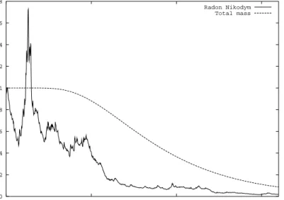
(12) The structure of this stock index model captures several stylized empirical features of stock market indices. For instance, with its negatively correlated volatility (20) it explains the well-documented leverage effect, see Black (1976), but also the observed Student t distributed log-returns of the MP with degrees of freedom four, see Fergusson & Platen (2006). Thus, we obtained a model for a stock market index with two easily estimated parameters. Recall that Ŝt0 denotes the benchmarked savings account. When interpreting S δMP as the GOP in a complete market, the Radon-Nikodym derivative for the Ŝ 0 candidate risk neutral measure equals Λt = Ŝt0 for t ∈ [0, T ]. We show Λt in 0 Figure 3, assuming that the discounted MP equals the discounted GOP. The 1.8 Radon Nikodym Total mass 1.6. 1.4. 1.2. 1. 0.8. 0.6. 0.4. 0.2. 0 1926. 1950. 1975. 2000. Figure 3: Radon-Nikodym derivative and total mass of the candidate risk neutral measure. observed systematic average decline is due to the long term outperformance of the savings account by the world stock index, see also Dimson, Marsh & Staunton (2002). Since under the stylized MMM Λ = {Λt , t ∈ [0, T ]} is the inverse of a time transformed squared Bessel process of dimension four, it follows from Revuz & Yor (1999) that Λ is an (A, P )-strict supermartingale. This is consistent with the observation of a systematically declining trajectory in Figure 3. The candidate risk neutral measure is under the MMM not equivalent to the real world probability measure P . Using the above estimated parameters we show in Figure 3 also the total mass ½ ¾ ¡ ¯ ¢ 2 η S̄0δ∗ ¯ (22) E Λt A0 = 1 − exp − α (exp{η t} − 1) of the candidate risk neutral measure as a function of time t ∈ [0, T ]. The explicit expression in (22) is obtained by integrating against the analytically available transition density of the squared Bessel process of dimension four, see Platen (2002). 11.

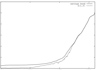
(13) It can be demonstrated that the MMM implies the existence of “free lunches with vanishing risk”, in the sense of Delbaen & Schachermayer (1994, 1998). The situation is not desperate, however, since the MMM does not allow the weak form of arbitrage discussed earlier, see Platen (2002). A non-replicable payoff can be consistently priced via the real world pricing formula (11) when using Theorem 3.2.. Pricing and Hedging of Long Dated Zero Coupon Bonds The pricing and hedging of long dated derivative contracts has been a challenging problem in finance and insurance. Since we derived a model for the dynamics of the MP we can now study its applicability for pricing and hedging long dated contracts on such a stock index. In the case of a nonnegative payoff H with maturity date T we obtain its price according to Theorem 3.2 by the real world pricing formula (11). If H is independent of the value STδ∗ of the GOP at maturity T , then the actuarial pricing formula µ ¶ ¡ ¯ ¢ H ¯¯ δ∗ PH (t, T ) = St E A = P1 (t, T ) E H ¯ At (23) δ∗ ¯ t ST follows directly from (11) for t ∈ [0, T ]. Here P1 (t, T ) denotes the zero coupon bond price at time t with payoff H = 1 at maturity T . We emphasize that the actuarial pricing formula (23) is of central importance in insurance. Its key ingredients are the expectation of the independent payoff H under the real world probability and the zero coupon bond price. Now, using (22) we obtain under the above stylized MMM with deterministic short rate for the zero coupon bond price the explicit formula ½ Z T ¾µ ½ ¾¶ 2 η S̄τδt∗ P1 (t, T ) = exp − rs ds 1 − exp − (24) α (exp{η T } − exp{η t}) t for t ∈ [0, T ]. For illustration, let us interpret the historically observed US short rate as being deterministic. This allows us to plot in Figure 4 the evolution of the price of the zero coupon bond at time t which matures at T in March 2006 using the stylized MMM with the above estimated n parameters. o In the same RT ∗ figure we display also the savings bond P (t, T ) = exp − t rs ds as a function of t ∈ [0, T ]. The zero coupon bond has an initial value of P1 (0, T ) = 0.0042 which represents only about 8.5% of the initial savings bond value P ∗ (0, T ) = 0.0495. The key property of the benchmarked zero coupon bond is that it is a martingale, whereas the benchmarked savings bond is a strict supermartingale. Since both replicate the same payoff at time T , the martingale determines the lowest price for the payoff H = 1, which forms a fair price process. Note that under the benchmark approach different self-financing portfolios can replicate the same payoff. Only for fair portfolios one has the law of one price. 12.

(14) 1.2 savings bond P(t,T). 1. 0.8. 0.6. 0.4. 0.2. 0 1926. 1950. 1975. 2000. Figure 4: Zero coupon bond and savings bond. Theoretically, the payoff H = 1 can be replicated at time T by investing at time t ∈ [0, T ] δ∗ (t) =. ∂P1 (t, T ) ∂Stδ∗ ∗. = P (t, T ) exp. ½. −2 η S̄tδ∗ α (exp{η T } − exp{η t}). ¾. 2η (25) α (exp{η T } − exp{η t}). units in the MP and the remainder in the savings account with continuous reallocation of the wealth. For illustration we perform a hedge simulation, where we calculate the selffinancing portfolio that starts at the theoretical initial zero coupon bond price P1 (0, T ) and keep during each following month the number of units invested as determined by (25). It turns out that the hedge portfolio almost perfectly replicates with monthly rehedging the payoff of the zero coupon bond at maturity T . We plot in Figure 5 the resulting benchmarked profit and loss of the hedge portfolio, which remains very close to zero. The resulting zero coupon bond has an initial value, which is far less than that of the savings bond. This phenomenon is difficult to explain under the risk neutral approach even if one considers stochastic interest rates. However, under the benchmark approach it can be easily explained as a consequence of the strict supermartingale property of the benchmarked savings account. These findings raise serious concerns about the use of risk neutral pricing and hedging for long dated derivative contracts in finance and insurance. Forthcoming work will demonstrate for long dated index and currency derivatives similar explanatory power of the above stylized MMM.. 13.

(15) 8e-006. 6e-006. 4e-006. 2e-006. 0. -2e-006. -4e-006. -6e-006. -8e-006 1926. 1950. 1975. 2000. Figure 5: Benchmarked profit and loss.. Acknowledgement The author likes to express his thanks to Hardy Hulley, Ioannis Karatzas, Truc Le, Harry Markowitz, Martin Schweizer and Xun Yu Zhou for their valuable comments and stimulating interest in this work. Furthermore, support by the ARC grant DP 0559879 is acknowledged.. Appendix A: Proof of Theorem 3.1 We express the constrained optimization problem (12), which maximizes over discounted, fair portfolios, by introducing a Lagrange multiplier λ ∈ (0, ∞) in the functional µ µ δ ¯ ¶ ¶ ³ ¡ ¢¯ ´ ³ ¡ ¢¯ ´ S̄τT ¯ x ¯ ¯ δ δ v = E U S̄τT ¯ A0 − λ E (26) A = E F S̄τδT ¯ A0 − ¯ 0 δ∗ S̄τδT∗ S̄0 that has to be maximized for S̄ δ ∈ V̄x+ . When maximizing the function F (S̄τδT ) = ³ S̄ δ ´ U (S̄τδT ) − λ S̄τδT∗ − S̄xδ∗ with respect to S̄τδT one obtains the first order condiτT. tion U 0 (S̄τδT ) −. λ ∗ S̄τδT. 0. = 0. Since U is concave, U 0 (0) = ∞ and U 0 (∞) = 0, this. characterizes a maximum. By applying the inverse function U 0−1 of U 0 on both sides of the ³first ´ order condition it follows for the candidate optimal portfolio that λ δ̃ 0−1 S̄τT = U . Since S δ̃ is assumed to be a fair portfolio one needs to choose S̄ δ∗ τT. λ ∈ (0, ∞) such that S̄0δ̃ x = =E S̄0δ∗ S̄0δ∗. Ã. S̄τδ̃T ¯¯ ¯ A0 S̄τδT∗. !. µ =E U. 14. µ 0−1. λ S̄τδT∗. ¶. ¶ 1 ¯¯ ¯ A0 . S̄τδT∗. (27).

(16) Since Ŝτ0 = (S̄τδ∗ )−1 is a scalar diffusion process in market time τ there exists by the Feynman-Kac formula a function û(·, ·) such that µ µ ¶ ¶ ¯ ´ ³ ³ ´ λ 1 ¯¯ 0 0−1 0 ¯ δ̃ 0−1 0 Ŝτt = û(τt , Ŝτt ) = E U A = E U λ Ŝ Ŝ (28) ¯ t τT τT ¯ At S̄τδT∗ S̄τδT∗ forms an (A, P )-martingale for t ∈ [0, T ]. It is straightforward to verify that the resulting strategy δ̃, with the fraction (14) invested in the GOP, maximizes the expected utility. ¤. Appendix B: Proof of Theorem 3.2 The following expected utility difference can be derived from (15) by the Taylor expansion in the form ¯ Ã ¯ Ã !¯ ! ¯ 1¯ ¯ δ̃ ³ ´ ³ ´ ¯ S̄ 1 ¯¯ δ̃ ¯ τ δ̃ ¯ δ̃ ¯ ε ¯vε,V − v0,V ¯ ≤ ¯E U S̄τδ̃T + U 0 S̄τδ̃T ε H̄ − V T ¯¯ A0 − v0,V ¯+ K, ¯ 2 ε ε¯ x (29) ³ ´ λ δ̃ 0−1 , which yields due to (29) and (17) see (17). We have from (13) S̄τT = U S̄ δ∗ τT. for the utility indifference price V the relation Ã ´ 1 ³ δ̃ λ δ̃ 0 = lim vε,V − v0,V =E ε→0 ε S̄τδT∗ µ µ ¶ H ¯¯ V ³ δ̃ = λ E ¯ A0 − E ŜτT Sτδt∗ x. Ã. S̄τδ̃ H̄ − V T x ¶ ¯ ´ ¯ A0 .. !¯ ! ¯ ¯ A0 ¯ (30). This provides for the payoff H the real world formula (11) when exploiting ³ pricing ¯ ´ δ̃ δ̃ ¯ ¤ the martingale property of Ŝ , where E ŜτT A0 = Ŝ0δ̃ = S̄xδ∗ . 0. References Bajeux-Besnainou, I. & R. Portait (1997). The numeraire portfolio: A new perspective on financial theory. The European Journal of Finance 3, 291– 309. Becherer, D. (2001). The numeraire portfolio for unbounded semimartingales. Finance Stoch. 5, 327–341. Black, F. (1976). Studies in stock price volatility changes. In Proceedings of the 1976 Business Meeting of the Business and Economic Statistics Section, American Statistical Association, pp. 177–181. Carr, P., H. Geman, D. Madan, & M. Yor (2003). Stochastic volatility for Lévy processes. Math. Finance 13(3), 345–382. 15.

(17) Clark, P. K. (1973). A subordinated stochastic process model with finite variance for speculative prices. Econometrica 41, 135–159. Cochrane, J. H. (2001). Asset Pricing. Princeton University Press. Constatinides, G. M. (1992). A theory of the nominal structure of interest rates. Rev. Financial Studies 5, 531–552. Davis, M. H. A. (1997). Option pricing in incomplete markets. In M. A. H. Dempster and S. R. Pliska (Eds.), Mathematics of Derivative Securities, pp. 227–254. Cambridge University Press. Delbaen, F. & W. Schachermayer (1994). A general version of the fundamental theorem of asset pricing. Math. Ann. 300, 463–520. Delbaen, F. & W. Schachermayer (1998). The fundamental theorem of asset pricing for unbounded stochastic processes. Math. Ann. 312, 215–250. Dimson, E., P. Marsh, & M. Staunton (2002). Triumph of the Optimists: 101 Years of Global Investment Returns. Princeton University Press. Duffie, D. (2001). Dynamic Asset Pricing Theory (3rd ed.). Princeton, University Press. Fergusson, K. & E. Platen (2006). On the distributional characterization of log-returns of a world stock index. Appl. Math. Finance 13(1), 19–38. Goll, T. & J. Kallsen (2003). A complete explicit solution to the log-optimal portfolio problem. Ann. Appl. Probab. 13(2), 774–799. Harrison, J. M. & D. M. Kreps (1979). Martingale and arbitrage in multiperiod securities markets. J. Economic Theory 20, 381–408. Karatzas, I. & C. Kardaras (2006). The numeraire portfolio and arbitrage in semimartingale models of financial markets. Statistics Department, Columbia University (working paper). Karatzas, I. & S. E. Shreve (1991). Brownian Motion and Stochastic Calculus (2nd ed.). Springer. Karatzas, I. & S. E. Shreve (1998). Methods of Mathematical Finance, Volume 39 of Appl. Math. Springer. Kelly, J. R. (1956). A new interpretation of information rate. Bell Syst. Techn. J. 35, 917–926. Loewenstein, M. & G. A. Willard (2000). Local martingales, arbitrage, and viability: Free snacks and cheap thrills. Econometric Theory 16(1), 135– 161. Long, J. B. (1990). The numeraire portfolio. J. Financial Economics 26, 29–69. Platen, E. (2001). A minimal financial market model. In Trends in Mathematics, pp. 293–301. Birkhäuser. Platen, E. (2002). Arbitrage in continuous complete markets. Adv. in Appl. Probab. 34(3), 540–558. 16.

(18) Platen, E. (2004). A benchmark framework for risk management. In Stochastic Processes and Applications to Mathematical Finance, pp. 305–335. Proceedings of the Ritsumeikan Intern. Symposium: World Scientific. Platen, E. (2005). Diversified portfolios with jumps in a benchmark framework. Asia-Pacific Financial Markets 11(1), 1–22. Platen, E. (2006). A benchmark approach to finance. Math. Finance 16(1), 131–151. Platen, E. & D. Heath (2006). A Benchmark Approach to Quantitative Finance. Springer Finance. Springer. Forthcoming. Pratt, J. W. (1964). Risk aversion in the small and in the large. Econometrica 32, 122–136. Revuz, D. & M. Yor (1999). Continuous Martingales and Brownian Motion (3rd ed.). Springer. Rogers, L. C. G. (1997). The potential approach to the term structure of interest rates and their exchange rates. Math. Finance 7, 157–176. Ross, S. A. (1976). The arbitrage theory of capital asset pricing. J. Economic Theory 13, 341–360. Tobin, J. (1958). Estimation of relationships for limited dependent variables. Econometrica 26, 24–36.. 17.

(19)

No results found