Exploiting Group Sparsity in SAR Tomography
Xiao Xiang Zhu
(1,2), Nan Ge
(1), Muhammad Shahzad
(2)(1) Remote Sensing Technology Institute (IMF) German Aerospace Center (DLR) Oberpfaffenhofen, 82234 Wessling, Germany Email: {xiao.zhu, nan.ge, muhammad.shahzad}@dlr.de
(2) Helmholtz Young Investigators Group “SiPEO” Chair of Remote Sensing Technology
Technische Universität München Arcisstraße 21, 80333 Munich, Germany Abstract—With meter-resolution images delivered by modern
SAR satellites like TerraSAR-X and TanDEM-X, it is now possible to map urban areas from space in very high level of details using advanced interferometric techniques such as persistent scatterer interferometry and tomographic SAR (TomoSAR), whereas these multi-pass interferometric techniques are based on a great number of images. We aim at improving the estimation accuracy of TomoSAR while reducing the required number of images by incorporating prior knowledge of buildings into estimation. In this manuscript, we propose a novel workflow that marries the freely available 2D building footprint GIS data and the group sparsity concept for TomoSAR inversion. Experiments on bistatic SAR data stacks demonstrate great potential of the proposed approach, e.g., highly accurate tomographic reconstruction is achieved using six interferograms only.
Keywords— group sparsity; SAR tomography; GIS; TanDEM-X; compressive sensing
I. INTRODUCTION
Modern spaceborne synthetic aperture radar (SAR) sensors, such as TerraSAR-X (TSX), TanDEM-X (TDX) and COSMO-SkyMED, deliver SAR data with very high spatial resolution of up to 1 m. With these meter-resolution data, advanced multi-pass interferometric techniques like persistent scatterer interferometry (PSI) and tomographic SAR (TomoSAR) allow retrieving not only the 3D geometrical shape but also the undergoing temporal motion in the millimeter scale of individual buildings [1]–[5]. In particular, sparse reconstruction based methods [6][7], e.g. SL1MMER [8], give robust TomoSAR inversion with very high elevation resolution, and can offer so far ultimate 3D, 4D and 5D SAR imaging [9][10].
In spite of that, the downside of PSI and TomoSAR is their high data demand. For instance, in the interesting parameter range of spaceborne SAR and by using even the most efficient algorithms, such as non-linear least squares and SL1MMER, 11 is the critical number of acquisitions required to achieve a reasonable reconstruction [8]. “Reasonable” in this context means that given an average signal-to-noise ratio (SNR) of 6 dB, the detection rate of double scatterers with a distance of one Rayleigh resolution unit reaches 90%. However, if we can extract certain detailed features or patterns of high-rise buildings in SAR images beforehand, the required number of images can be significantly reduced by incorporating such features as prior for a joint estimation.
For this purpose, we propose a novel workflow marrying the globally available 2D building footprint GIS data and the group sparsity concept for TomoSAR inversion.
II. PRIOR KNOWLEDGE RETRIEVAL
We work with bistatic high resolution spotlight TSX/TDX interferograms with cross-track baselines ranging between approximately ±200 m. The single-pass characteristic renders path delay effects very small and deformation negligible. For this reason these datasets are ideal to test our proposed methodology.
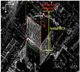
In order to retrieve prior information pertaining to building regions, 2D building footprints are downloaded from OpenStreetMap (OSM). The first necessary step is to perform 2D transformation to project the vertices of these footprints from world coordinates to SAR azimuth-range coordinates. Fig. 1 shows the resulting projected reference polygon as (red and green) solid lines overlaid onto our building of interest.
The procedure continues by identifying the side of the building footprint facing the SAR sensor. If we assume that
1,..., i n
v= denote the indices of ordered 2D footprint vertices of
one particular building. Then any vertex vk
(
k n∈)
belongs to the side facing the sensor if and only if its projection onto the line at zeroth range axis (i.e., line defined as rg = 0 with zero azimuth slope) does not self-intersect the reference polygon. The range of total number of vertices belonging to side visible to the sensor in any footprint is m where 1< ≤m n. The inequality that m > 1 depicts that, if not occluded, at least one side or two vertices of the building are always visible to the side looking SAR sensor.Once the vertices that face the sensor are identified, we compute the region of interest (ROI) polygon, denoted as
ROI
poly , by translating the identified vertices at a distance d
towards the sensor. We initialize d according to the height of the tallest building in this area. To elaborate how the polyROI
is computed, consider a building having four vertices
1 2 3 4 1
v v v v v− − − − where − denotes the adjacency i.e., v2 is adjacently connected to v1 and v3, and so on. Now if the vertices v2, v3 and v4 are visible or facing the sensor, then the
ROI
poly is formed as v v v v v v v1− − − − − −2 2′ 3′ 4′ 4 1, where for j = 2, 3, and 4, v′j
(
rg az,)
=vj(
rg d az− ,)
.Afterwards, we perform morphological operations to compute the number of background pixels (num) in the ROI image I derived using polyROI from the SAR image. If num is
less than a specified threshold TH, then the desired building mask is generated otherwise the procedure is repeated by re-computing polyROI using d d= −5. I.e., the already shifted
vertices (i.e., v v2′ ′, and 3 v4′) are progressively shifted 5m away from the sensor or towards the building footprint (see Fig. 1). In other words, starting with bigger polygonal region, the algorithm recursively reduces the polygon till it finds the best match.
Following the extraction of building mask, pixels sharing similar height are then grouped together in a nearest-neighbor manner.
Fig. 1. Building mask extraction with reference polygon (shown in red and green solid polylines) of our building of interest, overlaid onto the SAR intensity map after geocoding. Side of the building facing the sensor is shown in red while the other side not visible to the sensor in green. Vertices connecting the red polyline are shifted towards the sensor as depicted by dotted yellow lines forming an initial ROI which is recursively reduced to the region shown by red dotted lines.
III. GROUP SPARSITY IN TOMOSAR
In this section, we first revisit a data model commonly used in TomoSAR, as well as the SL1MMER algorithm. Following this, we extend the SL1MMER algorithm to the multiple snapshot case. The extended version exploits group sparsity and is named as M-SL1MMER.
A. TomoSAR System Model
After acquisition, raw SAR data will be focused onto the azimuth-range (x-r) plane. During this process, information along the third dimension, the so-called elevation axis s
perpendicular to x-r, is lost. I.e., echoes from, e.g., ground, building facade and roof sharing the same distance to the sensor, are mapped onto one single pixel. To reconstruct s and to separate those different contributions, TomoSAR utilizes scenes acquired from slightly different viewing angles to synthesize an elevation aperture Δb along s (cf. aperture along
x created by steering radar beam) for full 3D SAR imaging. A
well-established model, which can be found, e.g., in [11], is given by
,
= +
g R γ ε (1)
where g∈N×1 is the single snapshot observation vector with each entry gn sampled irregularly at the elevation frequency
n
ξ , R∈N L× is the sensing matrix with exp( 2 )
nl n l
R = −j pξ s , 1
L×
∈
γ is the unknown reflectivity vector with each element
( )
l slγ =γ assigned to the discrete elevation position sl, and 1
N×
∈
ε is the additive noise vector. Typically we haveNL, which renders (1) underdetermined. Note that motion has been neglected in this context without loss of generality.
Similar to azimuth resolution, the elevation counterpart ρs is inversely proportional to Δb [11]. For the high resolution spotlight TSX/TDX data w.r.t. our test area, ρs is about 24.9 m, being much worse than the corresponding azimuth and range resolution (approx. 1.10 and 0.588 m, respectively) due to tight orbit control.
B. The SL1MMER Algorithm
To tackle (1), an algorithm called SL1MMER, which stands for Scale-down by L1 norm Minimization, Model selection, and Estimation Reconstruction, has been proposed in [8] to achieve both accuracy and robustness. SL1MMER has been originally designed for TomoSAR in urban areas, under the assumption that there are only a few dominant scatterers (phase centers) along s within each x-r pixel [2]. I.e., γ has merely K non-zero entries with typically K = 0, 1, 2, or 3. As its name suggests, this algorithm consists of the following three main steps.
1) Scale-down by L1 Norm Minimization
To exploit the sparse prior on γ, the Least Absolute Shrinkage and Selection Operator (LASSO) method based on the L1 norm of γ is used
2 2 1 1 ˆ arg min , 2 λK = − + γ γ g Rγ γ (2)
where λK is a hyperparameter balancing model error and the sparsity of γ. LASSO is known to deliver robust elevation estimates of dominant scatterers. Therefore, by identifying the most significant entries in γˆ and choosing corresponding columns of R, the dimension of the original problem can be downscaled by a large factor. However, LASSO is prone to amplitude bias as a result of L1 norm relaxation and introduces
outliers when certain mathematical conditions of R are not fully satisfied (as is the case for most real-world problems). In this regard, the next two steps are deemed necessary.
2) Model Selection
The initial estimate γˆ from (2) may contain artifacts, which falsifies its sparsity level K. In order to get rid of them, the model’s goodness of fit should be penalized by its
complexity to avoid overfitting of data. Model selection can be regarded as the following optimization problem
( )
(
)
( )
{
ˆ}
ˆ argmin ln , C , K K= − p g θ K K + K (3) where p(
g θˆ( )
K K,)
is the likelihood function of g given the estimate of unknown θ(K) and K, C(·) is the penalty term for model complexity. By choosing an appropriate penalty criterion, (3) can be solved to estimate the most likely positionsˆ
s of non-zero elements in γˆ, which further shrinks R. This leaves only one last step to correct amplitude bias.
3) Parameter Estimation
At this stage, we have a much slimmer sensing matrix
which we define as ˆ ˆ
( )∈ N K×
R s and thereby (1) transforms into
( ) ( )
ˆ ,ˆ= +
g R s γ s e (4) where γ s( )ˆ ∈Kˆ 1×, and e∈N×1 is the aggregate of both measurement noise and the error introduced by model selection. Since (4) is probably overdetermined, it can be solved with L2 norm minimization
( )
(
H( ) ( )
)
1 H( )
ˆ ˆ = ˆ ˆ − ˆ ,γ s R s R s R s g (5) where (·)H denotes Hermitian transpose.
The Cramér–Rao lower bound (CRLB) for elevation estimate ˆs has been derived for single- and double-scatterer case in [12] and [8], respectively.
C. The M-SL1MMER Algorithm
We extend the SL1MMER method to M-SL1MMER, i.e., for the multiple snapshot case. By applying the method described in section II, we already have M pixels along an iso-height line. We assume that within each of these pixels, there is a dominant scatterer located on building façade. Hence, those
M scatterers should reside at the same height or elevation position. For each pixel, we have, similar to (1),
, m = m m+ m
g R γ ε (6)
{
1, ,}
m M
∀ = . If the iso-height line stretches principally in azimuth direction, we expect ξn to vary little among all concerned pixels. For this reason, we define
1≅ 2 ≅ ≅ m =:
R R R R by using identical discretization of s. Thus, we can rewrite (6) as
,
= +
G R Γ Ε (7)
where G=
[
g1, , gM]
is the observation matrix with Msnapshots, Γ=
[
γ1, , γM]
is the unknown reflectivity matrix with each row corresponding to a discrete elevation position, and E accounts for both additive noise and model error.Eq. (7) is again an underdetermined system with NL. Since we assume that each snapshot has a contribution from the same elevation position of building façade, the non-zero entries of Γ are aligned in a row-wise fashion. Indeed, there can be more non-zero rows related to ground, lower infrastructures, building roof, etc. Still, the number of non-zero rows of Γ is very limited. This property of signals is also referred to as group sparsity. To solve (7) while incorporating this prior, ˆΓ
can be estimated using the group LASSO method [13] 2 F 2,1 1 ˆ argmin , 2 λK = − + Γ Γ G RΓ Γ (8)
where ⋅F denotes the Frobenius norm, and
(
2)
1 2 2,1 1 1 L M lm l= m= γ =∑ ∑
Γ is known to promote group
sparsity. Different polarimetric channels or neighboring pixels were used similarly in [14][15].
After the downscaling step based on the estimate from (8), model selection and parameter estimation will be performed individually for each pixel as the original SL1MMER algorithm suggests.
IV. EXPERIMENTS USING SIMULATED AND REAL DATA
First of all, we evaluate the performance of the proposed M-SL1MMER algorithm using simulated data. We synthesize ground-façade interactions of two scatterers spaced by decreasing elevation distances, which is a well-known benchmark TomoSAR simulation setting [2][6]. Four scenarios are taken into account with N = 11, 6 and SNR = 10, 3 dB due to the following reasons:
- As mentioned in section I, 11 is the critical number of interferograms for a reasonable reconstruction if SL1MMER is used [8]; in the case of two scatterers, 6 is the number of unknowns, namely the amplitude, phase and elevation positon of each scatterer;
- SNR of 3 and 10 dB are usually considered as a lower and an upper bound for persistent scatterers, respectively [16]. For each elevation distance, we independently generate 100 simulations with each containing 48 snapshots, i.e. M = 48, which is an average case for the test building in Fig. 1. λK is
chosen adaptively such that each non-zero element or row position stays consistent while tuning it within a certain range.
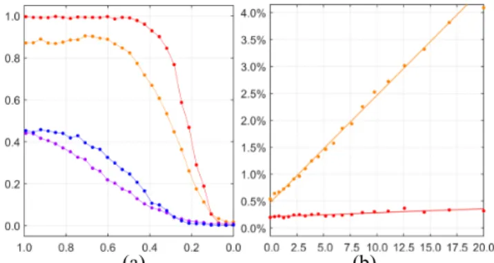
We solve the LASSO and group LASSO problems separately, and follow strictly the rest of SL1MMER procedures to perform model selection and parameter estimation. In Fig. 2a, the detection rate PD is shown for N = 11 w.r.t. the true elevation distance of scatterers from façade and ground, normalized to ρs. We define detection for the case in which not only two scatterers are distinguished, but also their estimates should be bounded by ±3×CRLB of their true elevation. Note that CRLB increases with decreasing elevation distance due to the mutual interference of two scatterers [8]. The red and orange lines denote PD for SNR = 10 dB with M-SL1MMER and M-SL1MMER, while lines in blue and violet are plotted for SNR = 3 dB, again with M-SL1MMER and
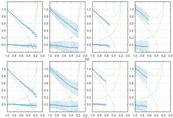
SL1MMER, respectively. Moreover, false alarm rate PF is illustrated in Fig. 2b as a function of SNR for M-SL1MMER (red) and SL1MMER (orange), respectively. For the case N = 6, the gain of using multiple snapshots regarding PD and PF is comparable. Elevation estimates are shown in Fig. 3, where each dot depicts sample mean of all estimates, with error bar indicating the corresponding standard deviation. The true elevation profiles would be two line segments, one on off-diagonal related to building façade and the other parallel to the x-axis related to ground. Green dashed lines mark true elevation profiles ±1×CRLB. Missing points suggest that detection rate is below 25%. Overall, the elevation estimation accuracy of SL1MMER approaches CRLB and degrades with decreasing elevation distance. On the other hand, M-SL1MMER offers not only much smaller estimation variance, but also better super-resolution (cf. Fig. 2a). SL1MMER performs in particular much more inferiorly with small N and low SNR. On the contrary, even for the case N = 6, reasonable profiles are reconstructed with M-SL1MMER.
In addition, M-SL1MMER is applied to the bistatic TSX/TDX data mentioned in section II. The results are compared to those obtained using SL1MMER. Fig. 4 shows the reconstructed and color-coded elevation of our test building, overlaid with intensity. From left to right, the originally superimposed and now separated scatterers, namely first layer with SL1MMER and SL1MMER, second layer with M-SL1MMER and M-SL1MMER, are represented respectively.
On the top of our test building, reflections from building roof and façade are overlaid. In Fig. 4, dominating scattering from roof (red) can be seen in the first layer, whereas the corresponding parts of façade are visible in the second layer. Besides, parallelogram patterns in the second layer can be attributed to reflections within window frames. We do not expect many reflections from lower structures though, due to the large slope of the shell-like roof in front of the test building. It is evident that M-SL1MMER significantly outperforms SL1MMER. In particular, when N = 6, i.e., using extremely small number of scenes, the second layer estimated using SL1MMER is deteriorated by false alarms (cf. Fig. 2b) while M-SL1MMER still achieves reasonable results.
(a) (b)
Fig. 2. Detection rate PD and false larm rate PF with N = 11, and (a) PD w.r.t.
true elevation distance between façade and ground; (b) PF w.r.t. SNR in [dB].
Red and orange lines denote M-SL1MMER and SL1MMER, respectively, so do the lines in blue and violet. In (a), red and orange lines are plotted for the case SNR = 10 dB, while blue and violet lines are for SNR = 3 dB.
V.
C
ONCLUDINGR
EMARKSIn this paper, a novel framework is proposed which can improve the estimation accuracy of TomoSAR while reducing the required number of images. The core idea is the exploitation of group sparsity within iso-height SAR pixel clusters that can be identified with the support of online available GIS data – 2D building footprints. Experiments on simulated and real bistatic TSX/TDX data stacks demonstrate the great potential of the proposed approach. In the future, we will extend the proposed M-SL1MMER for higher dimensional spectral estimation problems, e.g. differential tomographic SAR reconstruction.
ACKNOWLEDGMENT
This work is supported by the Helmholtz Association under the framework of the Young Investigators Group “SiPEO” (VH-NG-1018, www.sipeo.bgu.tum.de) and International Graduate School of Science and Engineering, Technische Universität München (Project 6.08: “4D City”).
REFERENCES
[1] S. Gernhardt, N. Adam, M. Eineder, and R. Bamler, “Potential of Very High Resolution SAR for Persistent Scatterer Interferometry in Urban Areas,” Ann. GIS, vol. 16, no. 2010–06, pp. 103–111, 2010. [2] X. X. Zhu and R. Bamler, “Very High Resolution Spaceborne SAR
Tomography in Urban Environment,” IEEE Trans. Geosci. Remote Sens., vol. 48, no. 12, pp. 4296–4308, 2010.
[3] D. Reale, G. Fornaro, A. Pauciullo, X. Zhu, and R. Bamler, “Tomographic Imaging and Monitoring of Buildings With Very High Resolution SAR Data,” Geosci. Remote Sens. Lett. IEEE, vol. 8, no. 4, pp. 661–665, Jul. 2011.
[4] X. X. Zhu and M. Shahzad, “Facade Reconstruction Using Multiview Spaceborne TomoSAR Point Clouds,” IEEE Trans. Geosci. Remote Sens., vol. 52, no. 6, pp. 3541–3552, Jun. 2014.
[5] G. Fornaro, F. Lombardini, A. Pauciullo, D. Reale, and F. Viviani, “Tomographic Processing of Interferometric SAR Data: Developments, applications, and future research perspectives,” IEEE Signal Process. Mag., vol. 31, no. 4, pp. 41–50, Jul. 2014.
[6] X. Zhu and R. Bamler, “Tomographic SAR Inversion by L1-Norm Regularization -- The Compressive Sensing Approach,” IEEE Trans. Geosci. Remote Sens., vol. 48, no. 10, pp. 3839–3846, 2010.
[7] A. Budillon, A. Evangelista, and G. Schirinzi, “Three-Dimensional SAR Focusing From Multipass Signals Using Compressive Sampling,” Geosci. Remote Sens. IEEE Trans. On, vol. 49, no. 1, pp. 488 –499, Jan. 2011.
[8] X. X. Zhu and R. Bamler, “Super-Resolution Power and Robustness of Compressive Sensing for Spectral Estimation With Application to Spaceborne Tomographic SAR,” IEEE Trans. Geosci. Remote Sens., vol. 50, no. 1, pp. 247–258, 2012.
[9] X. Zhu and R. Bamler, “Demonstration of Super-Resolution for Tomographic SAR Imaging in Urban Environment,” IEEE Trans. Geosci. Remote Sens., vol. 50, no. 8, pp. 3150–3157, 2012.
[10] X. X. Zhu and R. Bamler, “Superresolving SAR Tomography for Multidimensional Imaging of Urban Areas: Compressive sensing-based TomoSAR inversion,” Signal Process. Mag. IEEE, vol. 31, no. 4, pp. 51–58, Jul. 2014.
[11] G. Fornaro, F. Serafino, and F. Soldovieri, “Three-dimensional focusing with multipass SAR data,” IEEE Trans. Geosci. Remote Sens., vol. 41, no. 3, pp. 507–517, Mar. 2003.
[12] R. Bamler, M. Eineder, N. Adam, X. Zhu, and S. Gernhardt, “Interferometric Potential of High Resolution Spaceborne SAR,”
Photogramm. - Fernerkund. - Geoinformation, vol. 2009, no. 5, pp. 407–419, Nov. 2009.
[13] D. Malioutov, M. Cetin, and A. S. Willsky, “A sparse signal reconstruction perspective for source localization with sensor arrays,”
IEEE Trans. Signal Process., vol. 53, no. 8, pp. 3010–3022, Aug. 2005.
[14] E. Aguilera, M. Nannini, and A. Reigber, “Multisignal Compressed Sensing for Polarimetric SAR Tomography,” IEEE Geosci. Remote Sens. Lett., vol. 9, no. 5, pp. 871–875, Sep. 2012.
[15] M. Schmitt and U. Stilla, “Compressive Sensing Based Layover Separation in Airborne Single-Pass Multi-Baseline InSAR Data,”
IEEE Geosci. Remote Sens. Lett., vol. 10, no. 2, pp. 313–317, Mar. 2013.
[16] N. Adam, R. Bamler, M. Eineder, and B. Kampes, “Parametric estimation and model selection based on amplitude-only data in PS-interferometry,” in ESA FRINGE Workshop, 2005.
(a)
(b)
Fig. 3. Reconstructed elevation of simulated façade and ground with M = 48, (a) N = 11, and (b) N = 6, respectively. Y-axis denotes estimated elevation and x-axis the true elevation distance. Each dot has the sample mean of all estimates as its y value and the corresponding standard deviation as vertical bar. Green dashed lines depict true elevation ±1×CRLB. In each row, from left to right: SNR = 10 dB with M-SL1MMER and SL1MMER, SNR = 3 dB with M-SL1MMER and SL1MMER, respectively.
(a)
(b)
Fig. 4. Reconstructed and color-coded elevation of the test building in two layers, overlaid with intensity, (a) N = 11, and (b) N = 6, respectively. In each row, from left to right: first layer with M-SL1MMER and SL1MMER, second layer with M-SL1MMER and SL1MMER, respectively.