Transport Mode Detection and Classification from Smartphone Sensor Data Using Convolutional Neural Networks

(1)

Sensor Data Using Convolutional

Neural Networks

Adam Bako

School of Science

Thesis submitted for examination for the degree of Master of Science in Technology.

Espoo 29.07.2020

Supervisor

Prof. Alexander Ilin

Advisor

(2)

(3)

Author Adam Bako

Title Transport Mode Detection and Classification from Smartphone Sensor Data Using Convolutional Neural Networks

Degree programme EIT Digital Master School

Major Data Science Code of major SCI3095

Supervisor Prof. Alexander Ilin

Advisor Julien Mineraud

Date 29.07.2020 Number of pages 63 Language English

Abstract

Transportation is a significant component of human lives and understanding how individuals travel is an essential task in many fields. Understanding the modes of transport individuals use can lead to improvements in urban planning, traffic control, human health, and environmental sciences. The goal of transport mode detection and classification is to use smartphone devices as human behavioural sensors, to detect and classify individuals movement continuously. Smartphone devices are suitable for transport mode detection, as they are proliferated in modern societies and contain sensors that are suitable for transport mode detection. These sensors include GPS, accelerometers, gyroscopes, magnetometers, barometers, or microphones. The research in this thesis will focus on transport mode detection and classification using data from motions sensors; accelerometers, gyroscopes, magnetometers, and barometers as they do not contain the sensitive private data that is collected when using GPS or microphones.

Currently, there are two approaches in state of the art in transport mode detection. In the first approach, time and frequency domain features are extracted from the signals of the motion sensors and used as input to decision tree or neural network machine learning models. In the second approach, Convolutional Neural Networks extract features by finding spatial relations in the signal data and using these for classification. This thesis investigates the use of Convolutional Neural Networks, as they have shown to outperform models trained using time and frequency domain features extracted from the data in the state of the art research.

(4)

This research studies the effect of different model architectures on the accuracy of Convolutional Neural Network models when using multiple different sensors as input, as well as focusing on which combinations of sensors produce optimal results. Furthermore, the focus will be evaluating the models on real-world data in order to evaluate the feasibility of deploying applications utilizing transport mode detection. This research compares an optimized model architecture along with preprocessing techniques to state of the art Convolutional Neural Network architectures on real-world data. The best baseline algorithm achieved an overall F1 score of 0.57, while the final optimized achieved an overall F1 score of 0.72 on the testing dataset. The optimal combination of motion sensors is with the accelerometer, gyroscope, and barometer.

Keywords Transport mode detection, Convolutional Neural Network, Smartphone, Motion Sensors, Accelerometer, Gyroscope, Magnetometer, Barometer

(5)

Acknoledgements

In this part of the thesis, I would like to give thanks to all people that provided me with support during the research and writing of my thesis. Firstly, I would like to thank my supervisor professor Alexander Ilin for his tips and expertise in the area of Neural Networks. I would like to thank the advisors from the company, MOPRIM, where I performed my research, Julien Mineraud and Esko Nuutila. They provided a lot of insight into the domain of transport mode detection as well as providing motivation during the process of research. I would also like to thank Luca Scotton for his feedback and advice in the implementation of certain aspects of my code as well as Ignacio Rodriguez Burgos for his feedback and tools provided during the writing of this thesis.

Otaniemi, 29.07.2020

(6)

Symbols and abbreviations

Abbreviations

TMD Transport Mode Detection PCT Personal Carbon Trading FFT Fast Fourier Transform

CNN Convolutional Neural Network DNN Deep Neural Network

NN Neural Network

LSTM Long Short Term Memory RNN Recurrent Neural Network GPS Global Positioning System

A-GPS Assisted Global Positioning System ACC Accelerometer

GYR Gyroscope MAG Magnetometer BAR Barometer

KEH Kinetic Energy Harvester ReLU Rectified Linear Unit EF Early Fusion

MF Middle Fusion LF Late Fusion AF Axis Fusion

(9)

1 Introduction

Transportation is a significant component of the life of humans, whether travelling to work, meeting others or performing other activities. Individuals have a multitude of options in the transport modes they use. All methods of transportation have their positives and negatives; the speed of transport, comfort, cost, and carbon footprint, among others. These characteristics influence the choices of transportation of people across the world. The process of discerning the movement of people is transport mode detection, and it is necessary to understand human movement.

Understanding how and why people move in specific ways is a crucial activity for urban planning, human health, and environmental science. In order to understand the transportation of populations, it has been standard to perform travel studies and creating action plans based on the information gained from these studies. However, large-scale studies are expensive in both the monetary cost and effort and therefore, can only be performed in minimal intervals.

With the widespread adoption of smartphones, there is a possibility to create real-time transport monitoring, that can lead to faster action from the perspectives of urban planning, human health, and the environment. This thesis will focus on research into methods to achieve near-real-time transport mode detection using these smartphone devices.

1.1 Use cases of transport mode detection

The uses of transport mode detection and classification are broad, depending on the problem at hand. This section will illustrate these use-cases to motivate the need for transport mode detection. The main uses of this technology are in transport studies, carbon monitoring and trading, and also fitness and personal mobility tracking.

Transportation studies

Transportation studies are studies performed by cities to discern how people move through them. They help the municipalities make informed decisions on how to improve traffic in the city during the short-term and help make decisions for urban planning in the long term. Classic transportation studies utilize large-scale surveys of citizens, asking about what modes of transport they use and the details surrounding them. However, these surveys only provide static data of a specific period, that might not entail the full detail of people’s movement. These studies are very labour-intensive and challenging to implement correctly and are, therefore, not optimal or

(10)

practical [1][2]. Transportation studies which implement transport mode detection with smartphones have the advantage of being continuous, scalable and contain more detail on the nuances of travel that could be difficult to capture using traditional methods.

Carbon monitoring

Personal transportation is one of the significant contributors to carbon emissions of individuals. Knowing more precisely in which ways a single person or a community uses various modes of transport can help reduce carbon emissions [3]. Individuals can use a smartphone application which monitors transport modes and converts these to values of emissions. Viewing how different modes of transport are less polluting than others can help individuals decide which mode of transport to take. Gamification can be implemented into these applications to motivate users [4], as well as viewing individuals emissions compared to their community.

Carbon Trading

Carbon Trading, or in the case of individual citizens; Personal Carbon Trading (PCT) is still a novel research field. It is the process of allocating citizens with a specific amount of emissions credits and letting people who produce fewer emissions trade these credits with higher emitters. Pilot studies of the impacts of these kinds of policies have been made in various locations, for example in Norfolk Island, Australia [5] or the city of Lahti, Finland. In the city of Lahti, the citizens can opt into the project and receive special credits for emitting less carbon. Citizens use these credits to purchase goods or services in certain stores. The citizens use an application, as shown in Figure 1and Figure 2. This application uses transport mode detection on smartphones to constantly monitor all modes of transport and visualizes this data to the users. The purpose of smartphone applications like this is to visualize how people move, suggest more sustainable modes of transport and transform how people move every day. Transport mode detection enables such application to monitor changes in the behaviour of citizens over long time frames with great detail. However, the accuracy of these systems is still not sufficient to be used on a large scale.

Fitness Tracking

Fitness tracking is a useful technology for the monitoring of personal movement for health. Applications that provide these insights track physical activities such as walking, running, and bicycling. Tracking is either done by having the user start and stop the tracking of the activity, during which the application uses GPS and other

(11)

Figure 1: CitiCap application monitoring transport modes main page.

Figure 2: CitiCap application car-bon trading store.

sensors to gather data about the physical activity, or can be done automatically by applications monitoring when users start and stop physical activity. An excellent example of this automatic approach to fitness tracking would be the Apple Health application. Such applications utilize transport mode detection and classification to find the movement of their users, classify it into specific categories and give further data to the users such as step count or speed.

1.2 Smartphones and sensors

Traditionally transport mode detection has been done by vast surveys and travel studies, which help countries and cities figure out how people in their borders move. In novel approaches, smartphone devices are suitable for transport mode detection, as they are proliferated in modern societies and contain sensors that are suitable for transport mode detection. These sensors include GPS, accelerometers, gyroscopes, magnetometers, barometers, or microphones. The GPS, or Global Positioning

(12)

System, gains information on where a smartphone is at a specific time. Monitoring this movement over time is how many transport mode detection models classify transport modes. Motion sensors such as the accelerometer and gyroscope sense the motion of devices, and barometers, which sense pressure can be used to identify the current elevation of devices, and can be used to measure displacement in elevation. These sensors are becoming very common in smartphone devices nowadays due to their uses in various applications.

The research in this thesis will focus on transport mode detection and classification using data from motions sensors; accelerometers, gyroscopes, magnetometers, and barometers as they do not contain the sensitive private data that is collected when using GPS or microphones.

1.3 Methods for transport mode detection

Transport mode detection using sensors from smartphones has become a topic of research in the past 10 years. The early research in this topic focused on extracting time and frequency domain features from sensor data and training decision tree models to distinguish between various modes of transport. However, in recent years, the research has become more focused on deep learning models with advancements in Convolutional Neural Networks and Long Short Term Memory Networks. Convo-lutional Neural Networks (CNN) are conventional models in image classification that can be used to classify raw signal data, viewing it as a one-dimensional image. The advantages of the CNN is the ability for it to classify signal data instead of features extracted from this data, as feature extraction is a difficult task that requires domain knowledge and can overlook certain essential artefacts in the raw data. However, for CNNs to learn, they require extensive training datasets. Long Short Term Memory Networks are also conventional techniques used in transport mode detection due to their proficiency in remembering long term dependencies in the data. The current state of the art implementations of LSTM networks utilizes convolutional layers for feature extraction, which result in higher accuracies than utilizing handcrafted features.

The research in this thesis investigates the implementation of CNNs using multiple smartphone sensor data as well as the optimal model architecture used for sensor fusion. Improvements in the model architectures of CNNs in transport mode detection with multiple sensors will lead to improvements in the CNN-LSTM architectures in future work.

(13)

1.4 Problem definition

This thesis will focus on how to detect various modes of transport using sensors commonly found in smartphone devices using Convolutional Neural Networks. These sensors being the accelerometer, gyroscope, magnetometer and barometer. The following research questions guide the focus of the research in more detail:

• What is the model architecture that is best suited for a Convolutional Neural Network using multiple sensors as input for transport mode detection?

• Which combination of motion sensors produces the best results in transport mode detection?

• How can raw sensor data be preprocessed to help Convolutional Neural Networks converge optimally and generalize well to real-world data?

The success of the Convolutional Neural Network will be evaluated against state of the art CNN architectures.

1.5 Thesis structure

This thesis contains six different chapters; the Introduction, Background, Real-world data and its characteristics, Materials and Methods, Results, and Discussion.

The Background chapter describes state of the art in transport mode detection. First, it describes all sources of data for transport mode detection and their results. Second, it explains data preprocessing techniques for models utilizing feature extracted data and models utilizing raw signal data are defined. Finally, it explains the different state of the art machine learning models that are used in transport mode detection.

The Real-world data and its characteristics chapter explains the differences between real-world and synthetic lab data. Explaining the challenges of collecting data on various smartphones, by various users, in different conditions and how these can affect the accuracy of transport mode detection. The chapter will also address why the specific state of the art methods are implemented to address these issues.

The Materials and Methods chapter proposes the methods used for collecting the data and explains the characteristics of the data set used for the training of the CNN. It provides explanations for the methods used in recreating state of the art models and their preprocessing techniques. It also proposes the methods used in optimizing the model architecture as well as selecting the optimal set of preprocessing

(14)

techniques on the data, to achieve fast convergence of the model. Finally, the chapter will describe the technologies used to preprocess the data and train the CNN models.

The Results chapter presents the results obtained by implementing the methods of the previous chapter. While the Discussion chapter discusses the results, compares them to the state of the art results and proposes the future work to be done.

(15)

2 Background

This chapter describes state of the art in transport mode detection. First, it describes all sources of data for transport mode detection and their results. Second, it explains data preprocessing techniques for models utilizing feature extracted data and models utilizing raw signal data are defined. Finally, it explains the different state of the art machine learning models that are used in transport mode detection.

2.1 Sources of data

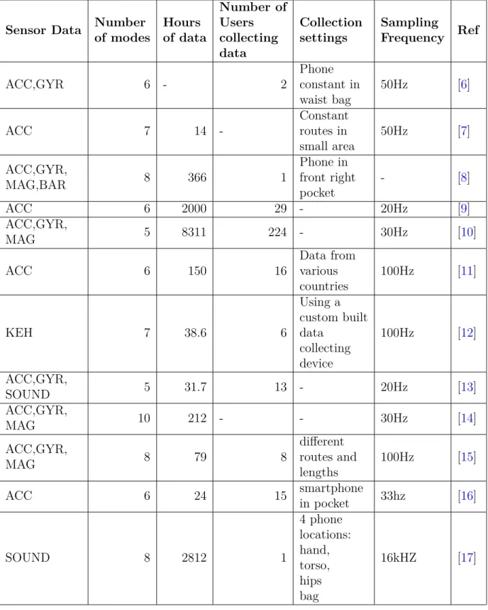
In recent years, research in transport mode detection has shown promising results using a plethora of different data sources. The data sources from different sensors from smartphones all have different advantages and disadvantages. This subsection describes how different sensors are applicable to transport mode detection and what results they have been able to achieve. Furthermore, the datasets, as shown in Table 1, from various research papers are discussed along with the amount of data collected, how data was collected, and the specific sensors they collect.

Global Positioning System

The Global Positioning System (GPS) is a system used to detect the location of devices utilizing satellites in the orbit of the planet [18]. GPS receivers are standard features of smartphones, which receive messages from multiple satellites and use this information to estimate their location. These aggregated GPS points can be used to determine velocities, accelerations, and paths of the device, which lead to the inference of the mode of transport taken by the individual. More concretely, modern smartphones utilize Assisted GPS technology (A-GPS) that enhance the availability of location detection by utilizing cell tower data in combination with satellite data. However, these A-GPS smartphone devices still have a lower location accuracy than dedicated GPS devices [19]. Most smartphone applications can set the required accuracy of the location to a specific radius, as well as the frequency at which this data is collected. Higher frequency and a smaller radius will improve the accuracy but will have a large impact on the battery consumption of the smartphone devices.

Furthermore, the use of GPS data of individuals brings up many privacy concerns, as to track the modes of transport means to track an individuals position constantly. Therefore, there are many drawbacks to the GPS data with specific trade-offs; mainly accuracy, battery consumption, and privacy.

(16)

Sensor Data Number of modes Hours of data Number of Users collecting data Collection settings Sampling Frequency Ref ACC,GYR 6 - 2 Phone constant in waist bag 50Hz [6] ACC 7 14 -Constant routes in small area 50Hz [7] ACC,GYR, MAG,BAR 8 366 1 Phone in front right pocket - [8] ACC 6 2000 29 - 20Hz [9] ACC,GYR, MAG 5 8311 224 - 30Hz [10] ACC 6 150 16 Data from various countries 100Hz [11] KEH 7 38.6 6 Using a custom built data collecting device 100Hz [12] ACC,GYR, SOUND 5 31.7 13 - 20Hz [13] ACC,GYR, MAG 10 212 - - 30Hz [14] ACC,GYR, MAG 8 79 8 different routes and lengths 100Hz [15] ACC 6 24 15 smartphone in pocket 33hz [16] SOUND 8 2812 1 4 phone locations: hand, torso, hips bag 16kHZ [17]

(17)

techniques. Yu et al. [20] used features extracted from GPS trajectories to classify five distinct travel modes using a recurrent neural network to achieve an accuracy of 92.7%.

Jiang et al. [21] use features extracted from GPS trajectories and points passed through a recurrent neural network to classify seven different travel modes with an accuracy of 97.3%

GPS data has also been used to attempt to differentiate between different types of vehicles. In the research of Simoncini et al. [22] features from GPS data are input into a recurrent neural network to classify car types into small-duty, medium-duty, and heavy-duty vehicles, based on their characteristics, namely weight and size. The accuracy of such classifiers was only 56.2%.

Accelerometer

The accelerometer is a sensor that measures the acceleration of the device in 3-dimensional space. It is a typical sensor in modern smartphones due to the appli-cations of the data in mobile gaming, motion input, and orientation sensing [23]. Transport mode detection utilizes the accelerometer by identifying specific patterns of acceleration in the 3-dimensional space and match these patterns to specific modes. The accelerometer sensor also measures the acceleration of gravity. Depending on the orientation of the device, the gravity component will be present on different axes. Gravity is removed from the measurements to create an orientation independent view of the acceleration of the device. The Data preprocessing section of this chapter discusses the removal of gravity in more detail.

The accelerometer can be sampled with various sampling frequencies, which will impact the battery consumption and accuracy of the sensor. The advantage of the accelerometer is that the privacy concerns are not as strong as in the case of GPS, because monitoring the acceleration of the movement of a phone does not give as much private information as tracking their exact location.

The use of the accelerometer in transport mode detection has been studied using various techniques. Immer et al. [24] used features extracted from accelerometer data to classify four different types of transport modes using a recurrent neural network with an accuracy of 92%.

Liang et al. [7] used raw accelerometer data to classify seven different types of transport modes using a convolutional neural network with an accuracy of 94.5 %.

Han et al. [9] used raw accelerometer data with a convolutional neural network to classify different types of human activity, such as moving downstairs, upstairs,

(18)

jogging, walking, sitting and standing, with an accuracy of 98.83%. However, the smartphone device with the accelerometer was set at a fixed position and angle. Most studies specify the strict conditions of data collections, where the accelerometer is set in a fixed position, which does not reflect a real-life use-case, as people use their smartphone devices during modes of transport.

Gyroscope

The Gyroscope is a sensor that measures the angular velocity of the device in three axes and can be used to discern the orientation of the device [23]. They are common in smartphones nowadays due to their uses in mobile gaming. When combined with the accelerometer data, they can provide data about the orientation independent acceleration of the device, and help reduce the noise of the accelerometer data. The Gyroscope itself can only give limited information about transport mode, but when used in conjunction with multiple sensors can give more accurate results [15].

Zhou et al. [6] used features extracted from accelerometer and gyroscope data to classify six different types of transport modes using a recurrent neural network with Long short term memory with an accuracy of 92.8%.

Tambi et al. [25] used spectrogram data from raw accelerometer and gyroscope data to classify four modes of transport with a CNN with 91 %.

Magnetometer

The magnetometer is a sensor that measures the magnetic field strength in three axes. It measures the Earth’s magnetic field using the hall-effect [26]. However, the sensor contains noise from its surroundings. The noise can come from the magnetic fields produced by the components of the smartphones. Noise from magnetic fields also come from devices in the surroundings of the device [27]. As with the Gyroscope, this sensor cannot be used solely for the transport mode detection, but when used in conjunction with multiple sensors, can give more accurate results.

Asci et al. [14] combined the features of an accelerometer, gyroscope and mag-netometer to use as inputs into a recurrent neural network to classify 10 different transport modes with an accuracy of 97.07%.

Guvensan et al. [15] used features extracted from an accelerometer, gyroscope and magnetometer to use as inputs into a random forest classifier; the initial classifi-cation accuracy was 82.3%. However, after post-processing the data using a custom algorithm, the overall accuracy was increased to 95%.

(19)

Barometer

The barometer is a sensor that measures the air pressure surrounding it; this is a single value in hectopascal. This value of pressure can monitor changes in pressure over time; which happen during changes in elevation, changes in pressure due to tunnels, for example in metros, or changes in pressure of a vehicle, for example in aeroplanes [8]. However, barometers are only present in higher-end smartphones as they are not a necessity for the standard uses of cheaper devices. Therefore the implementation of this as a data source can be limiting when addressing the needs of detecting the transport modes of a broad population with different smartphone devices.

Jeyakumar et al. [8] and Qin et al. [28] combined the data from the accelerometer, gyroscope, magnetometer and barometer as inputs for a classifier. They both used a combination of a convolutional neural network and a recurrent neural network and respectively achieved an F1 score of 96.4% and an accuracy of 98.1%.

Sound

The microphone, present in all smartphone devices, is used in transport mode detection by distinguishing specific artefacts in the noise of various modes of transport. The challenge is to isolate the sound of the transport from the environmental noise such as human speech or noise from the location of the device (e.g. friction in pocket). This sensor can distinguish between specific modes of transport, for example, tram and metro, where the acceleration footprints are very similar. However, there are privacy concerns in monitoring the microphone of a smartphone device constantly.

Wang et al. [17] used raw sound data with a convolutional neural network to classify eight different transport modes and achieved an accuracy of 86.6%. When adding the data from extracted features from an accelerometer and gyroscope with the sound data, Carpineti et al. [13] achieved an accuracy of 93% using a random forest classifier.

Bluetooth and WiFi

Location-specific networks such as Bluetooth beacons and public WIFI networks do not hold enough information to classify modes of transport by themselves. However, they can be used to aid in the precision of transport mode detection algorithms. These networks are becoming more widely available in cities—for example, public WiFis in various modes of public transport. Cardoso et al. [16] completed a study in the city of Porto with the use of features extracted from accelerometers and

(20)

the monitoring of public WiFi networks. Cardoso classified five various modes of transport with an accuracy of 95.6%.

Kinetic Energy Harvester

Kinetic Energy Harvesters (KEH) are parts of personal devices that generate electrical energy from vibrations of the device. The output signals of these KEHs, which is the amount of energy they are producing, can be analyzed to classify various modes of transport. The advantages of the KEH as a sensor is in power consumption, which is far lower than an accelerometer. The accelerometer consumes about 85mW while monitoring the KEH signal can consume only 480uW [12]. However, these KEHs are mostly available in smartwatches and fitness, which are not as common as smartphone devices.

Xu et al. [12] used extracted features from the KEH output signal and classified seven different modes of transport with an accuracy of 97%.

2.2 Data Preprocessing

Data preprocessing is an essential step for training machine learning models. There are two main ways approaches to data preprocessing; feature extraction and raw data preprocessing. With feature extraction, the goal is to extract meaningful information from the signal data so that these features can be used to discriminate between various modes. For raw data preprocessing the goal is to prepare the data in a way that models can learn more quickly and generalize better for unknown data and preparing it so the model can easily extract features from the data. This section will explain the process of windowing the data, which is necessary for both feature extraction and raw data preprocessing. After this, feature extraction and raw data preprocessing will be explained in more depth.

Windowing

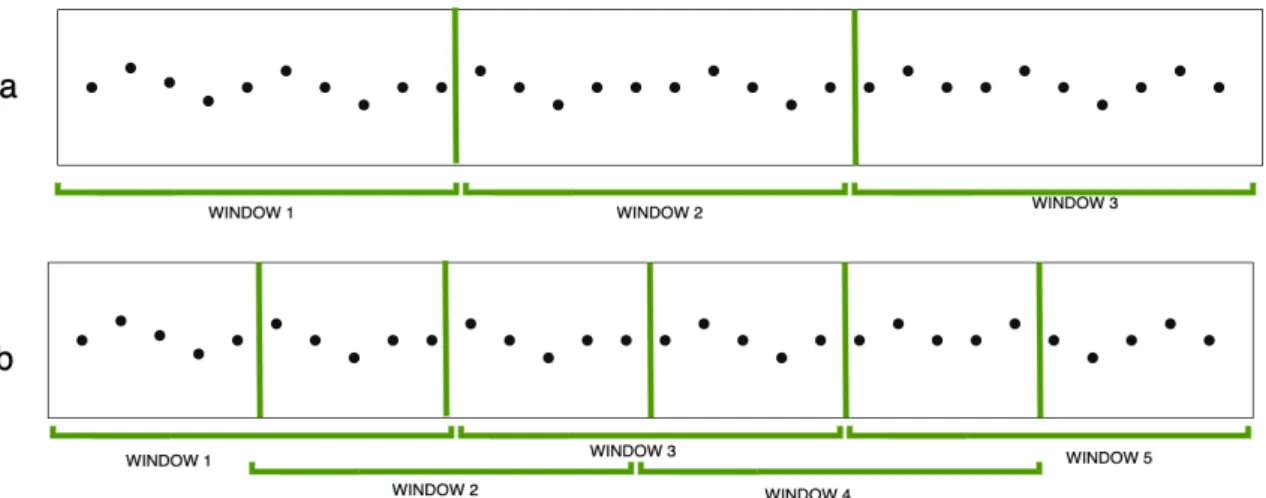
The windowing of the data entails splitting the sensor signal into small fragments, that can be classified individually. Windowing is necessary as windows can be easily compared to each other if they have the same amount of data points. Some models have a fixed input size, where the input data must always be the same number of data points, which requires windowing. Windows are set for an exact number of samples, but can also have an overlap. An overlap in windows means that a certain percentage of the data in one window will be present in the following window, as shown in Figure 3.

(21)

Figure 3: Windowing of data, example a shows windowing with no overlap and b shows windowing with 50% overlap.

The sizes of windows vary due to the different models that use these windows. Bedogni et al. [29] tested various window sizes from 5 seconds to 240 seconds with a Random Forest classifier and found 120-second windows to be most effective. When training a different Random Forest model using a more extensive list of features, Guvesan et al. [15] found 60-second windows with 40% overlap to achieve the best results. However, when training an LSTM model, Guvesan et al. [14] found that 12-second windows performed better than larger 24-second windows. Zhou et al. [30] found that for their Random Forest classifier 20-second windows achieved the highest accuracy. Therefore, window sizes and overlap have to be set and optimized for specific models and extracted features individually.

The most common sizes for windows in raw data preprocessing are 10 seconds. For example, Liang et al [7] and Han et al. [9] use a window size of 10 seconds with no overlap. While some researchers, for example, Tambi et al. [25], use a larger window size of 30 seconds with 50% overlap. The overlap is more necessary for larger windows, as multiple transport modes can be present in such large windows.

Feature Extraction

In order for decision tree models to be able to distinguish between various modes of transport, they must be given specific data to be able to discriminate between the modes. Raw data cannot be used as input due to the complexity of the signal. Features extracted from the raw data better describe the motion that is captured by the sensors. These features include the variance of the data points or the range of the values in the signal. Features can give information on the speed of the transport mode and the acceleration profiles. There are various approaches to the amount of complexity in feature extraction. There are statistical, frequency domain-based,

(22)

Feature Reference

Statistical Mean, Standard Deviation, Minimum Value,

Maximum Value [11],[13],[15],[14] Variance, Median, Range [11],[15],[14] Interquartile Range, Kurtosis, Skewness, RMS [11], [14] Minimum Reduction, Maximum Reduction,

Maximum Increase, Minimum Increase,

Covariance, Harmonic Mean, Quadratic Mean, Arithmetic Mean of Instant Exchange,

Quadratic Mean of Instant Exchange

[15]

Time Integral, Double Integral, Auto-Correlation [11] Mean-Crossing Rate [11], [14] Zero-Crossing Rate [14] Frequency

FFT DC 1,2,3,4,5,6 Hz , Spectral Entropy, Spectrum Peak Position, Wavelet Entropy, Wavelet Magnitude

[11] Spectral Energy [11], [14] Spectral Centroid, Spectral Spread,

Spectral Flatness, Spectral Roll-Off, Spectral Crest, Spectral Kurtosis

[14] Peak Volume, Intensity, Length, Kurtosis, Skewness [11],[28] Segment Variance of Peak Features, Peak Frequency,

Stationary Duration, Stationary Frequency [11],[28]

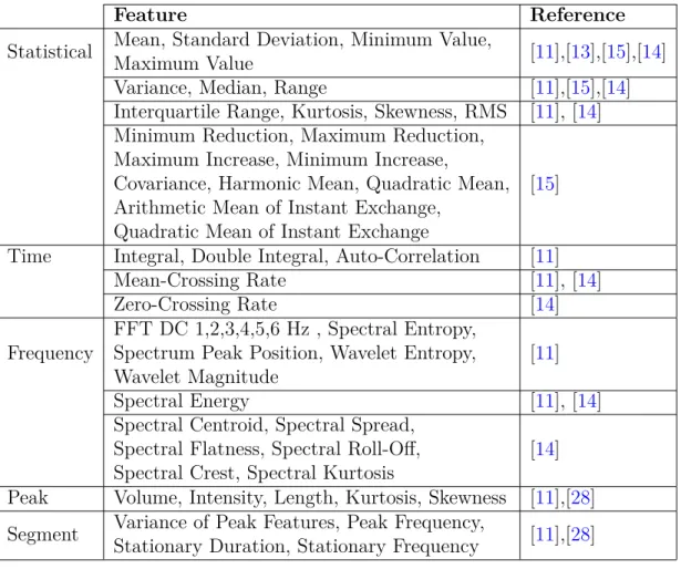
Table 2: Features extracted from motion sensor data from various studies. time-domain based, peak based and segment based features, as shown in Table 2. The table shows the feature type on the leftmost column, the feature names in the middle column and the studies that utilize these specific features in the right column. The statistical features are statistics of the values of the data points. The time-domain features take features from the signal as a whole. The frequency-domain features take information from the frequency domain by using an FFT. The peak and segment based features are based on the research of Hemminki et al. [11], where they extract features when acceleration and deceleration periods are found in the acceleration profile.

Raw Data Preprocessing

Raw sensor data must be preprocessed for it to be used as input for a CNN model. Once the data has been windowed, the data can also be processed to help the weights of the CNN to converge more easily. This processing is done by normalizing the data to a more consistent range. The most common technique for normalization in transport mode detection using motion sensors is Z-Score normalization [9][28][31][32].

(23)

In Z-Score normalization the each data point in a list is normalized using the mean and the standard deviation of that list[33] :

x′_ij = xij −mean(xi) std(xi)

. (1)

In this equation, the i represents the index of the window that is being normalized and j represents the index of a data point in the list of data points in the window being normalized. Some CNN studies utilize MinMax scaling:

x′_ij = xij −min(xi) max(xi)−min(xi)

. (2)

Where the minimum and maximum values are used to normalize the data, to set the range of the data points in the sensor signal between one and zero.

Different approaches to preprocessing the data exist in order for the CNN model to generalize better for the testing data and for the weights and biases to converge stably [28]. The first issue these preprocessing steps are attempting to solve is the effect of gravity on the accelerometer data, as the orientation of the smartphone device will affect which axes are affected by the force of gravity. The removal of the gravity is discussed in the Section2.3. The second issue these preprocessing steps are attempting to solve is the signals in three axes being impacted by the orientation of the device. The horizontal acceleration of the vehicle will be present in different axes of the accelerometer in different orientations of the device. In order to remove this orientation dependence, one possibility is to take the magnitude of the accelerometer:

magacc =

√︂

acc2

x+acc2y +acc2z (3)

Liang et al. [7] argue this removes the issue of varying orientations. The other possibility is to implement a "fusion" layer in the CNN, implemented by Han et al. [9]. This fusion layer is a convolutional layer that takes the three axes of the accelerometer and outputs a single activation map. Han et al. argue that this process also removes the issue of varying orientations.

In a different approach to data preprocessing a spectrogram of the frequencies present in the accelerometer is used as input to the CNN. This method is implemented by Tambi et al. [25]. They argue that this preprocessed data allows the CNN to learn more quickly using a smaller architecture of the model, enabling it to be used on smartphones with limited storage and computing capabilities.

2.3 Gravity estimate and removal

The accelerometer measures the acceleration in three axes. Due to gravity, which is a constant acceleration directing downwards to the earth, the accelerometer

(24)

measurements will be impacted. Depending on the orientation of the device during measurements, the gravitational acceleration will be present on different axes in differing magnitudes. Therefore to decouple the measurements of acceleration caused by transport modes, the impact of gravity on the three axes must be estimated and removed.

There are various filtering methods in order to achieve gravity estimation and removal. Liang et al. [7] propose using a low pass filter to estimate the gravity component and subtract it from the accelerometer values. Hemminki et al. [34] propose a more sophisticated method for removing gravity. Their approach is to detect points in the data where the user is either stationary or moving at a constant velocity, which they call keypoints. In these points, due to the lack of acceleration from other sources, the accelerometer signal contains the gravity component. Once these keypoints are generated, they interpolate the gravity component over time. During this recording of keypoints, they also measure the signal of the gyroscope. When the gyroscope shows a substantial change in orientation, the gravity estimation restarts. The gravity estimate signal in three axes is then removed from the three axes of the accelerometer. In modern smartphones, virtual gravity sensors are present that calculate the gravity using the accelerometer and gyroscope, and record the gravity estimate as a signal in three axes.

2.4 Random Forest models for transport mode detection

Random Forest models are an implementation of the Decision trees that generalize better on data outside of the training data set. Decision trees are models that resemble tree graphs, where features in the data are used to discriminate between specific modes of transport. Random Forest models create an ensemble of decision trees by using subsets of features from the data and during inference gather the results from the ensemble of trees and take the result of the majority as the final classification. In terms of transport mode detection, there have been studies utilizing various features from various sensors with different results, as shown in Table 3. Random Forest models are conventional techniques used to classify transport modes and are often used as baseline algorithms to compare to other models. Random Forest models produce the highest accuracy when compared to other supervised learning algorithms that are not implementations of neural networks, for example, Support Vector Machine classifiers or Naive Bayes classifiers [7].

2.5 Deep Learning models for transport mode detection

In this section, the applications of deep learning models to the task of transport mode detection and classification will be discussed. The two main approaches that

(25)

Model type Sensor data Preprocessing Overall accuracy

Number

of modes Reference Random Forrest ACC, GYR,

SOUND FE 93 5 [13]

Random Forrest ACC,GYR,

MAG FE 92 8 [15]

AdaBoost ACC FE Prec : 64 6 [11]

LSTM ACC,GYR R 93 6 [6] CNN ACC R 94 7 [7] CNN-LSTM ACC,GYR, MAG,BAR R 96 8 [8] CNN ACC R 99 6 [9] DNN ACC,GYR, MAG FE 95 5 [10] LSTM KEH FE 97 7 [12] LSTM ACC,GYR, MAG FE 97 10 [14] J48 ACC FE 96 6 [16] CNN SOUND R 87 8 [17]

Table 3: State of the art models for classification of transport mode and their characteristics. FE is feature extracted, R is raw data.

have shown valuable results have been Convolutional Neural Networks (CNNs) and Recurrent Neural Network (RNN) with the application of Long Short-Term Memory (LSTM). Both of these approaches will be discussed in the following subsections, and their current results in the state of the art will be evaluated. Research into various neural network models have had varying results in accuracy, as shown in Table3.

Neural Networks

Neural networks are machine learning algorithms built from layers of interconnected nodes, also named neurons, that feed a fixed size input through hidden layers of neurons to a fixed-sized output. Each neuron has a set of weights for its connections to neurons in the previous layer and a bias. These weights and biases are then used to calculate an input that is passed through an activation function:

y=ϕ(

n

∑︂

i=1

wixi+b) (4)

where y is the output of the current neuron, xi is the output of the i-th neuron

in the previous layer, wi is the weight of the connection of the i-th neuron in the

(26)

activation function of the neuron. These activation functions vary, depending on the data and model type. Neural networks contain multiple layers of multiple neurons that transform the input to an output, as shown in Figure4.

Figure 4: Simple Neural Network architecture with one hidden layer [35].

Neural networks learn by taking in labelled training data, feeding it through the model layers and calculating the error, also called the loss. The loss shows how the current output of the model differs from the desired or correct output. The loss is calculated by a specific loss function, which is set in accordance with the problem at hand. The loss is then minimized by calculating the gradient of the loss function. The gradient, calculated by a backpropagation algorithm, shows how the weights of the network should be adapted to lower the loss of the output. Therefore, the network of neurons learns by adapting these weights over multiple steps and reaching the desired minimum loss.

There are many variables, hyperparameters, that influence how well and how quickly a neural network can be trained to classify inputs effectively. The learning rate is the central hyper-parameter that influences how the neural network learns. The learning rate is used to update the parameters of the model; the higher the learning rate, the more drastically the weights will be adjusted using the error gradient. The error gradient can be used to adjust the weights of the network in different ways, utilizing different optimizer algorithms, that improve convergence to a minimal loss. Furthermore, the number of layers in the network and the number of neurons in each layer can be set to improve the performance of the neural network. Finally, the number of epochs or amount of times the whole dataset is iterated over will impact how the neural network will converge to a minimal loss, and the time it will take to train the model.

There are two main issues when training neural networks; overfitting and under-fitting. A neural network that overfits learns patterns specific to the training data and then generalizes poorly to data that is outside of the training set. A neural network that underfits does not sufficiently learn the underlying patterns in the data

(27)

and does not converge to a desired minimal loss. Tuning the hyperparameters of the network reduces this overfitting and underfitting. Choosing the optimal learning rate is the first important task. A learning rate that is too high causes the network to adjust the weights too quickly and not be able to converge correctly, while a learning rate that is too low will increase the training time, as the adjustments to the weights will be minimal. When the model is underfitting at an optimal learning rate, the network architecture can be modified to be more complex. Increasing the number of neurons per layer, or increasing the number of layers in the model can help the neural network learn more complex patterns. Training through more epochs will also help decrease the loss of the model. If the model is overfitting, this can be an issue of too high complexity, too many epochs, or an insufficient size of the training dataset.

Convolutional Neural Networks

With the adoption of smartphones becoming widespread, and the possibilities to record and store more data, the use of data-driven models has become more ap-proachable for the detection of modes of transport. Convolutional Neural networks (CNN) are deep learning models that are widely used in the field of computer vision and; more generally, with data having spatial relationships, such as images [36]. The central concept behind the CNN is the mathematical operation of a convolution from which the CNN takes its name. This operation recreates the functionality of a scanner which, analyzing the input image, extracts essential features. Multiple convolutions layers in sequence can extract higher-level features from the images. Furthermore, CNNs can also be used to classify signals as well, reducing the standard two-dimensional space of an image into a single dimension and sliding filters over this one dimension.

The layers of the CNN contain filters of a specific size that slide over the input data and produce output maps, also called activation maps or filter maps, as shown in Figure5. The activation map is calculated by taking the dot product of the filter and each section of the input map, applying multiple filters over the input map yields multiple activation maps, as shown in Figure6. The filters of these convolutional layers are the parameters of the neurons that are trained in the network. By adding multiple convolutional layers to the network, it can learn more complex patterns in the data. After multiple convolutional layers, the outputs maps are inputted into a final stage of the CNN with a fully connected neural network that produces the final output.

To increase the performance of the CNN, pooling layers are used in between convolutional layers to help with generalization and reduce computation time. Pooling layers, commonly in the form of max-pooling layers, reduce the activation map size by finding the maximum value of an m x n size chunk of the output map of the convolutional layer and reducing it to a single 1 x 1 chunk in the output of the

(28)

Figure 5: Diagram of a convolutional filter [37] .

Figure 6: Simple architecture of a CNN with two convolutional layers and pooling layers followed by a fully connected network [38].

pooling layer, as shown in Figure6. This pooling layer reduces the size of the output maps, which can speed up computation time and also achieve spatial invariance of the features detected by filters [39]. To increase the generalization capabilities of the CNN, regularization in the form of dropout can be added to the fully connected neural network at the end of the CNN. Dropout is a technique used during training, where random neurons and their connections are removed, this forces the neural network not to have neurons that co-adapt and generalize better [40]. Furthermore, the generalization can be improved by adding data augmentation, altering the input data to adjust for variations in the data that might not be present in the training dataset. When dealing with three dimensional signal data of an accelerometer, this can mean rotating the signal in the three axes.

Convolutional Neural Networks in Transport Mode Detection

Convolutional Neural Networks are the primary approach for transport mode detection when dealing with raw signal data. The convolutional layers function as a feature extractor for the later fully connected layers, where the modes of transport are finally

(29)

classified. In this section, the different approaches for transport mode detection using CNNs will be investigated, as there are many architectures that can be applied to the problem at hand.

Most CNN architectures in transport mode detection are created from the same basic elements of CNN networks. They utilize one dimensional convolutional layers with a ReLU [7] activation function:

ReLU(x) = ⎧ ⎨ ⎩ x if x >0 0 if x≤0 }︄ (5) In some cases a Leaky ReLU is utilized :

LeakyReLU(x) = ⎧ ⎨ ⎩ xif x >0 ax if x≤0 }︄ (6) whereais a small constant, commonly 0.01 [7]. The output maps of the convolutional layers are decreased with max-pooling layers. These convolutional and pooling layers repeat a certain amount of times and feed into a final fully connected layer.

Liang et al. [7] used a simple CNN architecture with six convolutional layers with one hidden fully connected layer, as shown in Figure 7. As an input, they used the magnitude of the acceleration, the sum of the squares of the signals from the x, y, and z-axis of the accelerometer. Using this approach, the accuracy of 94.48% was achieved. The model was used to classify seven various modes; stationary, walking, bicycling, taking bus, car, subway, and train.

Unlike Liang et al., Han et al. [9] input the three axes of the accelerometer into the CNN and used a fusion convolutional layer to fuse the data of the axis, as shown in Figure8. This model produced an accuracy of 98.83% while classifying six various human activities; walking downstairs, walking upstairs, sitting, standing, walking, and jogging.

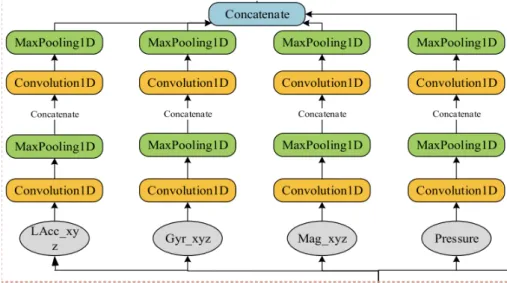
When implementing a CNN that uses multiple sensors as input, Qin et al. [28] developed a parallel CNN architecture for extracting features, that were fed into an LSTM network. Each sensor was processed by their own CNN and then concatenated together, as shown in Figure 9. The model was able to classify eight various modes of transport; stationary, walking, running, bicycling, taking bus, car, subway, and train with an accuracy of 98.1%.

Tambi et al. [25] proposed a different CNN architecture that utilized the data from the spectrogram of the accelerometer and gyroscope. This spectrogram showed the magnitudes of various frequencies present in specific time windows. These spectrograms were passed through two 1D convolutional layers and a single fully connected layer. Tambi et al. classified four modes of transport with an accuracy of 91%.

(30)

Figure 7: CNN architecture of Liang et. al. using accelerometer magnitude as input [7].

Figure 8: Single-channel CNN architecture of Han et al. fusing the 3 axis accelerom-eter into a single activation map [9].

Long Short Term Memory models in Transport Mode Detection

Long Short Term Memory (LSTM) models are types of Recurrent Neural Networks (RNN) that are neural networks that are used to process sequential data. Most commonly used in natural language processing or audio processing, they can also be applied to the problem of transport mode detection. LSTM networks have the capability of learning long term dependencies in the data, which is why they are suitable for the problem of transport mode detection. This is accomplished by having specific architectures, utilizing input gates, forget gates, and memory cells

(31)

Figure 9: CNN architecture of the multi-sensor feature extractor created by Qin et al. [28].

[41]. The LSTM models in transport mode detection either utilize many-to-one or many-to-many classification. In many-to-one classification, a window is split into multiple smaller time frames, and a final classification is made after the final frame is passed through the network. Each frame contains data from a specific time range and remembers specific features from that data. When multiple frames of data from a window are passed through the LSTM network, these specific features from previous frames are used when processing later frame. The final classification is made once all frames are passed through the LSTM. A diagram from Guvesan et al. [14], as shown in Figure 10, illustrates how these frames in windows are passed through the LSTM model. In many-to-many classification, the whole trip is taken into consideration and windows of a set time are continuously classified by the network until the trip ends. With many-to-many classification, longer time dependencies are found by the LSTM networks.

There are two conventional approaches in the literature in the implementations of LSTM networks for transport mode detection. In one approach, as discussed previously, features are extracted from the time and frequency domain from frames of a specific size. These features are the same that can be used in Random Forest models, as shown in Table2. In the case of Guvesan et al. windows containing 10 frames are used, with each frame containing data of 252 distinct features (padded with zeros to ensure the input space is in the size of a power of two). These features are calculated from the x, y, and z axes of the accelerometer, gyroscope, magnetometer, as well as their calculated magnitude, which results in 12 different signals. Twenty-one features are extracted from these 12 signals resulting in a total of 252 features. The optimal window size was found to be 12 seconds, meaning each frame is 1.2 seconds long. The research of Qin et al. [28] illustrates the second approach to use LSTMs in transport

(32)

Figure 10: Simple Long Short Term Memory architecture with features extracted from frames [14].

mode detection. In their research, instead of using handcrafted features from the data, they utilize convolutional layers to extract meaningful features from specific time windows. Instead of utilizing windows with a specified amount of frames, the classification happens continuously. In this case, long term patterns in the data can be observed, as the memory is not limited to the set windows as implemented by Guvesan et al. They argue that finding long term patterns in the data, such as how often a transport mode starts and stops, can be the difference between identifying a train or a metro. The combination of using CNNs for feature extraction and LSTMs to find temporal relations in the data is a CNN-LSTM model.

2.6 Creation of travel chains

This section focuses on the creation of travel chains from the outputs of models that researchers create. The process of creating travel chains from the output of these models is based on grouping of the windowed results into segments of a single transport mode of varying length. In this grouping of windows, errors made by the models can be fixed. Guvesan et al. [15] propose a "Healing" algorithm, a similar concept to what other researchers do for grouping. In this Healing algorithm, three different types of segments are classified, pedestrian, stationary, and transportation. Stationary periods are classified as stationary if they are right before or right after a pedestrian segment, or are in between transportation segments and the stationary period are 5 minutes or longer. After this, all the transportation segments use the windows within them and take the most common label. The results of this algorithm, as

(33)

shown in Figure11, update the wrongly classified bus windows to metro windows, as the majority of windows in the segment are labelled as a metro. The implementation of a healing algorithm on the outputs of the model can significantly improve results. Guvesan et al. show that their healing algorithm increased the overall recall of the transport modes by about 12%. However, for these healing algorithms to be practical, the prediction for walking and stationary must be high.

Figure 11: Healing algorithm of Guvesan et al. [15] where first row is the output of their model and the second row shows the changes made by the healing algorithm.

(34)

3 Real-world data and its characteristics

There are significant differences between synthetic lab generated data for transport mode detection and real-world data. Synthetic data is data that has a controlled process of collection, with a specific smartphone or sensor setup, which is constant for the collection of data. This type of data is common in transport mode detection research as it can be reproducible and produces a baseline goal that is the limit of what can be achieved with real-world data. In this section, the real-world data and the challenges it poses will be explained. With insights from the analysis of the issues with the real-world data, these issues can be addressed, and the accuracy results in the real world scenario can approach the results observed with controlled lab data.

3.1 Challenges with real world data

In data collection on real-world devices, errors can occur with the data collected from the sensors. The following subsections will explain these errors and how this research will attempt to address those errors.

Inconsistent sampling frequency

When collecting sensor data from various devices, different devices allow for different sampling frequencies. As well as when the sampling frequencies are set, they are not consistent over time, due to processes running on smartphone devices outside of the scope of data collection. For example, when another application is using up the computational resources of the smartphone in the foreground, the data collection application in the background can be impacted with a lower sampling frequency. On the other hand, if another application in the foreground is collecting the same sensor data as the data collection application for transport mode detection at a higher frequency, then the sampling frequency of the data collection application also increases. Therefore, in order to deal with the inconsistent sampling frequencies, the data will be downsampled or upsampled to a specified sampling frequency that could be achieved by the sensors and then linearly interpolated. In the case of upsampling the data, there might be a reduction of accuracy compared to the standard sampling frequency. However, this issue cannot be solved.

Inconsistent orientation of sensors in devices

When collecting sensor data from various devices, different users can store their phone in different orientations which causes the sensors to output different data for this

(35)

different orientation. Furthermore, different smartphone devices have the orientation of their motion-sensing chips in differing orientation. For example, Apple devices have the orientation of the z-axis sensors flipped in comparison to most Android devices. In order to deal with the inconsistent orientation of sensors, the data can be augmented by rotating the axis of the rotation dependent sensors and trained on the augmented data. Collecting data for training from a broad range of various devices from different manufacturers can also improve the generalization of the models on real-world data during inference.

Inconsistent location of devices

Different users of smartphones store their smartphones in different locations; in their pockets, hands, backpack, or purse. Different storage locations can cause the outputs of sensors to vary in noise and orientation, more so than when dealing with the inconsistent orientation of devices. In order to deal with the inconsistent orientation of devices, the only possible solution is to collect data with the smartphones stored in different locations. The more representative the training data, the better the generalization will be. Filtering of the sensor data might help with the generalization of the model for varying locations. However, this might lead to a loss of essential artefacts in the data and must be tested.

Inconsistent sensors in devices

Different smartphone devices used in transport mode detection have differing sets of sensors based on the models of devices; for example, some cheaper models of smartphones might not include a barometer in their sensor set. Furthermore, some sensors in cheaper devices can have lower quality and precision in the signals recorded. To fix issues with sensors of differing quality, the model should be trained on a wide array of sensors with these differing signal qualities, to achieve realistic results. In order to accommodate smartphone devices with various sets of sensors, various models can be built; of course, this can lead to a decrease in the accuracies of transport mode detection. Therefore, studying the achievable accuracies of models with different sensor sets is essential to understand the possibilities of implementations of transport mode detection on various devices.

Non-monotonous data from sensors

In real-world data collection due to the limited processing power of smartphones dealing with multiple processes, non-monotonous data collection can occur. This entails data from sensors arriving in inconsistent intervals, while at times being

(36)

unordered. In such cases, it is not possible to achieve real-time transportation mode detection. However, due to the nature o the problem, it is not necessary to process data in real-time. Therefore, it is not an issue when dealing with the processing of the sensor data at a later time. However, it is necessary to understand the limitations of transport mode detection and its implementations in real-time.

Inconsistent settings in data collection

Issues in transport mode detection arise when dealing with various users of these applications in various locations. The settings in which data is collected profoundly impact the signals that sensors produce. These settings are, for example, road or track conditions or different models of the vehicle used for transportation. For example, a car will produce vastly different sensor data when riding on a highway with constant velocity, where the signal appears to imply that the user is stationary, or when the car is riding on a dirt road with constant velocity, where the terrain of the road significantly impacts the sensor signal output. Some of these differences can be reduced through filtering of the signal. However, this filtering can remove specific artefacts in the data that can be used to differentiate between a car and a bus, for example, where a car and a bus on the highway will look more similar than a car on a highway and a car on a dirt road. The solutions to these problems lie with the data used in training. The more diverse and complete the training data is, the better it will perform in a real-world scenario. When dealing with transport mode detection in different countries, it is a good idea to create new training data for models specific to those regions if possible.

Data privacy concerns

When dealing with the data describing the daily movement of people, there are many issues with data privacy. The main issue is with tracking the exact location of users for 24 hours a day in order to monitor their transport mode use habits accurately. This information is very sensitive and contains information on where people live, work, and spend their time at exact times during the day. Due to the sensitivity of this data, many users do not accept the constant tracking of their locations for transport mode detection with GPS data. For this reason, research has been focused on using data from sensors such as accelerometers, gyroscopes, magnetometers, and barometers that are able to detect transport modes while simultaneously not containing as much personal data about the users. Some research, as described in the Background section of this thesis, uses sound data for transport mode detection. Sound data typically also contains a lot of sensitive user information, that many users might not be willing to share, for example, personal conversations. Therefore, this research will focus on transport mode detection using sensors that do not contain sensitive data to users; accelerometers, gyroscopes, magnetometers, and barometers.

(37)

4 Materials and Methods

This chapter proposes the methods used for collecting the data and explains the char-acteristics of the data set used for the training of the CNN. It provides explanations for the methods used in recreating state of the art models and their preprocessing techniques. It also proposes the methods used in optimizing the model architecture as well as selecting the optimal set of preprocessing techniques on the data, to achieve fast convergence of the model. Finally, the chapter will describe the technologies used to preprocess the data and train the CNN models.

4.1 Data

Data collection

Data collection is performed using a data collection application on smartphone devices, as shown in Figure12. This application allows users to collect all necessary sensor data for various modes of transportation at a specified frequency. The application works by the user pressing the transport mode buttons once a change in transport mode has been made. Every stop in the transportation mode, for example, a bus stopping at a bus stop requires the user to press the stationary button, and once the bus resumes travel and starts moving again, then the bus button is pressed again. The list of possible transport modes collected is:

• Stationary • Walk • Stairs • Run • Bicycle • Kickscooter • E-Kickscooter • Skateboard • Ice-Skate • Row-boat • Sailboat • Escalator • Elevator • Metro • Train • Tram • bus • Car • Electric car • Motorbike • Scooter • Airplane • Ferry • Motorboat

The application records the sensors that this research will use in transport mode detection; Accelerometer, Gyroscope, Magnetometer and Barometer. The Accelerom-eter, Gyroscope, and Magnetometer are mostly sampled at a frequency of 50Hz; some trips are recorded at 100Hz. The barometer is mostly sampled at 5 Hz; some trips are sampled at 1Hz or 10Hz. The data is collected in two different fashions, one for the training and one for testing. In the training data, each data file for training contains only one mode of transport along with stationary periods. In the testing data, whole travel chains are recorded. For the models of transport mode detection, only 10

(38)

Transport Mode Training Data Hours Testing Data Hours Car 102.8 6.9 Bus 37.3 8.4 E-Kickscooter 36.8 1.1 Airplane 28.4 5.4 Stationary 27.0 22.5 Metro 25.0 18.4 Train 24.2 13.4 Bicycle 17.9 1.4 Pedestrian 14.7 24.6 Tram 6.5 3.2

Table 4: Amounts of data in hours of each transportation mode in the training and testing data sets.

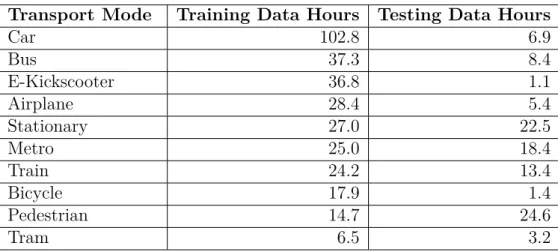
modes are taken into consideration due to the lack of data in other categories. The amounts of data of each mode, as shown in Table4, is collected by multiple users. Eight different users collect the training data on 17 devices, six different iPhone models and 11 different Android models. The testing data was collected by 12 users from 19 different device models, six different iPhone models and 13 different Android models. Due to the unbalanced nature of the dataset, the models will be trained on balanced batches of data. Therefore, data from classes with lower amounts of data will be replicated in each epoch.

Data splitting

The training data is used for the development and testing of the various data preprocessing techniques, data augmentation, and model architectures. It is split into a training set containing 80% of the data and a development set containing 20% of the data from the data collected for training, as shown in Table 4. Once an optimal model is selected using comparisons with the development set, it will be tested on the testing set, as shown in Table 4. The baseline CNN models will be trained and tested on the same data as the models proposed in this thesis, and a final comparison of the results will be made using the results of all these models on the testing data set.

Data prepossessing

The data was preprocessed in multiple stages, as described in the raw data processing section of the Background. First, the signal data is taken in and up-sampled or down-sampled to match 50Hz, then the data is windowed to the specified length.

(39)

Figure 12: Application used for the collection of transport data.

After this, if applicable, the specified filtering technique or gravity removal technique is applied to the windowed signal data. Finally, if applicable, the data is normalized using a specified normalization technique.

4.2 Evaluation metrics

In this research, the macro-averaged F1-score will be used to determine the success of these models as the purpose of transport mode detection requires both high recall and precision. The formula for precision, recall and F1 are described in Equations7,8, and9 where TP is the number of true positives, FP is the number of false positives,

(40)

and FN is the number of false negatives. P recision= T P T P +F P (7) Recall = T P T P +F N (8) F1 = 2∗ P recision∗Recall P recision+Recall (9)

The F1 score is calculated for each class and then the macro-averaged F1-score is calculated by taking the average of these F1-scores. In this thesis, for simplicity, the macro-averaged F1-score of the model is simply referred to as the F1-score of the model.

4.3 Baseline convolutional neural networks

This section will focus on how the various baseline convolutional neural network models will be trained and evaluated.

Convolutional Neural Network of Liang et al.

To implement the Convolutional Neural Network of Liang et al. [7] that has been discussed in the Background section, the data must be processed according to their methodology. In their method, the accelerometer signal is sampled at 50 Hz and windowed into windows of 10 seconds. The gravity is removed from the raw data using a low-pass filter at 0.8 Hz. After this, the data is smoothed using a Savitzky-Golay filter, and the magnitude of the acceleration is calculated by taking the root of the sum of the squares of the three axes of the accelerometer. Finally, the data is normalized using a z score normalization. The data is then used to train a CNN with seven convolutional and pooling layers with a Leaky ReLU as the activation function, followed by a fully connected layer.

Convolutional Neural Network of Han et al.

To implement the Convolutional Neural Network of Han et al. [9] that has been discussed in the Background section, the data must be processed according to their methodology. In their method, the accelerometer signal is sampled at 20 Hz and windowed into windows of 10 seconds. After this, the data is normalized using the Z