Institut für Algorithmen und Kognitive Systeme
Studienarbeit
Simulation in Computational Fluid Dynamics and parallel computing
(Simulation in der numerischen Strömungsmechanik und paralleles Rechnen)
Feng, Gu
Matrikelnumber: 1241252 SS 2007
Betreuer: Prof. Dr. J. Calmet (IAKS) Betreuende Mitarbeiter: Dr. Poehlmann (IAVF AG) Dr. Dienwiebel (IAVF AG)
Ich versichere, dass die vorliegende Arbeit—bis auf die offizielle Betreuung durch den Lehrstuhl—ohne fremde Hilfe von mir durchgefuehrt wurde.
Karlsruhe, den Juli, 2007 --- FENG, Gu
Acknowledgements
During my work, Dr. Poehlmann and Dr. Dienwiebel have answered many questions that occurred in the simulation, and all of the members in the team tribology by the firm IAVF AG have given me useful introductions when I am in difficulty.
Prof. Dr. J. Calmet (IAKS) has given me necessary advices and suggestions throughout the whole work.
Contents
Abstract...3
1 Motivation...5
1.1 CFD (Computational Fluid Dynamics) ...5
1.2 OpenFOAM (Open Field Operation and Manipulation)...5
2. Problems in the simulation and solutions...7
2.1 Dambreak...8
2.3 Variable description...9
2.4 Mesh generation...10
2.5 Non-uniform ...13
2.6 Tensor products define...16
2.7 Stream files for parallel computing ...17
2.8 New class defined...18
2.9 New solver...19
3 Model of two Cyclic Boxes ...21
3.1 The properties of the variable boundaries...22
3.2 Environmental elements define ...22
3.3 Meshes defined...23
3.4 Object boundaries ...24
3.5 Input of the real data...24
3.6 More complex models ...27
3.6.1 Problem 1 ... 28
3.6.2 Problem2 ... 28
4 Experiments results and explanation ...29
4.1 Visualization ...29
4.2 Simulations...31
4.2.2 Part2... 32
4.2.3 Part3... 33
4.3 Dynamic mesh ...34
5 Speedup ...35
5.1 Domain distribution thinks (MPI)...35
5.2 Time distribution thinks ...37
6 Other useful software ...39
7 Conclusions ...41
Figure list ...43
Program list ...45
Abstract
CFD (Computational Fluid Dynamics) is a technique that is widely used in industry and scientific research. One can study the different results between the simulation and the real experiments. By adjusting the model a more realistic description of the experiment can be achieved.
In this work open source software OpenFOAM (Open Field Operation and Manipulation (compiled by C++ under Linux)) is being used. For the specific needs of practical experiments, a method has to be developed to use surface data generated by AFM (Atomic Force Microscope) measurements. The physical model for the simulation will be set up and tested firstly in 2-Dimension, and then in 3-Dimension. Because of the large amount of the real data (1/4 M Pixel), the comparatively slow speeds of the simulation, alternative solutions of this problem have to be considered. Key words: CFD, OpenFOAM, real data, physical model, slow speeds.
In the following chapters OpenFOAM software will be introduced firstly, since we will use it as main tools in our simulations. This software is only in commercial use at its beginning design stage, and now it is open for all users. It is developed under the Linux operating system, uses C++ as its core technologies, the solvers and utilities are the important cases in this application; it compiles most equations of motion as its standard solvers.
And then we will recommend the data structures, which will be used in our simulation environments. In experiments we have got the nano-structure pictures of different material surfaces, and we should change them into databases that we could use in our simulation models. To explain this we also give the basic model that we will use in the object description.
In this work we observe only how the gravities of the environments and the distances between two surfaces will affect the object’s movements in our simulations.
To obtain the results of our simulations we have alternative methods in computing, that is, to get the description of the movements of objects in our simulations we have to calculate from the beginning status to the end situation ( here we use time as our simulation’s limitations, i.e.: 10 second, 120 second, 200 second…). MPI is a domain decomposition way, it takes place during the calculation; we can distribute our calculation in different computers, before we arrive at our aims.
1 Motivation
1.1 CFD (Computational Fluid Dynamics)
is one of the branches of fluid mechanics that uses numerical methods and algorithms to solve and analyze problems that involve fluid flows.
Here simulations from the beginning of experiments are running step by step to the aim condition, every movement is visible and capable of being stopped, all of the results can be observed separately.
1.2 OpenFOAM (Open Field Operation and Manipulation)
Is one open source software, the full name is “Open Field Operation and Manipulation”. It is useful in the simulation of complex fluid flows involving chemical reactions, turbulence and heat transfer, and solid dynamics, electromagnetics and the pricing of financial options, moreover the files and their structures are able to be changed.
The newest version of OpenFOAM is 1.4. It also supports the cygwin (allow various versions of Microsoft Windows to act somewhat like a UNIX system), but the speed is slower.
After unpacking the packages of the OpenFOAM, package gcc and java packages for the observation of simulations (using FoamX) should be installed:
Linux
Above 9.3 is in demand, and installation of additional new gcc package. Paraview
Third-party software to visualize the numeric simulation as it is in the real world. With different time steps, the simulation runs continually.
C++ modules
2. Problems in the simulation and solutions
The main files that should be modified in the simulation are:
setFieldDict, blockMeshDict, controlDict, and the files of beginning status in the ‘0’ time folder.
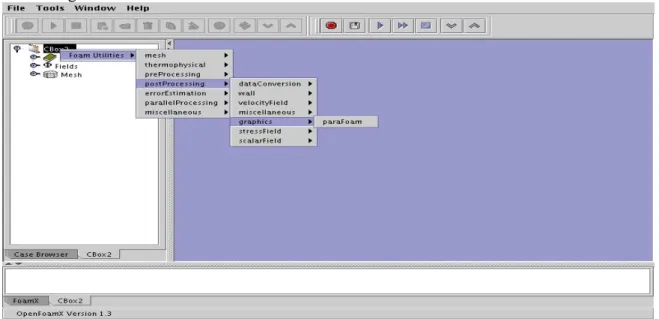
Generally for a physicist or a mechanist, one prefers to use the following faces of the FoamX:
Fig 1 Mainframe of the FoamX
2.1 Dambreak
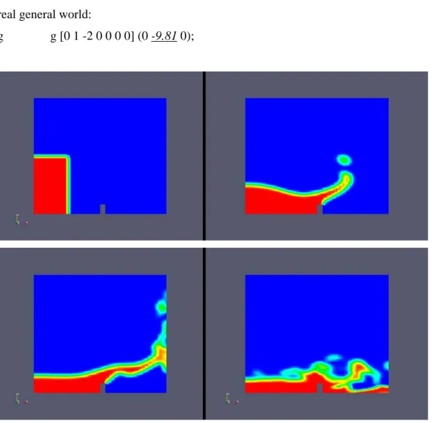
Set the “dambreak” as time = 1s and the gravity ‘-9.81’, i.e.: same situation as in the real general world:
g g [0 1 -2 0 0 0 0] (0 -9.81 0);
Fig 3 dambreak
This simulation describes how a volume of water falls down in one container.
2.2 The variables that are modified
I Variable modified Gamma FoamFile { version 2.0; format ascii; root "/root/OpenFOAM/feng-1.3/run/interFoam"; case "newmodell3_D2"; instance ""0""; local "";
class volScalarField; object gamma; } U FoamFile { version 2.0; format ascii; root "/home/feng_1.3/OpenFOAM/OpenFOAM-1.3/interFoam"; case "newmodell3_D2"; instance ""0""; local ""; class volVectorField; object U; } 2.3 Variable description IIVariable description
One subject can be described just with an original object. i.e.:
“A” as “wall”, so “A” can move and be turned around, it will have the properties of wall;
“A” can also be defined as “empty”, so there will be nothing in “A”, it is necessary for 2-D situations.
Gamma dimensions [0 0 0 0 0 0 0]; internalField uniform 0; boundaryField { movingWall { type zeroGradient; } leftrightWall { type cyclic; value uniform;
} frontAndBack { type empty; } } U dimensions [0 1 -1 0 0 0 0]; internalField uniform (0 0 0); boundaryField { leftWall { type fixedValue; value uniform (0 0 0); } rightWall { type fixedValue; value uniform (0 0 0); } lowerWall { type fixedValue; value uniform (0 0 0); } defaultFaces { type empty; } } 2.4 Mesh generation III Mesh generation version 2.1; `format' ascii; root ""; case ""; instance ""; local "";
class dictionary; object blockMeshDict;
// * * * * * * * * * * * * * * * * * * * * * * * * * * * * * * * * * * * * * // changecom(//)changequote([,])
define(calc, [esyscmd(perl -e 'printf ($1)')])
define(hex2D, hex ($1b $2b $3b $4b $1t $2t $3t $4t)) define(quad2D, ($1b $2b $2t $1t)) define(frontQuad, ($1t $2t $3t $4t)) define(backQuad, ($1b $4b $3b $2b)) convertToMeters 1; define(side, 10.0) define(height, 50.0) define(nrcellsx, 10) define(nrcellsy, 30) define(origox, 0.0) define(origoy, 0.0) define(coordinatesidex, calc(origox+side)) define(coordinatesidey, calc(origoy+height)) define(Z1, 0.0) define(Z2, 2.0) vertices ( (origox origoy Z1) (coordinatesidex origoy Z1) (coordinatesidex coordinatesidey Z1) (origox coordinatesidey Z1) (origox origoy Z2) (coordinatesidex origoy Z2) (coordinatesidex coordinatesidey Z2) (origox coordinatesidey Z2) ) blocks (
hex2D(a1, a2, a3, a4) (nrcellsx nrcellsy 2) simpleGrading (1 1 1) ); patches ( patch inlet ( quad2D(a1,a2) ) patch outlet ( quad2D(a3,a4) ) wall back ( backQuad(a1,a2,a3,a4) )
wall front ( frontQuad(a1,a2,a3,a4) ) wall wall ( quad2D(a1,a4) quad2D(a2,a3) ) ); Running results: // * * * * * * * * * * * * * * * * * * * * * * * * * * * * * * * * * * * * * // version 2.1; format ascii; root ""; case ""; instance ""; local ""; class dictionary; object blockMeshDict; // * * * * * * * * * * * * * * * * * * * * * * * * * * * * * * * * * * * * * // convertToMeters 1; vertices ( (0.0 0.0 0.0) (10 0.0 0.0) (10 50 0.0) (0.0 50 0.0) (0.0 0.0 2.0) (10 0.0 2.0) (10 50 2.0) (0.0 50 2.0) ) blocks ( // block0 hex (0 1 2 3 4 5 6 7) (10 30 2) simpleGrading (1 1 1) ); patches ( patch inlet ( (0 1 5 4)
) patch outlet ( (2 3 7 6) ) wall back ( (0 3 2 1) ) wall front ( (4 5 6 7) ) wall wall ( (0 3 7 4) (1 2 6 5) ) ); 2.5 Non-uniform
Definition: a non-uniform variable describes one type character that will be affected by outside forces into different values in one object, i.e.: one running water, the inside and outside velocities are not the same value (in fact, every point of one cube water has different velocity), so we can use the non-uniform to describe the velocity of this water; the shape of one object has the same theory, we can see the object’s changes, when we use non-uniform to define it.
The contra-side of the non-uniform is uniform, it can be simply set with stabile value, i.e.: the thickness of some medium.
There is also something that would be changed in one simulation, or could not be described with one same value in an object at the beginning of our simulation.
So it is useful introducing non-uniform, the shortcomings of it is that every part of an object have to be defined, it slows the speed of simulation because of more data to be controlled.
After the initializing of the simulation, the variable of U and Gamma will be set as non-uniform:
IV Non-uniform Gamma:
internalField uniform 0; boundaryField { leftWall { type zeroGradient; } rightWall { type zeroGradient; } lowerWall { type zeroGradient; } defaultFaces { type empty; } } U: dimensions [0 1 -1 0 0 0 0]; internalField uniform (0 0 0); boundaryField { leftWall { type fixedValue; value uniform (0 0 0); } rightWall { type fixedValue; value uniform (0 0 0); } lowerWall { type fixedValue; value uniform (0 0 0); } defaultFaces {
type empty; }
}
After the start-up: Gamma FoamFile { version 2.0; format ascii; root "/root/OpenFOAM/feng-1.3/run/interFoam"; case "newmodell3_D2"; instance ""0""; local ""; class volScalarField; object gamma; } // * * * * * * * * * * * * * * * * * * * * * * * * * * * * * * * * * * * * * // dimensions [0 0 0 0 0 0 0];
internalField nonuniform List<scalar> 3200 (1 1 ,,, ) U: FoamFile { version 2.0; format ascii; root "/root/OpenFOAM/feng-1.3/run/interFoam"; case "newmodell3_D2"; instance ""0""; local ""; class volVectorField; object U;
}
// * * * * * * * * * * * * * * * * * * * * * * * * * * * * * * * * * * * * * // dimensions [0 1 -1 0 0 0 0];
internalField nonuniform List<vector> 3200
( (0 0 0) ,,, )
2.6 Tensor products define V Tensor products define class vector { double V[4]; public: enum components { X, Y, Z, W }; vector(){}
vector(const double Vx, const double Vy, const double Vz, const double Vw) {
V[X] = Vx; V[Y] = Vy; V[Z] = Vz; V[W] = Vw; }
double& x() { return V[X]; } double& y() { return V[Y]; } double& z() { return V[Z]; } double& w() { return V[W]; }
const double& x() const { return V[X]; } const double& y() const { return V[Y]; } const double& z() const { return V[Z]; } const double& w() const { return V[W]; }
friend vector operator+(const vector& v1, const vector& v2) {
return vector(v1[X]+v2[X], v1[Y]+v2[Y], v1[Z]+v2[Z], v1[W]+v2[W]); }
. .
friend double operator&(const vector& v1, const vector& v2) {
return (v1[X]*v2[X] + v1[Y]*v2[Y] + v1[Z]*v2[Z]+ v1[W]*v2[W]); }
friend vector operator^(const vector& v1, const vector& v2) { return vector ( (v1[Y]*v2[Z] - v1[Z]*v2[Y]), (v1[Z]*v2[X] - v1[X]*v2[Z]), (v1[X]*v2[Y] - v1[Y]*v2[X]), (v1[Y]*v2[W] - v1[W]*v2[Y]), (v1[W]*v2[X] - v1[X]*v2[W]), (v1[W]*v2[Z] - v1[Z]*v2[W]) ); } };
2.7 Stream files for parallel computing VI Stream files for parallel computing
void Foam::lduAddressing::calcLosort() const { if (losortPtr_) { FatalErrorIn("lduAddressing::calcLosort() const") << "already be calculated" << abort(FatalError); } labelList nNbrOfFace(size(), 0);
const unallocLabelList& nbr = upperAddr(); forAll (nbr, nbrI)
{
nNbrOfFace[nbr[nbrI]]++; }
labelListList cellNbrFaces(size()); forAll (cellNbrFaces, cellI) { cellNbrFaces[cellI].setSize(nNbrOfFace[cellI]); } nNbrOfFace = 0; forAll (nbr, nbrI) { cellNbrFaces[nbr[nbrI]][nNbrOfFace[nbr[nbrI]]] = nbrI; nNbrOfFace[nbr[nbrI]]++; }
losortPtr_ = new labelList(nbr.size(), -1); labelList& lst = *losortPtr_;
label lstI = 0;
forAll (cellNbrFaces, cellI) {
const labelList& curNbr = cellNbrFaces[cellI]; forAll (curNbr, curNbrI)
{ lst[lstI] = curNbr[curNbrI]; lstI++; } } }
For the result of the friction, one should use new solvers: 2.8 New class defined
VII Class defined
#ifndef exampleClass_H #define exampleClass_H #include ".H" namespace Foam { class someClass; class exampleClass : public baseClassName { dataType data_; exampleClass(const exampleClass&); void operator=(const exampleClass&); public:
static const dataType staticData; exampleClass();
exampleClass(const dataType& data); exampleClass(Istream&);
exampleClass(const exampleClass&); static autoPtr New();
~exampleClass();
void operator=(const exampleClass&);
friend Istream& operator>>(Istream&, exampleClass&);
friend Ostream& operator<<(Ostream&, const exampleClass&); };
}
#include "exampleClassI.H" #endif
2.9 New solver VIII Solver myFoam.cfg dictionaries { include "$FOAMX_CONFIG/dictionaries/controlDict/controlDictAdjustTimeStep.cfg"; fvSchemes; fvSolution; include "$FOAMX_CONFIG/dictionaries/transportProperties/twoPhaseTransportProperties.c fg"; include "$FOAMX_CONFIG/dictionaries/environmentalProperties/environmentalPropertiesg .cfg"; include "$FOAMX_CONFIG/dictionaries/dynamicMeshDict/dynamicMeshDict.cfg"; } fields { include "$FOAMX_CONFIG/entries/geometricFields/pd.cfg"; include "$FOAMX_CONFIG/entries/geometricFields/U.cfg"; include "$FOAMX_CONFIG/entries/geometricFields/gamma.cfg"; } patchPhysicalTypes { include "$FOAMX_CONFIG/entries/patchPhysicalTypes/standard/patches.cfg"; include "$FOAMX_CONFIG/entries/patchPhysicalTypes/standard/meshMotion/patches.cfg"; wallContactAngle {
description "Wall boundary condition with specified contact-angle"; parentType wall; } } patchFieldsPhysicalTypes { gamma { include "$FOAMX_CONFIG/entries/patchPhysicalTypes/standard/gamma.cfg"; wallContactAngle gammaContactAngle; } U { include "$FOAMX_CONFIG/entries/patchPhysicalTypes/standard/U.cfg"; include "$FOAMX_CONFIG/entries/patchPhysicalTypes/standard/meshMotion/U.cfg"; } pd
{
include "$FOAMX_CONFIG/entries/patchPhysicalTypes/standard/pd.cfg"; }
3 Model of two Cyclic Boxes
After setting the model, the sum of the cells in dimension is equal to the actual number of the meshes.
The solvers that being used in the simulation:
2 incompressible fluids capture the interface using a VOF method. The cube used to set the object:
Fig 4 mesh model
Six sides of the block are defined with points (total 4) of the side.
wall movingWall ( (3 7 6 2) (1 5 4 0) ) wall leftrightWall ( (0 4 7 3)
(1 5 6 2) ) empty frontAndBack ( (0 3 2 1) (4 5 6 7) )
3.1 The properties of the variable boundaries IX The properties of the variable boundaries dimensions [0 0 0 0 0 0 0]; internalField uniform; boundaryField { movingWall { type zeroGradient; } leftrightWall { type cyclic; value uniform; } frontAndBack { type empty; } }
3.2 Environmental elements define X Environmental elements define FoamFile { version 2.0; format ascii; root "/root/OpenFOAM/feng-1.3/run/interFoam"; case "CBox2"; instance "constant"; local ""; class dictionary; object environmentalProperties; } // * * * * * * * * * * * * * * * * * * * * * * * * * * * * * * * * * * * * * // g g [0 1 -2 0 0 0 0] (0 -9.81 0); //as in the real general world
3.3 Meshes defined XI Meshes defined
convertToMeters 1; //conversion not be changed vertices ( (0 0 0) (50 0 0) (50 20 0) (0 20 0) (0 0 0.1) (50 0 0.1) (50 20 0.1) (0 20 0.1) ); blocks (
hex (0 1 2 3 4 5 6 7) (40 40 1) simpleGrading (1 1 1) //defined for 2-Dimension ); edges ( ); patches ( wall movingWall ( (3 7 6 2) (1 5 4 0) ) wall leftrightWall ( (0 4 7 3) (1 5 6 2) ) // wall bottomWall //( // (3 7 6 2) // (1 5 4 0) //) wall frontAndBack ( (0 3 2 1) (4 5 6 7) ) ); mergePatchPairs
( ); // ********************************************************************* **** // 3.4 Object boundaries XII Object boundaries movingWall { type wall; physicalType wall; nFaces 160; startFace 7840; } leftrightWall { type cyclic; physicalType cyclic; nFaces 160; startFace 8000; } frontAndBack { type wall; physicalType wall; nFaces 3200; startFace 8160; }
3.5 Input of the real data
In practice point ‘4’ and point ‘2’ are selected to set the whole box.
The statistics from AFM (Atom Force Microscope) can be grasped as surfaces pictures, firstly set them into statistics databank (i.e.: Excel, Access, FoxPro …), then be able to be used as original input.
Import the real data: XIII Input of the real data
int main(int argc, char *argv[])
{
char *ret1,*ret2,*ret3,*ret4,*ret5,*ret6;
char string1[200],string2[200],string3[200],string4[200],string5[200],string6[200]; FILE *Datei1,*Datei2, *Datei3,*Datei4,*Datei5,*Datei6,*Datei7;
if( (Datei1 = fopen("CBOXy.txt","r")) == NULL ) return -1;
if( (Datei2 = fopen("setFieldsDict","a+")) ==NULL) return -1;
if( (Datei3 = fopen("CBOXx.txt","r")) ==NULL) return -1;
if( (Datei4 = fopen("CBOXxcopy.txt","r")) ==NULL) return -1;
if( (Datei5 = fopen("CBOXy1.txt","r")) ==NULL) return -1;
if( (Datei6 = fopen("CBOXx1.txt","r")) ==NULL) return -1;
if( (Datei7 = fopen("CBOXx1copy.txt","r")) ==NULL) return -1;
ret1 = fgets(string1, 200, Datei1); ret2 = fgets(string2, 200, Datei3); ret3 = fgets(string3, 200, Datei4); ret2 = fgets(string2, 200, Datei3); ret5 = fgets(string4, 200, Datei5); ret4 = fgets(string5, 200, Datei6); ret4 = fgets(string5, 200, Datei6); ret6 = fgets(string6, 200, Datei7);
cout << “Datei2,"boxToCell{box (%s 0 0) (%s %s 0.3); fieldValues (volScalarFieldValue gamma 1 volVectorFieldValue U (0 0 0));} ",string3,string2,string1 “<<endl;
cout << “Datei2,"boxToCell{box (%s %s 0) (%s 20 0.3); fieldValues (volScalarFieldValue gamma 1 volVectorFieldValue U (100 0 0));} ",string6,string4,string5”<<endl;
while(ret1 != NULL && ret2 !=NULL) {
ret1 = fgets(string1, 200, Datei1); ret2 = fgets(string2, 200, Datei3); ret3 = fgets(string3, 200, Datei4); ret4 = fgets(string5, 200, Datei6); ret5 = fgets(string4, 200, Datei5); ret6 = fgets(string6, 200, Datei7);
cout << “Datei2,"boxToCell{box (%s 0 0) (%s %s 0.3); fieldValues (volScalarFieldValue gamma 1 volVectorFieldValue U (0 0 0));} ",string3,string2,string1”<< endl;
cout << “Datei2,"boxToCell{box (%s %s 0) (%s 20 0.3); fieldValues (volScalarFieldValue gamma 1 volVectorFieldValue U (100 0 0));} ",string6,string4,string5” <<endl;
}
fclose(Datei1); fclose(Datei2); fclose(Datei3); fclose(Datei4);
fclose(Datei5); fclose(Datei6); fclose(Datei7); return 0; }
Results of the input data from AFM: Setfields: FoamFile { version 2.0; format ascii; root "/root/OpenFOAM/feng-1.3/run/interFoam"; case "2phaseBox"; instance "system"; local ""; class dictionary; object setFieldsDict; } // * * * * * * * * * * * * * * * * * * * * * * * * * * * * * * * * * * * * * // defaultFieldValues ( volScalarFieldValue gamma 0 volVectorFieldValue U (0 0 0) ); regions ( boxToCell{box (0 0 0) (0.1 7.19 0.3); fieldValues
(volScalarFieldValue gamma 1 volVectorFieldValue U (0 0 0));} boxToCell{box (0
12.68 0) (0.1
20 0.3); fieldValues
(volScalarFieldValue gamma 1 volVectorFieldValue U (10 0 0));} boxToCell{box (0.1
0 0) (0.2 7.32
0.3); fieldValues
(volScalarFieldValue gamma 1 volVectorFieldValue U (0 0 0));} boxToCell{box (0.1
12.45 0) (0.2
20 0.3); fieldValues
(volScalarFieldValue gamma 1 volVectorFieldValue U (10 0 0));}
,,,,,,
boxToCell{box (49.93 17
0) (50
20 0.3); fieldValues
(volScalarFieldValue gamma 1 volVectorFieldValue U (10 0 0));} boxToCell{box (50
0 0) (50 1
0.3); fieldValues
(volScalarFieldValue gamma 1 volVectorFieldValue U (0 0 0));} boxToCell{box (50
17 0) (50
20 0.3); fieldValues
(volScalarFieldValue gamma 1 volVectorFieldValue U (10 0 0));} );
3.6 More complex models
There are many descriptions for one physical model, i.e.: the point number of the model can be changed, the result will occur other ways.
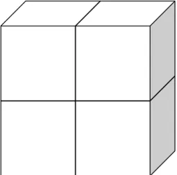
There are also more complex models for mesh generation, i.e.: dividing the above model into four pieces, defining this model for more complex situations:
Fig 5 mesh structure
3.6.1 Problem 1
The simulation can also be supposed to be made simpler in the pre-process: the cells of the object need firstly to be defined, and then continue other steps.
Because of the same beginning work, the data can be saved in one folder, so it will be more practical to observe the differences among them.
3.6.2 Problem2
With more and more simulations running in parallel, the data will be enlarged, some of the information at the beginning stage could be deleted, since every step of the simulation comes from the nearest step (i.e.: at 100s time-point, the data of 99.5s are in demand)
4 Experiments results and explanation 4.1 Visualization
Observing the simulation:
Fig 6 mainframe
Fig 8 in 2-D
Fig 9 in 3-D
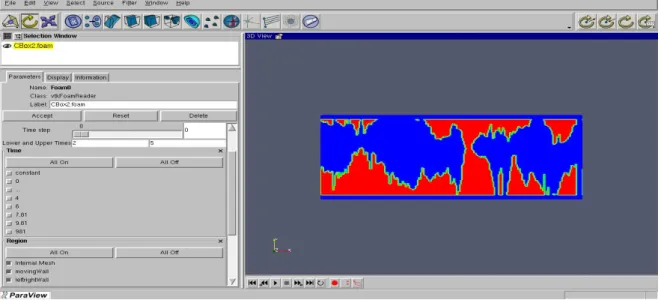
Paraview is separated from OpenFOAM, and injected in OpenFOAM while installation.
With command “paraview”, or the graphic menu in FoamX, it is visible.
Paraview will select “0” as the beginning state. For every 0.5 second there is a situation being saved, the simulation is discrete.
“Time step” in “control dictionary” could be modified to get more detailed results; the simulation would run more slowly because of the increased data.
y
ore ordentlich because of the hardness in
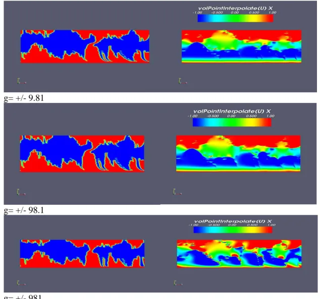
4.2 Simulations
ith the different gravity of two surfaces, the gravity will influence the iction between the two surfaces.
Fig 11 Beginning
g= +/- 0,000001
Fig 10 velocit
With more gravity, the end situation looks m two surfaces. 4.2.1 Part1 Simulations w fr Simulations
g= +/- 9.81
ng results
and the distance between the two surfaces :
The whole distance of our box, and the thicknesses of the two objects, using them to calculate the distance between the two surfaces.
i.e.: the whole box is 50m, the thicknesses of the two surfaces are 20m and 15m, so the distance between them is 15m.
Different distances with the same gravity: g= +/- 98.1
g= +/- 981
Fig 12 Runni
4.2.2 Part2
The gravity is one reason for the friction, can also affect it.
Fig 13 different distances
4.2.3 Part3
Sometimes the simulation becomes more complex and slowly because of the huge amount of data, even not be cable of running, typically in 3-D situation.
There is a connection between the simulation and the physical properties of the two en the rho number is below 2.1, the simulation can not further run:
phase2 { transportModel Newtonian; rho rho [1 -3 0 0 0 0 0] 2.075; nu nu [0 2 -1 0 0 0 0] 0.000148; phase2 { transportModel Newtonian; rho rho [1 -3 0 0 0 0 0] 2.05; nu nu [0 2 -1 0 0 0 0] 0.000148; simulation OK phase2 { transportModel Newtonian; rho [1 -3 0 0 0 0 0] 2.1; nu nu [0 2 -1 0 0 0 0] 0.000148; phase2 { transportModel Newtonian; rho rho [1 -3 0 0 0 0 0] 2.5; nu nu [0 2 -1 0 0 0 0] 0.000148; phase2 { transportModel Newtonian; surfaces, wh rho
rho rho [1 -3 0 0 0 0 0] 1000; nu nu [0 2 -1 0 0 0 0] 0.000148; Following picture shows this phenomenon:
Fig 14 out of running
t this time, all the elements of the objects run in different dimensions, they can not e described in an ordinary form; more computing is needed, the computer can not
t in the simulation process, the shape A
b
bear this.
4.3 Dynamic mesh
When the mesh needs to be changed after running, dynamic mesh is to be introduced to solve this problem. Dynamic mesh means tha
5 Speedup
MPI (Message Passing Interface): Only one time running:
Mean and max Courant Numbers = 0.042933758 0.47573913
l = 0.00047600522, Final residual = 1.1949953e-11, No 42 Min(gamma) = -1.8178472e-21 Max(gamma)
= 47210557, Final residual = 1.1840165e-11, No
Iterations 2 Liquid phase volume fraction = 0.44781442 Min(gamma) = -1.8024989e-21 Max(gamma) : Solving for gamma, Initial residual = 0.00046821087, Final residual = 1.1671876e-11, No ations 2 Liquid phase volume fraction = 0.44781442 Min(gamma) = -1.7865478e-21 Max(gamma)
residual = 0.00046427957, Final residual = 1.1549317e-11, No 4781442 Min(gamma) = -1.7699753e-21 Max(gamma)
724, Final residual = 9.3436951e-11, No
Ite 0.0021645826, Final residual = 9.9045951e-11,
No Iterations 679 ICCG: Solving for pd, Initial residual = 0.0008772519, Final residual = 9.4844974e-ations 680 time step continuity errors : sum local = 3.6185862e-13, global = -1.7846633e-20, e = -1.0932287e-18
e = 19914 s deltaT = 0.0013067151 Time = 2
BICCG: Solving for gamma, Initial residua Iterations 2 Liquid phase volume fraction = 0.447814
1 BICCG: Solving for gamma, Initial residual = 0.000 = 1 BICCG
Iter
= 1 BICCG: Solving for gamma, Initial Iterations 2 Liquid phase volume fraction = 0.4 = 1 ICCG: Solving for pd, Initial residual = 0.046027
rations 688 ICCG: Solving for pd, Initial residual = 11, No Iter
ulativ cum
ExecutionTime = 19314.49 s ClockTim 19914s/3600 = 5.5 h
5.1 Domain distribution thinks (MPI)
It distributes the simulation averagely in different computers; the calculating tasks in every computer are smaller.
This method uses the LAM command under Linux, one host computer and many
z directions N= (2,2,1)
nx x ny = Anzahle von Subdomain
n-1<PID> ssi:boot:base:linear: finished lamhalt –d
mpirun – np 4 interFoam $FOAM_RUN/interFoam Cbox2 –parallel < /dev/null >& log &
paraFoam $FOAM_RUN/interFoam/ Cbox2 processor1
Using MPI of four processors, the speedup is not four times as the one processor, the cause of it is that the costs of the communication of the four processors.
It depends not only on the processors being used, but also the running simulations themselves. That is, if the simulation need more communication when it is distributed, it will need more time by more processors, so the effects of the MPI is defected.
No of CPUs CPU time to convergence Speedup (maximal 255) computers. • LAM/MPI x, y and hostname > $FOAM_RUN/interFoam/Cbox2/system/machines lamboot -v $FOAM_RUN/interFoam/ Cbox2/system/machines n-1<PID> ssi:boot:base:linear: booting n0 (<MBT0>)
1 35620.4 s /3600s/h=9.9h 1.00
2 22398.8 s/3600 s/h =6.2h 1.60
4 11406.6 s/3600 s/h =3.2h 3.10
8 4247.32 s/3600 s/h =1.2h 8.88
To get the correct results the computers have to communicate with each other because tion at every second, the relation among intra-ne shortcoming of this method.
5.2 Time distribution thinks
The middle data of one simulation can be saved, making the simulation as assembly line.
Cause: there are discrete data in every step, for example: 0 second, 0.5 second, 1.0 second … so you can save them in one local computer, and then distribute them to other computers.
he same theory for other simulations, different simulations can be run at the same
pay off the time because of the communications. of running the same one simula
computers is close; it is o
T
time in different computers.
Shortcomings: not efficient for one simulation.
Hardware testing and software testing are being run between one multimedia computer and one general computer. MPI requires all computers the near qualities; otherwise the host should
6 Other useful software
They are better in some fields, for example, in the mesh generation (SALOME, NETGEN), or CAE-Linux can use the simulation direct from a real object:
(CAE-Linux)
(Salome)
7 Conclusions
The restrictions in simulation are difficult to be defined similarly as the real experiments; and the practical experiments needs more time than the simulations, since the simulations are only in one ideal world (it is actually one mathematical world).
Data from AFM (Atom Force Microscope) is greater than the bear of a usual computer; MPI methods are suggested to be used in the calculations to solve this problem; the two factors that affect the friction of the two surfaces greatly are the gravity of the environment and the distance between them.
For a computer scientist, the addition of mechanics and physics, sometimes the cooperation with different fields, are in demand.
In the future the new solvers for friction measurement and more variables in the real world are required.
Dimensions: [0 1 2 3 4 5 6 ]
No. Property Unit Symbol
al knowledge
1 Mass kilogram k
2 Length meter m
3 Time second s
4 Temperature Kelvin K
5 Quantity moles mol
6 Current ampere A
7 Luminous intensity candela cd
Interesting works will also be supposed in following fields:
• The stress field between one raising moving surface and one constant surface:
• efficiency in parallel communication • linear equation solver work
Figure list ...28 ...30 Fig 9 in 3-D...30 Fig 10 velocity ...31 Fig 11 Beginning...31 Fig 12 unning ... ... ...32 Fig 13 fferent di ... ... ...33 Fig 1 t of ... ... ...34
Fig 1 Mainframe of the FoamX ...7
Fig 2 Case selecting menu ...7
Fig 3 dambreak ...8
Fig 4 mesh model...21
Fig 5 mesh structure... Fig 6 mainframe ...29
Fig 7 function button...29 Fig 8 in 2-D....
R results ... ... ...
di stances.... ... ...
Program list
I Variable modified ...8
II Variable description ...9
III Mesh generation...10
IV Non-uniform ...13
V Tensor products define...16
VI Stream files for parallel computing ...17
VII Class defined ...18
VIII Solver ...19
IX The properties of the variable boundaries ...22
X Environmental elements define...22
XI Meshes defined ...23
XII Object boundaries...24
References
Germany
• Computational methods for fluid dynamics / J. H. Ferziger ; M. Peric, 1996
• C++ for business programming / John C. Mulluzzo, 2006
OpenFOAM community • ZIB • IAVF AG
• “Fundamental wear mechanism of metals”, M. Scherge, D. Shakhvorostov, K. Pöhlmann. IAVF Antriebstechnik AG, Im Schlehert 32, D-76187 Karlsruhe,
• Parallel computational fluid dynamics/ Wilders, P., 2002
• Turbomachinery design using CFD, 1994
• Computational fluid dynamics / T. J. Chung., 2002
• Biological micro- and nanotribology / Scherge, Matthias, 2001
• [GNU C++ for Linux] Tom Swan's GNU C++ for Linux / Tom Swan 2000
• C, C++ / Ulrich Kaiser ; Christoph Kecher, 2005