Theses
Thesis/Dissertation Collections
8-2017
Understanding High Resolution Aerial Imagery
Using Computer Vision Techniques
Fan Wang
[email protected]Follow this and additional works at:
http://scholarworks.rit.edu/theses
This Dissertation is brought to you for free and open access by the Thesis/Dissertation Collections at RIT Scholar Works. It has been accepted for inclusion in Theses by an authorized administrator of RIT Scholar Works. For more information, please [email protected].
Recommended Citation
Wang, Fan, "Understanding High Resolution Aerial Imagery Using Computer Vision Techniques" (2017). Thesis. Rochester Institute of Technology. Accessed from
by
Fan Wang
B.S. Harbin Institute of Technology, 2010 M.S. Harbin Institute of Technology, 2012
A dissertation submitted in partial fulfillment of the requirements for the degree of Doctor of Philosophy in the Chester F. Carlson Center for Imaging Science
College of Science
Rochester Institute of Technology August, 2017
Signature of the Author
Accepted by
ROCHESTER INSTITUTE OF TECHNOLOGY ROCHESTER, NEW YORK
CERTIFICATE OF APPROVAL
Ph.D. DEGREE DISSERTATION
The Ph.D. Degree Dissertation of Fan Wang has been examined and approved by the dissertation committee as satisfactory for the
dissertation required for the Ph.D. degree in Imaging Science
Dr. John P. Kerekes, Dissertation Advisor
Dr. Pengcheng Shi
Dr. Carl Salvaggio
Dr. Yandong Wang
Date
by Fan Wang Submitted to the
Chester F. Carlson Center for Imaging Science in partial fulfillment of the requirements
for the Doctor of Philosophy Degree at the Rochester Institute of Technology
Abstract
Computer vision can make important contributions to the analysis of remote sensing satellite or aerial imagery. However, the resolution of early satellite imagery was not sufficient to provide useful spatial features. The situation is changing with the advent of very-high-spatial-resolution (VHR) imaging sensors. This change makes it possible to use computer vision techniques to perform analysis of man-made structures. Meanwhile, the development of multi-view imaging techniques allows the generation of accurate point clouds as ancillary knowledge.
This dissertation aims at developing computer vision and machine learning algorithms for high resolution aerial imagery analysis in the context of application problems including debris detection, building detection and roof condition assessment. High resolution aerial imagery and point clouds were provided by Pictometry International for this study.
Debris detection after natural disasters such as tornadoes, hurricanes or tsunamis, is needed for effective debris removal and allocation of limited resources. Significant advances in aerial image acquisition have greatly enabled the possibilities for rapid and automated detection of debris. In this dissertation, a robust debris detection algorithm is proposed. Large scale aerial images are partitioned into homogeneous regions by interactive segmen-tation. Debris areas are identified based on extracted texture features.
Robust building detection is another important part of high resolution aerial imagery understanding. This dissertation develops a 3D scene classification algorithm for building
detection using point clouds derived from multi-view imagery. Point clouds are divided into point clusters using Euclidean clustering. Individual point clusters are identified based on extracted spectral and 3D structural features.
The inspection of roof condition is an important step in damage claim processing in the insurance industry. Automated roof condition assessment from remotely sensed im-ages is proposed in this dissertation. Initially, texture classification and a bag-of-words model were applied to assess the roof condition using features derived from the whole rooftop. However, considering the complexity of residential rooftop, a more sophisticated method is proposed to divide the task into two stages: 1) roof segmentation, followed by 2) classification of segmented roof regions. Deep learning techniques are investigated for both segmentation and classification. A deep learned feature is proposed and applied in a region merging segmentation algorithm. A fine-tuned deep network is adopted for roof segment classification and found to achieve higher accuracy than traditional methods using hand-crafted features.
Contributions of this study include the development of algorithms for debris detection using 2D images and building detection using 3D point clouds. For roof condition assess-ment, the solutions to this problem are explored in two directions: features derived from the whole rooftop and features extracted from each roof segments. Through our research, roof segmentation followed by segments classification was found to be a more promising method and the workflow processing developed and tested. Deep learning techniques are also investigated for both roof segmentation and segments classification. More unsuper-vised feature extraction techniques using deep learning can be explored in future work.
Kerekes, for the help, support and guidance of my research. You are a great advisor in balancing guidance and giving me the freedom to various projects of my interest. I cannot reach this point without your mentoring.
Besides my advisor, I would like to thank the rest of my thesis committee: Dr. Pengcheng Shi, Dr. Carl Salvaggio and Dr. Yandong Wang, for taking time to provide insightful comments and valuable advice.
In addition, there are several individuals I would like to express my appreciation. First, besides Dr. Yandong Wang, I would like to thank Frank Giuffrida, Stephen Schultz and Charles Mondello from Pictometry International Corporation for their guidance and dis-cussion in completing these projects. Also I would like to thank Dr. Harvey Rhody and Michael Richardson for their help and useful suggestions for my projects. A special thank to Sue Chan, Cindy Schultz and Beth Lockwood for their help and keeping things well orga-nized. I also wish to thank my friends: Bo Ding, Ming Li, Can Jin, Chao Zhang, Gajendra J. Katuwal, Zhaoyu Cui, Xuewen Zhang, Zhenlin Xu and Runchen Zhao for their help and companion. Last but not least, I want to devote my gratitude to my girlfriend Zhuoyi Xu and my family. Thank you for your unconditional support and encouragement in my life and study.
List of Tables ix
List of Figures x
1 Introduction 1
2 Objectives 3
3 Background 5
3.1 High Resolution Remotely Sensed Imagery . . . 5
3.2 A ‘Brief’ History of Computer Vision . . . 8
3.3 Computer Vision in Remote Sensing . . . 9
3.4 Deep Learning in Remote Sensing. . . 10
4 Debris Detection 12 4.1 Previous Research . . . 12
4.2 Approach . . . 13
4.2.1 Data . . . 14
4.2.2 Statistical and frequency analysis of debris area . . . 14
4.2.3 FFT based debris detection algorithm . . . 16
4.2.4 Object based debris detection algorithm . . . 17
4.3 Results. . . 23
4.3.1 FFT based debris detection algorithm . . . 23
4.3.2 OBIA debris detection algorithm . . . 23
4.4 Conclusion. . . 30
5 Building Detection 31
5.1 Previous Research . . . 31
5.2 Approach . . . 32
5.2.1 Data . . . 32
5.2.2 Simple algorithm exploration . . . 33
5.2.3 Robust building detection using computer vision technique. . . 35
5.3 Results. . . 40
5.3.1 Simple algorithm exploration . . . 40
5.3.2 Robust building detection using machine learning technique . . . 40
5.4 Conclusion. . . 43
6 Roof Condition Assessment 44 6.1 Previous Research . . . 44
6.2 Preliminary roof condition assessment . . . 46
6.2.1 Approach . . . 46 6.2.2 Results . . . 52 6.2.3 Conclusion . . . 54 6.3 Roof Segmentation . . . 54 6.3.1 Approach . . . 54 6.3.2 Results . . . 60 6.3.3 Conclusion . . . 68
6.4 Roof Segment Classification . . . 68
6.4.1 Approach . . . 68
6.4.2 Results . . . 75
6.4.3 Conclusion . . . 78
7 Summary and Future Work 80 7.1 Debris detection . . . 80
7.2 Building detection . . . 80
7.3 Roof condition assessment . . . 81
7.3.1 Preliminary roof condition assessment . . . 81
7.3.2 Roof segmentation . . . 81
7.3.3 Roof segment classification . . . 82
3.1 Comparison of Spatial Resolution of Commercial Satellite and Aerial Images 7
4.1 Data Sets Provided by Pictometry International for Debris Detection . . . . 14
4.2 Mean and Standard Deviation (Std) Values of Before-and-After Hurricane Ike Subimages. . . 15
6.1 Results of Texture Classification . . . 52
6.2 Result of Texture Classification without Feature Selection . . . 53
6.3 Result of BoW . . . 53
6.4 Confusion Matrix for Roof Segments Classification via ResNet . . . 76
6.5 Confusion Matrix for Roof Segments Classification via Traditional Method . 76
3.1 Comparison of commercial satellite and aerial images. . . 11
4.1 Before-and-After hurricane Ike images . . . 15
4.2 Before-and-After hurricane Ike images . . . 16
4.3 Fourier spectrum of no-debris and debris area . . . 16
4.4 Fourier spectrum of no-debris and debris area . . . 17
4.5 Fourier spectrum analysis . . . 18
4.6 Framework of OBIA debris detection . . . 18
4.7 Segmentation result with Scale Level 25 and Merge Level 99.7 . . . 19
4.8 Texture feature calculation. . . 20
4.9 Attribute image of texture range . . . 20
4.10 Attribute image of texture mean . . . 21
4.11 Attribute image of texture entropy (R band). . . 21
4.12 Attribute image of texture variance . . . 21
4.13 Attribute images of texture range with different kernel sizes . . . 22
4.14 Attribute images of texture variance with different kernel sizes. . . 22
4.15 FFT based debris detection Result . . . 23
4.16 OBIA based debris detection Framework . . . 25
4.17 OBIA based debris detection result . . . 26
4.18 Robust experiment on large scale image 1 . . . 27
4.19 Robust experiment on large scale image 2 . . . 28
4.20 Robust experiment on large scale image 3 . . . 29
5.1 Point cloud provided by Pictometry International . . . 33
5.2 Image provided by Pictometry International . . . 33
5.3 Detail of point cloud . . . 34
5.4 Large scale scene of point cloud . . . 34
5.5 Point cloud before and after outlier removal withk= 50 . . . 36
5.6 Plane model segmentation result . . . 37
5.7 Leftover after plane model segmentation . . . 37
5.8 DoN classification result . . . 38
5.9 Segmentation and feature extraction . . . 38
5.10 Feature extraction . . . 39
5.11 SVM classifier training and testing . . . 39
5.12 Framework of proposed simple algorithm . . . 41
5.13 Final result of our simple algorithm. . . 42
5.14 Data sample which RANSAC can not detect the main ground . . . 42
6.1 Classification of damage to masonry buildings [1] . . . 45
6.2 Manual data extraction . . . 47
6.3 Pictometry rooftop sample images . . . 48
6.4 Intact rooftop sample images with high within-class diversity . . . 49
6.5 Damaged rooftop sample images with tiny missing shingles. . . 49
6.6 Traditional texture features based classification framework . . . 50
6.7 Traditional texture feature computation . . . 50
6.8 Recursive feature elimination . . . 51
6.9 BoW framework . . . 51
6.10 Examples of HED side outputs on roof image : (a) original image, (b) HED side output 1, (c) HED side output 2, (d) HED side output 3, (e) HED side output 4. . . 56
6.11 Framework of self-tuning segmentation algorithm. . . 59
6.12 Typical impaired roof. . . 60
6.13 SLIC Superpixel result. . . 61
6.14 Pre and post-region-merging results. . . 62
6.15 Segmentation results by human, proposed algorithms and CTM: (a) original image, (b) human segmentation, (c) proposed algorithm, (d) CTM Result. . 64
6.16 Failure cases. . . 67
6.17 Labeled roof segment images. . . 69
6.19 Features for tree, debris, window, chimney, structure and ridge segments . . 72
6.20 Training data augmentation: (a) original roof image, (b) roof segments with background (c) resized segments after horizontal and vertical flipping. . . . 74
6.21 Examples of intact segments which are correctly classified by ResNet: (a)-(c) large intact roof segments, (d)-(e) small intact roof segments. . . 77
6.22 Examples of impaired segments which are correctly classified by ResNet: (a)-(b) large impaired roof segments, (c)-(d) small impaired roof segments. . 77
6.23 Examples of intact segments which are misclassified as impaired segments by ResNet: (a) large intact roof segments, (b)-(d) small intact roof segments. 77
6.24 Examples of impaired segments which are misclassified as intact segments by ResNet: (a) large impaired roof segments, (b)-(d) small impaired roof segments. . . 78
Introduction
High resolution aerial imagery contains plenty of information which is not able to be directly understood by a computer while it can be easily understood by the human vision system. Since computer vision aims to model, duplicate and exceed the abilities of human vision system through electrical hardware and computational models [2], it can make important contributions to the analysis of remote sensing or aerial imagery [3].
However, the resolution of early satellite imagery was not sufficient to provide useful spatial features [4]. For example, the spatial resolution of Landsat 7 (panchromatic band) is 15 m. Its pixel size is bigger than the size of many man-made or natural objects. Thus, pixel based or even sub-pixel based methods are the main trend of image analysis techniques in traditional remote sensing [5].
The situation is changing with the advent of very-high-resolution (VHR) imaging sen-sors [3]. The change makes it possible to use computer vision techniques to analyze of man-made structures. Meanwhile, the development of multi-view imaging techniques al-lows the generation of accurate point clouds as ancillary knowledge for analysis [3].
This dissertation aims at developing computer vision and machine learning algorithms for high resolution aerial imagery analysis in the context of application problems including debris detection, building detection and roof condition assessment. High resolution aerial imagery and point clouds were provided by Pictometry International for this study.
Debris detection after natural disasters such as tornadoes, hurricanes or tsunamis, is needed for effective debris removal and allocation of limited resources. It can be performed manually, but such effort is labor intensive and hinders the quick response needed in large hurricane impact zones. Significant advances in aerial image acquisition have greatly
promoted the possibilities for rapid and automated detection of debris. In this dissertation, a robust debris detection algorithm using texture features of debris areas is proposed.
Robust building detection is an important part of high resolution aerial imagery un-derstanding [6]. It also serves as pre-processing for building modeling and roof condition assessment. This dissertation develops a 3D scene classification algorithm for building detection using point clouds derived from multi-view imagery.
The inspection of roof condition is an important step of damage claim processing in the insurance industry. Currently, roof inspections are done by humans and are an expensive, time-consuming and unsafe process. Thus, automated roof condition assessment from remotely sensed images is proposed in this dissertation. Initially, texture classification and bag-of-words models are developed to assess the roof condition using features covering the whole rooftop. However, considering the complexity of residential rooftops, a more sophisticated method is proposed to divide the task into two stages: 1) roof segmentation, followed by 2) classification of the segmented roof regions. Deep learning techniques are investigated for both segmentation and classification. A deep learned feature is proposed and applied in the region merging segmentation algorithm. A fine-tuned deep network is adopted for roof segments classification and compared to traditional method using hand-crafted features.
The rest of this dissertation is organized as follows. Chapter 2 briefly states the ob-jectives of this research, and relevant background is reviewed in Chapter 3. The approach and results of debris detection, building detection and roof condition assessment are stated in Chapters 4, 5 and 6, separately. Finally, a summary and recommendations for future work are presented in Chapter 7.
Objectives
The purpose of this research is to develop computer vision and machine learning algorithms for understanding high resolution aerial imagery. More specifically, the objectives can be divided into three parts based on the applications:
• To investigate methods for debris detection using very-high-resolution (VHR) aerial images provided by Pictometry;
• To develop algorithms for 3D point cloud classification. The point clouds used are derived from multiple high resolution aerial images. The ultimate goal is to divide the scene into three categories: vegetative areas, terrain and building footprints; • To investigate automated roof condition assessment techniques using VHR aerial
imagery. The assessment includes preliminary roof condition assessment, roof seg-mentation and roof segments classification.
This study makes contributions to the use of computer vision and machine learning techniques to understand high resolution aerial imagery in the context of debris detection, building detection and roof condition assessment. An algorithm for debris detection is proposed and tested on large scale data. Building detection algorithms are developed using 3D structure features. The possibility is explored to assess the roof condition using features covered the whole rooftop image or features inside each roof segments. Algorithms for preliminary roof condition assessment, roof segmentation and roof segments classification are proposed and developed. Deep learning techniques are investigated for roof condition
assessment. As a fixed feature extractor, a deep learned feature is proposed for region representation in the roof segmentation. For roof segments classification, both traditional method using hand-crafted features and deep learning method are investigated. Fine-tuning a pre-trained deep network is used for roof segments classification and achieves better result than traditional method.
Background
In this chapter, the background of our research is reviewed. Section3.1reviews the devel-opment of high resolution remotely sensed imagery. A brief history of computer vision is stated. Computer vision and deep learning applied in remote sensing are described in the following sections.
3.1
High Resolution Remotely Sensed Imagery
The first moderate-resolution civilian earth observation satellite, Landsat 1, was launched in July 1972 as a new way of monitoring land cover and land use globally [7]. It carried the Multispectral Scanner System (MSS) with a spatial resolution of 80 m. The spatial resolution number specifies the ground distance covered by one pixel in the image.
In 1999, Landsat 7 was successfully launched which contained the Enhanced Thematic Mapper Plus (ETM+) with a 15 m panchromatic band and 30 m multispectral bands. Each pixel in a Landsat 7 image may represent an area as large as a house. The resolution is too coarse to be useful for analysis of a particular man made object of interest. Thus, image analysis techniques for Landsat 7 imagery are confined to pixel-based analysis or even sub-pixel analysis and the applications are limited to land use and land cover classification. The spatial resolution of these early satellite images were not sufficient to identify useful spatial features. This situation is changing with the increasing spatial resolution of new generation sensors such as SPOT 5, launched in 2002, which provided a panchromatic band with spatial resolution as small as 2.5 m and 10 m multispectral images. Very-High-resolution (VHR) satellite imagery even offers sub-meter resolution from commercial
remote sensing satellites. GeoEye’s IKONOS is the world’s first sub-meter commercial remote sensing satellite. It was launched in September 1999 with panchromatic data at 0.82 m at nadir. The multispectral imagery are collected at 3.2 m at nadir. DigitalGlobe’s QuickBird was launched in October of 2001 collecting 0.61m panchromatic band and 2.44m multispectral imagery. With the dramatic increase of satellite image resolution, a number of new applications could be tackled by remote sensing such as road detection and building detection [8].
In the last ten years we have seen spectacular developments as the very high resolu-tion images taken from optical satellites reached a spatial resoluresolu-tion down to half a meter. WorldView-1 was launched in September 2007 and is owned by DigitalGlobe. It provides a panchromatic image with 0.5 m resolution at nadir. GeoEye-1 was launched in September 2008. It provides a panchromatic band with 0.41m resolution at nadir and four multispec-tral bands with a 1.65 m resolution at nadir. WorldView-2 was launched in October 2009. The panchromatic imaging system has a 0.46 m resolution at nadir. The multispectral imaging system has a 1.85 m resolution at nadir. With the resolution reaching down to half a meter, we see new application fields including security applications, vehicle detection and many urban applications.
Currently, the world’s highest resolution commercial earth imaging satellite is WorldView-3 which was launched in August 2014 with ability to capture panchromatic imagery at 0.31m resolution, 1.24m multispectral and shortwave infrared (SWIR) imagery. Some satellites are able to produce higher resolution images. However, the Federal law restricts the resolution of commercially available satellite images.
Aerial photography is another widely used method of capturing remotely sensed images of the planet. Aerial imagery is gathered through specialized cameras or sensors mounted on platforms flying between 200 and 15000 m [9]. The sensors can be multispectral, hyperspectral, thermal, lidar or other survey sensors. Most aerial cameras offer a fourth near-infra-red band of imagery as well as standard R,G,B bands. Camera and platform configurations can be grouped in terms of oblique and vertical.
The first air photo was taken from a balloon by a Parisian photographer in 1858. With the advent of new generation commercial digital aerial cameras, an aerial platform offers superior image quality over even very-high-resolution satellite imagery. Meanwhile, aerial images are not subject to the resolution limits imposed on satellites. They are available at resolutions down to 10 to 15 cm per pixel for most of the populated areas in the US.
Furthermore, Pictometry International can capture a image with resolution down to 2.5cm today. These superior resolution air photos provide a large amount of detail information and results in a wide range of value-added products such as 3D modeling and automated information extraction.
Nowadays, there is a rise in use of Unmanned Aircraft Systems, or drones, with super-high-resolution for low cost. Military drones can achieve super-super-high-resolution of under 10 centimeters. Drones for civilian use are not far behind. Thus, from satellites to drones, there is an increasing availability of imagery with higher resolution at lower cost.
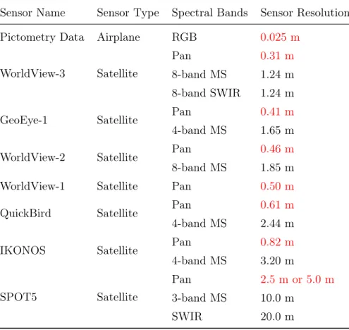
A comparison of commercial satellite and aerial images is shown in Table. 3.1. The change of spatial resolution can be seen visually in Fig.3.1.
Table 3.1: Comparison of Spatial Resolution of Commercial Satellite and Aerial Images
Sensor Name Sensor Type Spectral Bands Sensor Resolution Pictometry Data Airplane RGB 0.025 m
WorldView-3 Satellite
Pan 0.31 m
8-band MS 1.24 m 8-band SWIR 1.24 m
GeoEye-1 Satellite Pan 0.41 m
4-band MS 1.65 m
WorldView-2 Satellite Pan 0.46 m
8-band MS 1.85 m
WorldView-1 Satellite Pan 0.50 m
QuickBird Satellite Pan 0.61 m
4-band MS 2.44 m
IKONOS Satellite Pan 0.82 m
4-band MS 3.20 m
SPOT5 Satellite
Pan 2.5 m or 5.0 m
3-band MS 10.0 m
3.2
A ‘Brief ’ History of Computer Vision
Computer vision is a discipline that aims to analyze and interpret scenes of the real world [18]. Its ultimate goal is to model, duplicate and exceed the abilities of human vision sys-tem through electrical hardware and computational models [2]. Computer vision overlaps significantly with image processing and pattern recognition, and typical tasks of computer vision include object recognition, motion analysis and 3D scene reconstruction.
In 1960, for the first time, Larry Robert’s Ph.D. thesis discussed the possibility of extracting 3D geometrical information from 2D perspective views [19]. Researchers started to follow this work and studied computer vision. In 1966, Marvin Minsky at MIT assigned computer vision as an undergrad summer project. Later, much research was done in “low-level” image processing such as edge detection and segmentation.
The most widely cited article in computer vision history is the Scale Invariant Feature Transform (SIFT) paper [20]. It was introduced by David Lowe in 1999 to provide local feature descriptors [21]. SIFT was widespread in the geometric field of computer vision and it served later as the basis of the Bag of Words (BoW) model for object recognition.
In 2003, Caltech-101 as a dataset of images was created by Feifei Li. It opened the door to an era of large-scale datasets. Researchers started to run and evaluate their algorithms on these publicly available datasets. It offered researchers an objective and standard way to compare their algorithms with state-of-the-art methods.
Visual words were also introduced in 2003. It was an algorithm from text recogni-tion and has been applied to object recognirecogni-tion. Visual words are a fairly robust way to represent the content of an image and is still heavily utilized. Another factor for rise of computer vision was the widespread use of the support vector machine (SVM) as a robust, accurate and easy to use learning algorithm.
In 2005, Histogram of Oriented Gradients (HOG) was introduced to solve the problem of pedestrian detection [22]. In 2006, spatial pyramid was applied as an extension of bag-of-features image representation [23]. In 2008, the strength of the HOG was reinforced by Deformable Part Models [24]. At this stage, researchers poured a lot of effort into the design of better features.
With the development of the Internet, researchers could acquire a cheap and limitless source of images. Labeled datasets with millions of images became available. For exmaple, ImageNet consists over 15 million labeled high-resolution images in over 22000 categories [25].
Neural networks are a very old technique but they were overshadowed by SVM for a long time. However, with the significant increase of GPU computing capability, Big Data started to unlock the capabilities of neural networks. They began to rival SVM. Convolutional neural network have produced stellar results and their capabilities are illustrated in the ImageNet Large Scale Visual Recognition Challenge. The performance is now close to humans.
3.3
Computer Vision in Remote Sensing
Since the remote sensing and computer vision communities share a common goal of ex-tracting useful information from raw imagery [26], computer vision can make important contribution to the analysis of remote sensing imagery.
However, the resolution of early satellites was too coarse. Thus, image analysis tech-niques for those imagery are confined to pixel-based analysis or even sub-pixel analysis and the applications are limited to land use and land cover classification using spectral information. Then, computer vision techniques had not much importance except in low-level processing such as image filtering, contrast enhancement, edge detection and region segmentation [3].
With the emergence of imaging sensors with very high spatial resolution, the rapid development of computer vision had enormous impact on processing and interpretation of remotely sensed data. A number of application areas have evolved linking the two fields, such as road detection, building modeling and vehicle tracking. Recognition of limitations with pixel-based image approaches [8], there was a hype in applications beyond pixels [5]. A segmentation algorithm is used to divide the image into homogeneous regions which could be recognized by shape, texture and context information extraction by techniques from computer vision.
Today, more researchers are adopting computer vision methods to remote sensing and working at the forefront of combining knowledge from both fields. The gap between these two fields is getting smaller as remote sensing has benefited from great improvements in computer vision.
3.4
Deep Learning in Remote Sensing
Recently, deep learning techniques have demonstrated excellent performance on various tasks and have drawn increased attention from remote sensing community.
Convolutional neural network (CNN) was employed to classify hyperspectral data using spectral information and experimental results demonstrate that the method achieved bet-ter performance than some traditional methods, such as support vector machines (SVM) [27]. An saliency-guided unsupervised feature learning framework using deep network was proposed in [28] for scene classification. In [29], Romero et al. proposed a greedy layerwise unsupervised sparse features using CNN for pixel classification. A systematically review of the state-of-the-art deep learning-based methods in remote sensing image analysis was made by Zhang et al. in 2016 [30].
(a) Landsat 7 [10] (b) SPOT 5 [11] (c) IKONOS [12]
(d) QuickBird [13] (e) WorldView-1 [14] (f) WorldView-2 [15]
(g) GeoEye-1 [16] (h) WorldView-3 [17] (i) Pictometry Image
Debris Detection
Debris detection after natural disasters such as tornadoes, hurricanes or tsunamis, is needed for effective debris removal and allocation of limited resources. It can be performed man-ually, but such effort is labor intensive and hinders the quick response needed in large hurricane impact zones. Significant advances in aerial image acquisition have greatly pro-moted the possibilities for rapid and automated detection of debris.
In this chapter, a robust debris detection algorithm using the texture feature of debris area is proposed. Section 4.1 reviews the previous research for debris detection. Section 4.2 states the method proposed. Results are provided in section 4.3 and conclusions are drawn in section 4.4.
4.1
Previous Research
In this dissertation, debris detection means delineation of debris areas in the aerial imagery. Debris piles contain concrete, asphalt and wood material from damaged roof caused by hurricanes or tornados.
Debris detection is part of disaster assessment. In the literature, many methods have been proposed to address this problem.
Pixel-based methods have been proposed for debris detection. For example, Zoltan Szantoi et al. developed an algorithm to locate downed tree debris using Leica Airborne Digital Sensor(ADS40) data[31]. A sobel edge detection algorithm was combined with spectral information based on color filtering.
With the increase in data resolution, object based methods became a popular choice for 12
debris detection. In 2008, Fumio Yamazaki et al. used imagery acquired before and after the 2007 Off-Mid-Niigata earthquake to detect building damage [32]. Supervised object based classification was performed to extract the debris of collapsed buildings. In 2011, Takumi Fukuoka et al. conducted an analysis to estimate the distribution and the amount of tsunami debris [33]. A supervised classification was performed on the post-tsunami aerial photos. In 2011, Shunichi Koshimura et al. developed an object-based method for tsunami impact mapping using QuickBird data [34]. Ground objects are classified into six classes: vegetation, water, soil, building, road and debris. The debris was labeled with a larger standard deviation than other objects of NIR band. Thresholdσ >55.0was applied. In some literature, pixel and object based methods are compared. In 2007, Jae Sung Kim et al. implemented a hurricane damage assessment using before and after Katrina image data [35]. Landsat 7, Quickbird and IKONOS satellite imagery were first classified using both pixel and object based approaches. Change detection was then performed to compare each class before and after Katrina to identify and quantify the damaged area. In 2008, Myint et al. compared pixel based and object oriented classification approaches on identification of tornado damaged areas [36]. Accuracy assessment revealed that the ob-ject based image analysis(OBIA) approach outperforms pixel-by-pixel analysis in damage detection.
With the increase in data resolution, pixel-based analysis has been replaced by object based method. Features extracted from object level are considered for better performance. Lots of research have been done about debris mapping. However, these techniques have never been tested on very high resolution Pictometry data. The aim of our research is to develop a robust debris detection for the one-inch-resolution data.
4.2
Approach
Traditional remote sensing techniques like change detection, anomaly detection and super-vised classification were first tested. A Fast Fourier transform (FFT) based debris detection algorithm was proposed. However, these methods did not provide promising results.
Since the pixel-by-pixel analysis did not work, OBIA framework was chosen for debris detection on Pictometry one-inch-resolution data. The image is first grouped into homo-geneous objects. Texture and spatial features are extracted from each object. A debris detection algorithm using texture variance is proposed. Meanwhile, the parameter
selec-tion for segmentaselec-tion scale and kernel size is discussed. Robust assessment is performed on large scale images. The data are 8-bit values ranging from 0 to 255.
4.2.1 Data
The data used for experiments was provided by Pictometry International. The spatial resolution is around one inch. Two sets of data are provided as shown in Table4.1.
Table 4.1: Data Sets Provided by Pictometry International for Debris Detection Name of Storm Date Location Data Type
Hurricane Ike Sep, 2008 Galveston, Texas Pre and Post Moore Tornado May, 2013 Moore, Oklahoma Post
Hurricane Ike was the third-costliest hurricane ever to make landfall in the Unites States and the costliest hurricane in Texas history. The Moore tornado struck Moore, Oklahoma, and adjacent areas on May 20, 2013, killing 23 people and injuring 377 others.
The Pictometry Online Interface (POL) provides web based access to Pictometry im-agery. Pictometry images every location multiple times, with different views. In this study, only the Ortho images are used. Twenty large scale images of each data set are tested in the experiment. Fig. 4.1 shows samples of before-and-after aerial imagery collected by Pictometry.
4.2.2 Statistical and frequency analysis of debris area Statistical and spatial frequency analysis on the debris area is performed.
As shown in Fig. 4.2, before-and-after hurricane Ike images are pixel to pixel regis-tered. Mean radiance and standard deviation of before-and-after hurricane Ike images are calculated.
Table 4.2 shows that the mean radiance value is increased after Ike. The standard deviation is also increased. The value is band averaged. The average radiance values are increased because the main materials of debris are concrete and wood with relative higher radiance values than other materials. The standard deviation is increased because of the complexity of debris area. Standard deviation can be used for debris detection as proposed
(a) Pre-Ike data (b) Post-Ike data
Figure 4.1: Before-and-After hurricane Ike images
by Shunichi Koshimura et al. [34]. They used the threshold of standard deviationσ >55.0
to detect the debris area.
Table 4.2: Mean and Standard Deviation (Std) Values of Before-and-After Hurricane Ike Subimages.
Pre-Ike data Post-Ike data
Mean 154 176
Std 45 59
Frequency analysis of before-and-after hurricane Ike images are shown in Fig.4.3. The Fourier spectrum of the no-debris area is relatively structured compared to the spectrum of the debris area, especially in the high frequency domain. It can be seen more clearly through the Fourier spectrum of the images as shown in Fig.4.4.
(a) Pre-Ike data (b) Post-Ike data
Figure 4.2: Before-and-After hurricane Ike images
(a) FFT of no debris area (b) FFT of debris area
Figure 4.3: Fourier spectrum of no-debris and debris area
4.2.3 FFT based debris detection algorithm
A detection method is proposed based on the frequency analysis of debris area. The method is established on the fact that, for a no debris area with directional or periodic texture, the magnitudes of its Fourier spectrum will concentrate on a certain direction or several directions. For debris area with random texture spreads out over all directions, i.e., for random textures, the distributions of the responses of spectra are not restricted to certain directions.
First, a Fourier transform is applied to the local region extracted by a w×w sliding window. For a square image of sizew×w, the two dimensional Discrete Fourier Transform (DFT) is given by:
(a) No-Debris Area (b) Debris area
(c) Fourier spectrum of no-debris area (d) Fourier spectrum of debris area
Figure 4.4: Fourier spectrum of no-debris and debris area
F(k, l) = w−1 X i=0 w−1 X j=0 f(i, j)e−i2π(kiw+ lj w) (4.1)
wheref(a, b)is the image in the spatial domain and exponential term is the basis function corresponding to each point F(k, l) in the Fourier space. Then, each spectrum window is smoothed by convolving with a 2D Gaussian kernel. Then, as shown in Fig. 4.5, the spectrum “pie” is divided into 8 pieces and the summation of pixel value in each piece is calculated. The standard deviation of these summations is calculated and saved for the center pixel of the sliding window. According to the frequency analysis, the standard deviation should be lower for debris area. A threshold can be applied to extract the debris. The results are provided in Section 4.3.
4.2.4 Object based debris detection algorithm
Object based imagery analysis (OBIA) works on the object level instead of the pixel level. In contrast to traditional pixel-based methods that classify individual pixels directly, object-based classification first groups pixels into homogeneous objects. The feature of each segment can be extracted and used for the following processing.
Figure 4.5: Fourier spectrum analysis
There are several software packages available to perform OBIA, such as eCognition, Feature Analyst and Feature Extraction. Our algorithm is fulfilled using the Feature Extraction module in ENVI software from ITT Visual Information Solution.
As shown in Fig. 4.6, the algorithm can be divided into three steps: interactive seg-mentation, feature extraction and thresholding.
Figure 4.6: Framework of OBIA debris detection
The first step is segmentation with a proper scale. If the segment is too small, it can not capture the texture feature of debris. If the object is too large, it can not separate the debris from others.
The segmentation in ENVI Feature Extraction is controlled by two parameters: scale level and merge level. ENVI uses two numbers between 0 to 100 to represent the degree of segmentation and mergence. The scale level controls relative segment size. The segment size should adjusted to be able to represent the minimum-sized debris. The merge level controls the degree of merging contiguous segments into larger objects. A scale level of 25 followed by merge level of 99.7 is selected by trail and error.
The segmentation inside ENVI Feature Extraction includes two steps: a gradient map is first computed using a sobel edge detector and watershed algorithm is then applied on
the gradient map to get the segmentation result.
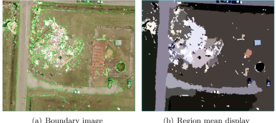
Fig. 4.7(a)shows that values of 25 for Scale level and 99.7 for Merge Level effectively delineate the boundaries of debris area. Fig. 4.7(b) is the region mean display of the segmentation result.
(a) Boundary image (b) Region mean display
Figure 4.7: Segmentation result with Scale Level 25 and Merge Level 99.7
After the segmentation, the image is separated into individual objects as shown in Fig.4.7(b), then spectral, texture and spatial features of each object can be computed and used for the following classification.
The most obvious difference between debris and no-debris area is texture pattern. The texture pattern of debris is random while others is relative uniform. Thus, texture feature should be extracted for debris detection. Four texture attributes are available in Feature Extraction: texture range, texture mean, texture variance and texture entropy.
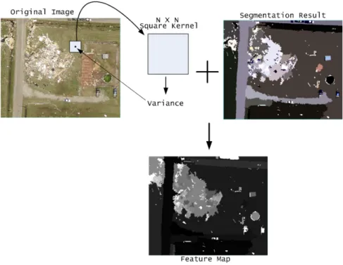
As shown in Fig.4.8, the texture features are calculated in the following steps. Ak×k
square kernel is applied on the image. Range, mean, variance and entropy are calculated for pixels inside the kernel window. Result is referenced to the center pixel. Average the values inside each segment to create the feature map.
The texture range attribute (kernel size 3) images are shown in Fig.4.9. A higher gray level means higher texture range value. From Fig.4.9, we can easily identify debris with high texture range value. Meanwhile, we find that in the very-high-resolution(VHR) aerial image, the texture feature of cars is similar to debris object. The aerial image provided by Pictometry is a 3 band image. The attribute image of each band is compared. There is no obvious difference among the R, G and B bands.
Figure 4.8: Texture feature calculation
Texture mean was rejected as a feature because it does not work for asphalt debris.The texture mean attribute image is shown in Fig.4.10. Texture entropy is also rejected because it can not distinguish debris and no-debris area. This attribute image is shown in Fig.4.11. Texture variance attribute images are shown in Fig. 4.12. Now, we need to make a choice between texture range and variance.
Another parameter, kernel size, is considered. Attribute images of texture range with different kernel sizes are shown in Fig.4.13. With the increase of kernel size, the texture
(a) Original image (b) R band (c) G band (d) B band
(a) Original image (b) R band (c) G band (d) B band
Figure 4.10: Attribute image of texture mean
Figure 4.11: Attribute image of texture entropy (R band)
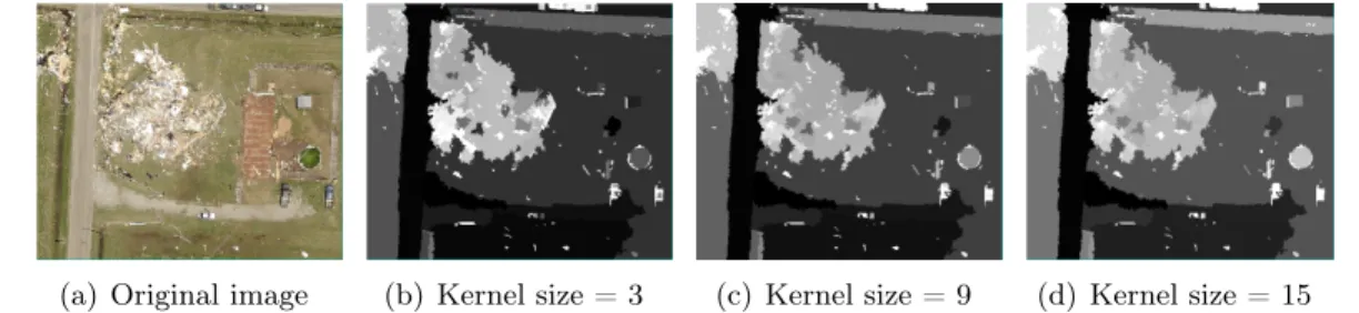
range of the undamaged roof would increase. It may result in false alarm.
Attribute images of texture variance with different kernel sizes are shown in Figs.4.14. The obvious difference between Figs. 4.13 and Figs. 4.14 is that the attribute value of land and road would not change when kernel size is increased. Thus, texture variance is selected. Kernel size is set to 15, to increase the probability of detection of large concrete debris. A threshold of 1800 for texture variance is set to obtain the final result. More
(a) Original image (b) R band (c) G band (d) B band
(a) Original image (b) Kernel size = 3 (c) Kernel size = 9 (d) Kernel size = 15
Figure 4.13: Attribute images of texture range with different kernel sizes
results are provided in Chapter 5.
(a) Original image (b) Kernel size = 3 (c) Kernel size = 9 (d) Kernel size = 15
4.3
Results
Two methods are proposed for debris detection: Fast Fourier transform (FFT) based method and object based image analysis (OBIA) method as described in section 4.2.
4.3.1 FFT based debris detection algorithm
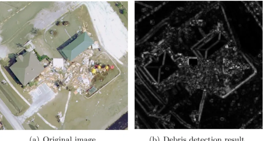
The result of the FFT based debris detection algorithm is shown in Figs.4.15. According to the frequency analysis, the standard deviation of summations of pixel values in each spectrum piece should be lower for debris area. A threshold can be used to extract the debris.
(a) Original image (b) Debris detection result
Figure 4.15: FFT based debris detection Result
However, in the result, uniform areas show lower standard deviation than debris areas. Thus, this method can not be used for debris detection.
4.3.2 OBIA debris detection algorithm
The OBIA debris detection framework is shown in Fig.4.16. The detection algorithm using texture variance provides us a general location of debris.
Texture variance with kernel size 15 is extracted from each segment. The segment scale is set to 25 and merge scale is 99.7. The debris detection results just based on the texture variance are shown in Fig. 4.17. The detection result is promising with threshold 1800.
Most of the debris is detected, even small areas. However, the car and the edge of a pool are misclassified as debris.
More data are involved in the robust assessment and the results are shown in Figs.4.18
-4.20. We have compared results performed on all bands and found that the blue band gives the best results.
In Fig.4.18, the algorithm detects the uprooted trees around the building. The debris pile at the lower right corner consisting of concrete and wood is also detected. The trunks of uprooted trees at the left part of the image are located. Tree crown would be detected if red and green band are used with threshold of texture variance 1300. The edge of the road is misclassified as debris. Compared to data 1, most of the data 2 is no-debris area. In the result shown in Figs.4.19, most part of the image 2 is labeled as no-debris area. It detected the debris at the upper left corner of the image. Cars are misclassified as debris because of their complex texture pattern. Most debris at the right part of data 3 are detected as shown in Figs.4.20. However, the algorithm fails to find the the debris pile in the forest at the left part of image. In general, the results are acceptable on large scale data.
(a) Original image (b) Detection result
(a) Original image
(b) Debris detection result on blue band
(a) Original image
(b) Debris detection result on blue band
(a) Original image
(b) Debris detection result on blue band
4.4
Conclusion
Debris detection is needed for effective debris removal and allocation of limited resource. The frequency analysis of no-debris and debris areas is performed and it shows that the frequency spectrum of non-debris area is relatively structured compared to debris area. Thus, a Fast Fourier transform (FFT) based debris detection algorithm is proposed. Al-though the method did not provide promising results, it sets a direction for future research. A more effective way to use the frequency feature of debris area could be investigated. An-other debris detection algorithm under object based image analysis(OBIA) framework was proposed. The algorithm can be divided into three steps: interactive segmentation, feature extraction and thresholding. The interactive segmentation is performed using ENVI Fea-ture Extraction module. TexFea-ture variance inside each segment is extracted to create the feature map. Thresholding is applied to get the debris detection result. According to the visual inspection, the performance is promising and robust on large scale data. Compared with traditional pixel-based methods which can require pre-and post-disaster imagery, the proposed method utilizes the texture feature more efficiently at the object level. Compared with traditional disaster assessment methods, only post-disaster imagery is needed to fulfill the debris detection with methods proposed here providing robust results.
Building Detection
Robust building detection is an important part of high resolution aerial imagery under-standing [6]. Building detection also serves as pre-processing for building modeling and roof condition assessment applications.
In this chapter, a 3D scene classification algorithm for building detection using point clouds derived from multi-view imagery is proposed. Section 5.1 reviews the previous research for building detection. Section 5.2 states the method proposed. Results are provided in section 5.3 and conclusions are drawn in section 5.4.
5.1
Previous Research
Buildings are one of most important man-made objects in aerial images. Many studies have explored robust building detection. In this dissertation, building detection means labeling the building objects in point clouds derived from multi-view imagery. Plenty of approaches have been proposed and can be grouped into two basic categories [37].
The first group use purely mathematical models and geometric reasoning techniques [37]. In 2001, G.Sithole et al. assumed that the natural terrain surface does not have slopes above certain threshold. Based on this assumption, a slope adaptive filter was proposed to remove non-ground objects[38]. In 2007, Schnabel et al. presented an algorithm to detect basic shapes in point clouds based on RANSAC [39]. The algorithm is fast while still maintaining accuracy. In 2009, Sirmacek et al. used scale invariant feature transform (SIFT) and graph theoretical tools to extract separate buildings in the urban area [40]. In 2013, Sun et al. used a graph cut based method to segment vegetative areas using Lidar
data [41]. A hierarchical Euclidean clustering was used to extract the ground terrain and building rooftop patches. Running time of these approaches is fast. However, they may be not robust for complex scenes [37]..
Another category uses machine learning theory [37]. 3D structure features are extracted for classification. Promising result can be provided even in complex scenes. In 2005, Muller et al. performed a seeded region growing algorithm [6]. Photometric and geometric features were extracted from each segment. Classification was performed on the feature vector to get the building class. In 2006, Pu et al. divided the terrestrial laser data into individual segments using the planar surface growing algorithms [42]. Properties are computed for each segment and a rule based recognition performed. In 2008, Biosca et al. presented an unsupervised robust clustering approach for terrestrial laser data based on fuzzy methods [43]. The drawback of these methods is that the feature extraction processing is time consuming [37].
For this study, the data we use are point clouds derived from multi-view imagery pro-vided by Pictometry International. The techniques of point cloud generation in Pictometry are still under development. The quality of data is far from perfect. Lots of existing meth-ods may not work for our data. We need to investigate methmeth-ods specific for the Pictometry point cloud data. For the future, spectra, texture, shape or morphological features [44] from one-inch-resolution imagery should also be considered to improve the accuracy.
5.2
Approach
There are many segmentation methods available for 3D scene segmentation. However, at this point, the quality of point clouds provided by Pictometry International is limited. The goal of our research is to investigate methods that will work with limited quality point clouds.
5.2.1 Data
Point clouds derived from multi-view imagery were provided by Pictometry International. Sample data are shown in Fig. 5.1 and were derived from image shown in Fig. 5.2. A detail is shown in Fig.5.3. We can see that two small rooftops are noisy with some outliers located near the boundary of the rooftop. Fig.5.4shows a large scale scene of point clouds.
Figure 5.1: Point cloud provided by Pictometry International
Figure 5.2: Image provided by Pictometry International
5.2.2 Simple algorithm exploration
We started the project with a simple scene as shown in Fig. 5.1. The objective was to divide the data into tree categories: roofs, trees and ground.
The point cloud generation technique now is still under development and results in sparse outliers. Thus, pre-processing is needed to remove these outliers.
Statistical analysis on each point is performed. For each point, the mean distance from it to all itsknearest neighbors is computed. Assuming the distribution of all points’ mean distances is Gaussian, those mean distances outside one standard deviation are labeled as outliers and rejected. The before and after outlier removal data are shown in Figs. 5.5. After the outlier removal, the point cloud is relatively clear.The canopy is not integrated compared with the data before outlier removal. Man-made objects are our main interest, thus the result is acceptable.
Figure 5.3: Detail of point cloud
Figure 5.4: Large scale scene of point cloud
(RANSAC)[45] algorithm is used to fit all the points that support a plane model in the selected scene. The result of the RANSAC algorithm is shown in Fig. 5.6. Ground and large roofs in the simple scene are extracted. We can label them based on their average elevation. First, the average elevation of the entire scene is calculated. Then, the average heights of plane 1 and plane 2 are calculated. Assuming the elevation of roof is higher than the average height of the scene while the height of ground is lower than the average, we can label them as roof or ground. However, the small rooftops can not be extracted through RANSAC plane model segmentation since they are not flat enough to fit the plane model. The remaining areas after plane model segmentation are shown in Fig.5.7. Three small roofs and four tree canopies are left. Also, we can see some noisy parts which belong to
the ground. These noisy parts can be removed through post-processing.
Now, the mission is to distinguish small roofs from trees. The first step is still seg-mentation. Different objects in the leftover scene are spatially separated, therefore it is reasonable to apply Euclidean clustering for segmentation.
After the segmentation, the next step is to extract features from individual clusters and label them based on the extracted features. A structure feature, the average difference of normals (DoN) [46] is selected. For each point, normals with two different radius are calculated and then the difference of these two normals is computed. The average DoN of a tree cluster should be higher than that of a relative flat rooftop. A threshold is set to distinguish trees and roofs. The result of DoN based classification is shown in Fig.5.8.
5.2.3 Robust building detection using computer vision technique A robust building detection using computer vision algorithm is proposed.
As shown in Fig. 5.9, after the outlier removal and Euclidean cluster, the input point cloud is segmented into individual point clusters. The main ground can be easily identified based on the number of points it contains.
Four kinds of features are extracted from individual point clusters as shown in Fig.5.10. For each point cluster, the number and density of point cluster are computed. The height, area and also average RGB value are calculated. The curvature and DoNs are extracted as normal related features to describe the structure of point clusters. Among these features, the radius-search-based normal calculation takes most of time. To speed up the calculation, point clusters are downsampled and multi-threaded computation is applied.
With point clusters and its feature vectors, the next step is SVM classification as shown in Fig. 5.11. These manually labeled clusters are automatically divided into 3 folders. Folder 1 and 2 are used to train the SVM classifier with radius basis function (RBF) kernel. V-fold cross validation and grid search is used to find the best parameter pair for RBF kernel. Then, folder 3 is used to test the performance of trained classifier. Results are provided in Section 5.3.
(a) Point cloud before outlier removal
(b) Point cloud after outlier removal
(a) Plane 1
(b) Plane 2
Figure 5.6: Plane model segmentation result
(a) Plane 1 (b) Plane 2
Figure 5.8: DoN classification result
Figure 5.10: Feature extraction
5.3
Results
The results of the simple algorithm and the machine learning based methods for building detection are provided and discussed in the following sections.
5.3.1 Simple algorithm exploration
The framework of proposed simple algorithm for point cloud segmentation is shown in Fig.5.12.
The result of the simple algorithm is shown in Figs. 5.13. The result is perfect for the selected scene. However, this algorithm is not robust on large scale scenes like Fig. 5.4.
The first problem is that the classical RANSAC algorithm can not detect the individual plane roofs in large scale scene where the plane roofs are very small part of the entire scene. Another problem is that RANSAC would not give us the main ground for some data shown in Fig. 5.14(a). The main ground of this data is not flat enough. Even with a loose limitation, RANSAC would output a result shown in Fig.5.14(b) which is clearly not the ground.
In summary, the proposed unsupervised algorithm works perfect on the selected scene. However, it is not robust enough for large scale data.
5.3.2 Robust building detection using machine learning technique The experiment is performed on the large scale scene of point cloud shown in Fig. 5.4. The accuracy of trained Support Vector Machine (SVM) classifier is 89% with 7% false detections. The result is acceptable. Mistakes happen when the trees and rooftops are spatially connected. The Euclidean clustering can not separate them and this case results in a mixed cluster.
(a) Ground
(b) Roof
(c) Tree
Figure 5.13: Final result of our simple algorithm
(a) Data
(b) Output of RANSAC
5.4
Conclusion
Building detection is an important part of high resolution aerial imagery understanding and it also serves as pre-processing for other applications. A building detection algorithm using 3D point cloud is proposed in this thesis. Point clouds are first segmented into individual point clusters using Euclidean clustering. Spectral and 3D structure features are extracted to represent each cluster. The extracted feature vectors are used to train the support vector machine (SVM) classifier. The accuracy of the proposed algorithm is89%
Roof Condition Assessment
The inspection of roof condition is an important step of damage claim processing in the insurance industry. Automated roof condition assessment methods from remotely sensed images are proposed in this Chapter. In section 6.1, previous research is reviewed. In section6.2, texture classification and bag-of-words model are first performed to assess the roof condition using features covering the whole rooftop. Then, considering the complexity of residential rooftop, a more sophisticated method is proposed to divide the task into two stages: 1) roof segmentation (section 6.3), followed by 2) segments classification (section
6.4).
6.1
Previous Research
In this dissertation, roof condition assessment is defined as grading the roof condition based on the area of missing shingles or cosmetic damage on the roof using very-high-resolution(VHR) imagery. Very little research has been published specifically on roof con-dition assessment. There is some research for roof concon-dition using spectral information. In 2016, Samsudin et al. proposed spectral indices to generate degradation status maps of concrete and metal roofing materials using multispectral imagery [47].
In the literature, the closest field we found is building damage assessment. The al-gorithms on building damage assessment are divided into two categories: methods using both pre- and post-event data or only post-event data. The methods working with pre- and post-event data provide more promising results. However, pre-event data are not always available.
As shown in Fig.6.1, building damage can be classified into five damage grades: slight damage, moderate damage, heavy damage, very heavy damage and destruction in the European Macroseismic Scale 1998 (EMS98) [1].
(a) Grade 1: Negligible to slight damage
(b) Grade 2: Moderate damage
(c) Grade 3: Substantial to heavy damage
(d) Grade 4: Very heavy damage
(e) Grade 5: Destruction
Figure 6.1: Classification of damage to masonry buildings [1]
In 2009, Sirmacek et al. extracted building rooftop based on color invariants and shadow region using grayscale histogram. A damage measure derived from rooftop and shadow was proposed [48].
In 2010, Brunner et al. proposed a damage detection algorithm based on the similarity between predicted and actual synthetic aperture radar (SAR) data [49]. 3D parameters are derived from pre-event optical imagery and used to predict signature of the building without damage in the post-event SAR scene.
In 2011, a supervised classification algorithm was proposed by Gerke et al. to divide the scene into facades, intact roofs, destroyed roofs and vegetation using oblique Pictometry data [50]. 22 features were used. The role of features in classification was discussed. Damage score was derived from classification results from different viewing direction. EMS 98 standard was adopted. The accuracy of 70 percent for scene classification and 63 percent for building damage assessment were achieved. The benefit of using oblique Pictometry data is that the condition of facades can be assessed.
In 2011, Bignami et al. studied the sensitivity of objects textural feature with respect to damage levels using pre and post-event QuickBird data. Four texture features: contrast,
dissimilarity, entropy and homogeneity were extracted from the building object [51] and tested regarding to different damage scale in EMS98.
According to Dong et al.’s review [52], heavy damage grades such as grad 5 in EMS98 are detectable. The challenge is identification of lower damage grades, even with a sub-meter resolution data [52]. In other words, most literature on damage assessment is about damage detection. Labeling the exact damage grade of a building is still a barrier. Compared to building damage assessment, roof condition assessment is a more sophisticated task because the emphasis of roof condition assessment is placed on grading lower damage grades.
In this dissertation, we aim to assess the roof condition using features covered the whole roof at first. Then, a novel method containing roof segmentation and segments recognition is proposed to provide a more subtle assessment.
6.2
Preliminary roof condition assessment
In this section, the preliminary roof condition assessment using feature extracted from the entire roof sample is performed. Texture classification and bag-of-words (BoW) model are applied.
6.2.1 Approach
6.2.1.1 Data
The data for this research consisted of one inch ground resolution color airborne imagery collected by Pictometry International. For this study, we manually extracted the roof sample images as shown in Fig. 6.2. Rooftops of interest were cut out from the imagery and a rotation was followed by additional cropping to obtain the final experimental sample images.
110 intact roofs and 164 damaged roofs were manually extracted from 469 high reso-lution images provided by Pictometry. Typical roof sample images are shown in Fig. 6.3. Cosmetic damage and missing shingles are the most obvious features of damaged roofs.
A challenge with these data is the high within-class diversity in the intact roofs and damaged roofs as shown in Figs. 6.4- 6.5. Features extracted from the entire rooftop may not be sufficient for automated condition assessment.
Figure 6.2: Manual data extraction
6.2.1.2 Texture classification
Texture features: Gray-Level Co-occurrence Matrix(GLCM), Local binary patterns(LBP) and Gabor filter have achieved great success in texture classification. Since the resolu-tion of Pictometry data is around one inch, texture informaresolu-tion is a reasonable choice to distinguish intact roofs from damaged ones.
The framework is shown in Fig. 6.6. We manually extract the experiment sample images and label them. As shown in Fig. 6.7, texture features are extracted. Statistical features: variance, standard deviation, skewness, kurtoisis, uniformity and entropy of each roof sample image are computed. Dissimilarity, correlation, homogeneity, contrast, ASM and energy are extracted from GLCM computation. LBP histogram is added to the feature vector. Meanwhile, mean and variance of Gabor filtered image are added. In summary, for each roof sample image, 72 features are calculated.
(a) Intact roof (b) Damaged roof
(c) Damaged roof
Figure 6.3: Pictometry rooftop sample images
useful features. A SVM linear kernel is trained on the initial set of features and weights (coefficients) are assigned to each one of them. Then, the features with smallest absolute weight are removed. The procedures are recursively repeated. The processing of RFE is shown in Fig. 6.8. Finally, 16 features which give the best classification accuracy are selected. The 16 selected features are used for the following SVM classification.
Feature vectors with labels are randomly divided into 2 folders. Folder 1 are used to train the SVM classifier with Polynomial kernel. Folder 2 are used to test the trained SVM classifier. Results are provided in Section 6.2.2.
6.2.1.3 Bag of Words model
The BoW model is a classical computer vision technique used for content based image retrieval. Here, BoW is used for preliminary roof condition assessment. The basic flow for BoW is:
• Use Dense SIFT to collect lots of features from training images. • Use K-means to cluster those features into a visual vocabulary.
(a) Shadow (b) Dust (c) Tree (d) Window
Figure 6.4: Intact rooftop sample images with high within-class diversity
(a) Sample 1 (b) Sample 2
Figure 6.5: Damaged rooftop sample images with tiny missing shingles
• For each of training images build a histogram of word frequency (assigning each feature found in the training image to the nearest world in the vocabulary).
• Feed these histogram to train an SVM classifier.
• Build a histogram for each of test images and classify them with the trained SVM. The framework of BoW is shown in Fig. 6.9. Results are provided in Section 6.2.2.
Figure 6.6: Traditional texture features based classification framework
Figure 6.8: Recursive feature elimination
6.2.2 Results
The objective of preliminary roof condition assessment is to divide the roof images into intact roofs and damaged ones. The results of two proposed methods are presented and discussed bellow.
6.2.2.1 Results of texture classification
Experiments are performed on the 110 intact roofs and 164 damaged roofs which were manually extracted from 469 high resolution images provided by Pictometry International. The result of texture classification is shown Table 6.1. The definitions of precision, recall and F1 are: P recision= tp+tpf p,Recall= tp+tpf n and F1 = 2· P recision·Recall
P recision+Recall where
tis for true,f is for false, pis for positive and nis for negative.
Table 6.1: Results of Texture Classification
Class Precision Recall F1-Score
Intact roof 0.83 0.55 0.66 Damaged roof 0.75 0.93 0.83
16 selected features derived from Recursive feature elimination (RFE) are used. For the trained SVM classifier, a polynomial kernel are selected. Penalty parameterC of error term is set to 10. The degree of polynomial is set to 5. From the result, we can see that the high within-class diversity in intact roofs class leads to relatively low classification performance.
If all the features are used, the result is shown Table 6.2. For the trained SVM, polynomial kernel is used. C is 10 and degree is 4. There are no false positives in this result. It can serve as a pre-processing step to eliminate part of intact roofs. The recall is low due to the complexity of our selected experiment sample images.
6.2.2.2 Results of bag of words (BoW) based classification
The best result of BoW is shown in Table 6.3. After RFE, only 2 features are selected. The linear kernel is used.
Table 6.2: Result of Texture Classification without Feature Selection
Class Precision Recall F1-Score
Intact roof 1.00 0.15 0.25 Damaged roof 0.64 1.00 0.78
Table 6.3: Result of BoW
Class Precision Recall F1-Score
Intact roof 0.77 0.73 0.75 Damaged roof 0.82 0.85 0.84
According to the F1-Score, it is the best result we achieved for preliminary roof condition assessment. Consider the complexity of residential roof, this result is not that bad. However, BoW method suffers random problem caused by K-means.