A Dynamic Model of Endogenous Exchange Rate Pass-Through

A Dynamic Model of Endogenous Exchange Rate

Pass-Through

Tokhir Mirzoev

First draft: November 14, 2003

This version: May 31, 2004

Abstract

This paper examines a two-country new open economy macroeconomics model with price stick-iness `ala Taylor, where exporters’ choice of invoicing currency is endogenous. Besides generating incomplete pass-through, the model yields four main results. First, firms’ invoicing strategy is generally time-varying. Second, instant pass-through into import prices is greater than into export prices when depreciations are caused by domestic monetary expansions. Thirdly, average pass-through is asymmetric in times of persistent depreciations and appreciations. It is higher under depreciations when the destination market is more competitive. Finally, cross-country differences in money supply variability produce an origin-based asymmetry: different average pass-through rates into import and export prices.

JEL Classification: F41, F31

Keywords: exchange rate pass-through, new open economy macroeconomics

∗_{Department of Economics, The Ohio State University, 1945 North High Street, Columbus,}

OH 43210, Tel: (614) 292-6701, Email: [email protected]. I’m thankful to Bill Dupor, Mario Miranda and especially to Paul Evans for valuable advice and useful discussions and to Raphael Solomon for useful comments. I have also benefited from comments of the seminar participants at Ohio State University, the Fourth Annual Missouri Economics Conference and the annual meetings of the CEA and WEA. All remaining errors are mine. MATLABr _{codes corresponding to this}

1

Introduction

The new open economy macroeconomics (NOEM) literature has recently attracted great attention of researchers as a convenient optimization-based framework for an-alyzing old issues in international macroeconomics. One of the central questions in the NOEM is the elasticity of import prices with respect to exchange rate shocks, often called the ”exchange rate pass-through”. The issue of pass-through is impor-tant for these models because welfare implications of monetary policy shocks and the optimal monetary policy itself have been shown to depend critically on pass-through elasticity.1

An emerging consensus in empirical research is that short-run pass-through of exchange rate shocks into import and export prices is neither 0 nor 1. Campa and Goldberg (2002) find average pass-through for 25 OECD countries to be roughly 57%. Campa and Gonz´alez (2002) and Faruqee (2004) estimate pass-through elas-ticities for the Euro area. Most of their estimates lie strictly between 0 and 100%. Olivei (2002) and Coughlin and Pollard (2000) find incomplete, but positive pass-through into U.S. import prices. Schenk (2003) estimates pass-pass-through elasticity for Canadian import prices to be close to 41% in the short-run. Kenny and McGetti-gan (1996) report partial pass-through into Irish import prices. Many other similar estimates exist2_.

Moreover, some evidence points to a number of asymmetries in pass-through. First, Dwyer et. al. (1993) report asymmetric pass-through elasticities for Aus-tralian import and export prices between 1974 and 1992. Second, in a study of dis-aggregated US import prices between 1982 and 1990, Coughlin and Pollard (2000, 2003) find that in times of depreciations higher pass-through is more likely across industries. Wickermasinghe and Silvapulle (2003) also find statistically significant asymmetric response of Japanese manufactured import prices, although their re-sponse seems to be higher in times of appreciations. Finally, in their 2003 paper

1_{See, respectively, Obstfeld and Rogoff (1995) vs. Betts and Devereux (2000), and Engel (2002).} 2_{E.g. Krugman (1987), Knetter (1989, 1993), Dwyer et. al. (1993), Coughlin and Pollard}

Coughlin and Pollard report a positive correlation between the rate of pass-through into U.S. import prices and the size of the exchange rate depreciation. Theoretical literature is mostly devoted to the size of pass-through and seems to have overlooked the issue of its asymmetry.

Limited aggregate pass-through can occur for many reasons. Two recent papers, Bachetta and van Wincoop (2002) and Devereux, Engel and Storgaard (2002),

ex-amine optimal choice of invoicing currency in the context of NOEM 3_{. Both papers}

provide a useful analysis of firms’ decisions. Their models assume one period in ad-vance pricing, so that all prices are assumed predetermined in every period. Thus, when firms are identical the only equilibrium is a corner solution: pass-through is either 0 or 1. Limited pass-through can only be generated by intratemporal hetero-geneity of invoicing decisions. However, the latter often implies multiple equilibria, which complicates a dynamic analysis.

In this paper we study another scenario. We assume endogenous invoicing and symmetric firms, but with staggered price adjustment. The model generates a pass-through that is always incomplete due to firms’ intertemporal heterogeneity and a unique equilibrium in this setting is easier to find. Another advantage is that the model is more dynamic and sheds some light on potential causes of asymmetries in pass-through.

We point out several key model ingredients. First is Taylor-type two-period price stickiness. The model assumes two cohorts of firms in every sector, each up-dating prices in turn and at different dates. Each date’s new prices are valid during both the current and the next period. When re-optimizing, exporting firms also

choose the currency in which to specify their prices 4_{. The size of every period’s}

aggregate pass-through thus depends on both past invoicing decisions of the firms whose prices don’t change as well as the size of price adjustment by re-optimizing firms. This also ensures a time-varying pass-through rate. Although in every period

3_{Menon (1995) provides a helpful review of earlier theoretical developments.}

4_{One could think of this as being the decision of whether to index the price to the exchange rate}

or not. Another example would be an international catalogue seller. Before printing the catalogue, the seller could choose which currency to specify the prices in.

the pass-through into the unadjusted prices is either zero or one, pass-through into aggregate import price index is always positive and incomplete. We emphasize ag-gregate pass-through as opposed to pass-through into individual prices, because the available evidence is mostly based on industry-level data and tells us little about behavior of individual firms.

Another feature of Taylor pricing is that firms maximize the sum of current and future expected profits. This raises the importance of conditional means of variables. Our main finding is that optimal invoicing strategy is generally different depending on whether the currency is under- or over-valued relative to the long-run equilib-rium. This makes possible asymmetric pass-through rates in times of persistent depreciation or appreciation.

Finally, we assume incomplete markets, so that unexpected shocks create devia-tions from the interest parity and risk sharing condidevia-tions. As a result, one country’s monetary expansion will have asymmetric effects on consumptions and real wages across countries. Therefore, pass-through into import prices depends critically on the origin of the shock. This gives a simple explanation of the second type of asym-metry. In our benchmark model, domestic monetary expansions affect import prices by more than they affect the foreign currency value of export prices. As a conse-quence, in the long-run a country with higher money supply variability experiences

higher pass-through into its import prices.5

To summarize, the setting we consider predicts: 1) incomplete and time-varying short-run exchange rate pass-through; 2) asymmetric average pass-through in times of persistent depreciation or appreciation; and 3) a possibility of asymmetric average

pass-through into import and export prices. 6

The rest of the paper is organized as follows. Section 2 describes the model and

5_{This result is similar to the finding in Devereux et. al. (2002), although their motivation is}

somewhat different.

6_{A caveat should be made before interpreting our results. In this paper we do not attempt}

to match the data quantitatively. A detailed ”moment-matching” exercise would require a more elaborate model (e.g. with lengthier price stickiness, distribution costs, variable markups, etc.). Instead, we concentrate on the most basic NOEM model to show that endogeneity of invoicing deci-sions along with staggered time-dependent price adjustment produces results that are qualitatively similar to those found in the data.

equilibrium conditions. In section 3 we briefly describe how the model can be solved using the collocation method. The remaining sections discuss our findings and the intuition behind them.

2

The Model

Most features of our model are standard in the NOEM literature 7_{. The world is}

assumed to have two countries, Home and Foreign. Total population is spread over

a unit interval with a fraction n living at Home. Firms in both economies are of

two types - firms producing and selling domestically (nontraded goods firms) and exporters producing in the domestic economy but selling abroad. The mass of each type of firms is normalized to equal that of consumers, and each firm produces a differentiated product, acting as a constrained monopolist.

2.1

Consumers, Asset Markets and the Government

Consumer goods are collected into baskets `a la Dixit and Stiglitz (1977). Home

country agents purchase the home goods basketCHtfrom domestic firms and foreign

goods basket CF t from foreign exporters. These aggregates are given by:

CHt = · ¡₁ n ¢1 λRn 0 CHt(j) λ−1 λ dj ¸ λ λ−1 ; CF t = · ¡ ₁ 1−n ¢1 λR1 n CF t(j) λ−1 λ dj ¸ λ λ−1 . (1)

Home consumer’s aggregate consumption basket Ct combines the two country

goods baskets in a CES fashion:

Ct = ( nω1C ω−1 ω Ht + (1−n) 1 ωC ω−1 ω F t ) ω ω−1 . (2)

Each country has its own currency. For simplicity we will call the Home currency

dollars, and Foreign currency euros. Hereafter, variables expressed in euros are

marked with an asterisk. Foreign country variables also have a superscript F, and

an asterisk if expressed in euros. In addition, variables pertaining to exporters will

have a superscript e.

Price indices associated with each consumption aggregate are defined as the minimum nominal cost of purchasing one unit of the relevant basket. They are given by: PH t = · 1 n R_n 0 PtH(j)1−λdj ¸ 1 1−λ ; PeF t = · 1 1−n R₁ nPteF(j)1−λdj ¸ 1 1−λ ; (3) Pt = ( nP_tH(1−ω)+ (1−n)P_teF(1−ω) ) 1 1−ω . (4)

The baskets/indexes imply the following demands for individual goods and coun-try baskets: CHt(j) = 1 n · PH t (j) PH t ¸−λ CHt; and CHt =n · PH t Pt ¸−ω Ct (5) CF t(j) = 1 1−n · PF t (j) PF t ¸−λ CF t; and CF t = (1−n) · PF t P ¸−ω Ct (6)

All consumers are identical. They supply labor, eat, and hold equal ownership in all domestic firms (including exporters). In addition, agents hold money balances, from which they derive utility, and bonds.

Asset markets are incomplete. There are two types of nominal non-state-contingent

bonds in this economy: a Home bond (BH

t ) denominated in the Home currency and

sold only domestically and a Foreign bond (Bt) denominated in the foreign currency

it and i∗t, respectively, at date t+ 1. The assumed structure of asset markets allows

ex-post deviations from the uncovered interest parity and risk sharing conditions. Firms’ profits are distributed as dividends, which consumers take as given. Home

consumers enter each period with the previous period’s bonds (BH

t−1) and money

balances (Mt−1), and choose consumptionCt,new bond and money holding BtH,Bt,

Mt, and labor supply Lt in order to maximize expected life-time utility:

maxE0 ∞ X t=0 βt à C1−σ t 1−σ + χ 1−ε µ Mt Pt ¶_1−ε − κ ψL ψ t ! (7)

Subject to a budget constraint:

CtPt ≤ −BtH −etBt+ (1 +it−1)BtH−1+et(1 +i∗t−1)Bt−1+ +WtLt−(Mt−Mt−1) +Tt+_n1 R_n 0 πt(j)dj + 1 n R_n 0 πte(j)dj; (8)

where et is the nominal exchange rate, πt and πte are respectively profits of

nontraded and exported goods producers and Tt is the lump-sum tax paid to the

government. Since all domestic consumers are identical, in equilibriumBH

t = 0, ∀t.

The government injects money in the form of transfers Tt. Its budget constraint

is given by:

Tt=Mt−Mt−1

Home consumers’ first order conditions (F.O.C.) are:

C−σ t (1 +it)Pt =Et µ βC −σ t+1 Pt+1 ¶ (9) C_t−σet (1 +i∗ t)Pt =Et µ βC −σ t+1et+1 Pt+1 ¶ (10) χ C_t−σ µ Mt Pt ¶_−ε = it 1 +it (11)

κLψ_t−1 C−σ t = Wt Pt (12) Foreign country consumers face a similar problem, except they only have access to international foreign-currency denominated bonds. Their F.O.C.’s are:

C_t∗−σ (1 +i∗ t)Pt∗ =Et µ βC ∗−σ t+1 P∗ t+1 ¶ (13) χ C∗−σ t µ M∗ t P∗ t ¶_−ε = i∗t 1 +i∗ t (14) κL∗_tψ−1 C_t∗−σ = W∗ t P∗ t (15)

2.2

Nontraded Goods Firms

Producers of nontraded goods use homogenous labor via a linear technology (yt =

Lt), so that nominal marginal cost equals the nominal wage MCt = Wt. Prices

are adjusted `a la Taylor with two cohorts. In each period only a half of the firms

change their prices. The new prices are then fixed for two periods. The re-set price

for domestic firm i is obtained by maximizing expected discounted profits:

max PH it Et 1 X j=0 Qt,t+j ¡ PH it −MCt+j ¢ Pt+j µ PH it PH t+j ¶−λÃ_PH t+j Pt+j !_−ω nCt+j

where Qt,t+j is the firms’ discount factor between datestand t+j. The optimal

nominal re-set price is equal to a markup over a weighted average of the current and expected future real marginal costs:

P_iteH = λ λ−1 Et P₁ j=0Qt,t+jytd+j(i)mct+j Et P₁ j=0Qt,t+jytd+j(i)Pt1+j (16) where yd

t(i) is real demand for firm i0s output and mct is the real marginal cost

defined as MCt

Pt . Since firms are owned by the consumers, profits are discounted at

the consumers’ marginal rate of intertemporal substitution.

identical. Let PH

jt−1denote the common price of those firms that do not change

prices at timet. Then, the Home goods price index (see eq. 3) can be expressed as:

¡ PH t ¢1−λ = 1 2 · ¡ PH jt−1 ¢1−λ +¡PH it ¢1−λ¸ (17)

Total labor demand by domestic firms is given by a sum of all outputs:

LH t = Z _n 0 LH t (j)dj = ¡ PH t ¢_λ−ω Pω t Ct∗ n2 2 ( ¡ PH jt−1 ¢_−λ +¡PH it ¢_−λ) (18)

Since total sales of Home goods must satisfy the demand in (6) total nominal profits of the domestic firms can be expressed as:

Z _n 0 πt(i)di =PtH · PH t Pt ¸−ω n2_C t−WtLHt (19)

The problem of the producers of nontraded goods in the Foreign country is analogous.

2.3

Exporters

Exporters also set prices `a la Taylor. In addition to setting the price, they have

to decide which currency to specify their price in. Maximizing expected discounted profits under PCP and LCP, we obtain optimal prices under the two scenarios (see Appendix). Under PCP the optimal reset price (in dollars) is:

PeH pt (i) = λ λ−1 Et P₁ j=0Qt,t+jy e,pcp t+j (i)mct+j Et P₁ j=0Qt,t+jy e,pcp t+j (i)Pt1+j

Using (5) - (6) to substitute for demand, and dividing through by PeH

pt (i), we obtain: PeH pt (i) = λ λ−1 Et P₁ j=0Qt,t+jeλt+j ¡ PeH∗ t+j ¢_λ−ω P∗ω t+j(1−n)Ct∗+jwt+j Et P₁ j=0Qt,t+jeλt+j ¡ PeH∗ t+j ¢_λ−ω P_t∗(₊ω_j)P_t−1_+j(1−n)C∗ t+j (20)

Similarly, when using local currency pricing (LCP) the optimal price (in euros) is: PeH∗ lt (i) = λ λ−1 Et P₁ j=0Qt,t+j ¡ PeH∗ t+j ¢_λ−ω P∗ω t+j(1−n)Ct∗+jwt+j Et P₁ j=0Qt,t+jet+j ¡ PeH∗ t+j ¢_λ−ω P_t∗(₊ω_j)P_t−1_+j(1−n)C∗ t+j (21)

Invoicing decision amounts to comparing expected discounted profits under two strategies. These are given by:

π_ite,pcp=Et P₁ j=0Qt,t+j (PeH pt (i)−M Ct+j) Pt+j y e,pcp t+j (i) πe,lcp_it =Et P₁ j=0Qt,t+j( etPlteH∗(i)−M Ct+j) Pt+j y e,lcp t+j (i) (22)

The invoicing decision is expressed as:

at=      1 (PCP) if πe,pcp _≥πe,lcp 0 (LCP) if otherwise      (23)

Given the past and present invoicing decisions, the export price index (in euros) evolves as: ¡ PeH∗ t ¢_1−λ = 1 2 · at−1 PH jt−1 et + (1−at−1)P H jt−1 ¸_1−λ + +1 2 · at ³ PeH pt et ´1−λ + (1−at) ¡ PeH∗ lt ¢_1−λ¸ (24) where PH

jt−1 is the predetermined component of the last period’s re-set price:

PH

jt−1 =PlteH−1∗, if at−1 = 0, and PjtH−1 =PpteH−1, if at−1 = 1.

Total labor demand by exporters is:

LeH t = A1t ¡ PeH∗ t ¢_λ−ω P∗ω t Ct∗(1−2n)n (· at−1 PeH jt−1 et + (1−at−1)P eH jt−1 ¸_−λ + + · at ³ PeH pt et ´ + (1−at) ¡ PeH∗ lt ¢¸−λ) (25)

Finally, aggregate current period nominal profits of the exporters, are given by: Z _n 0 πe t(i)di=etPteH∗ µ PeH∗ t P∗ t ¶−ω n(1−n)C∗ t −WtLeHt ; (26)

Foreign exporters also make invoicing decisions (a∗

t) and solve an analogous

prob-lem.

2.4

Uncertainty, Market Clearing and Equilibrium

Uncertainty in the economy is due to unexpected money supply shocks. We assume that money supplies evolve as stochastic AR(1) processes:

Mt−1 =ρ(Mt−1−1) +εt

M∗

t −1 = ρ(Mt∗−1−1) +ε∗t

(27)

where εt, ε∗t are iid N(0, σε2) andN(0, σε2∗) respectively.

Stationarity of the money supplies de facto assumes stationarity of the nominal

exchange rate. While empirical studies suggest near random walk behavior of major exchange rates, we view mean reversion as a useful assumption in the context of our model. The motivation lies in the fact that under the random walk assumption expected depreciation is always zero. On the other hand, financial markets and

the media often report expectations of nonzero depreciations.8 _{Moreover, terms like}

”overvalued currency” are often used by economists. Such use implies the existence of an estimate of some equilibrium exchange rate relative to which the currency is overvalued. Such estimates of equilibrium exchange rates are often derived from market sentiment indicators, news on countries’ current account performances and monetary and public policies. To the extend that firms pay attention to economic

8_{The Financial Forecast Center (www.forecasts.org), for example, provides forecasts of major}

exchange rates for up to 18 months. Other forecasts are also available. It is easy to verify that these forecasts are not based on a random walk assumption.

analyses and/or financial market reports, their invoicing decisions will reflect nonzero expected exchange rate changes. By assuming mean reversion we would like to capture the effects of such expectations on firms’ invoicing decisions.

Finally, we impose labor market clearing conditions

nLt=LHt +LeHt

(1−n)L∗

t =LFt +LeFt (28)

Equilibrium in this economy is characterized by a set of prices and allocations, such that all parties’ optimality conditions are satisfied, and all markets clear. Since the model is stationary, prices and allocations are determined through time-invariant policy functions, which respond to the state of nature. Below we describe in general terms how the policy functions were solved for.

3

Solution Method

Solving this model is complicated by the discrete nature of the invoicing deci-sion, which precludes loglinearization and the use of standard methods of unde-termined coefficients. We solve the model in its nonlinear form, using the

colloca-tion method9_{. As a first step, we group variables into actions x}

t, states st, and

expectational variables zt. Actions include current period non-predetermined

vari-ables, such as prices, output, consumption, etc. States are represented by current period predetermined variables: money holdings, interest income from the previous period’s bond holdings, and previously set prices by firms at Home and abroad, i.e.

st = [Mt, Mt∗,(1 +i∗t−1)Bt, PteH−1, PteF−1, PtH−1, PtF−1∗]0, Expectational variables are

func-tions of the next period’s states and acfunc-tions, which appear under the expectation sign; e.g., the right-hand sides of equations (9) and (10). Note also, that there are additional discrete actions and states. The discrete part of the action space

porates invoicing decisionsatand a∗t,while discreet states are the previous period’s

invoicing decisions at−1 and a∗t−1. Discrete variables are not included in xt and st;

rather, they are treated separately.

The system of equilibrium conditions can be expressed as:

F(xt, st, Etzt+1) = 0

where states evolve according to the law of motion in state, actions, and shocks

²t+1 = [εt+1, ε∗t+1]0 :

st+1 =g(st, xt, ²t+1)

Ultimately, we seek to solve this system for decision rules of the type: xt=x(st).

However, it is easier to first solve for agents’ expectations Etzt+1, and obtainx0s by

solving a nonstochastic nonlinear equation system. Since zt is a function of st and

x(st), we can approximate the vector zt as a linear combination of polynomials

in st (we use Chebyshev polynomials for the reasons discussed in Miranda and

Fackler(2002)): zt= n X i=1 ciφ(st)

where coefficients ci are unknown. Next, we approximate the true pdf of money

shocks by a discretised probability distribution: ² = ²1, ..., ²m; pj = prob(² = ²j).

Then, Etzt+1 is given by:

Etzt+1 = m X j=1 n X i=1 pjciφ(g(st, xt, ²t+1))

If the ci’s were known, then given any statest, actions could be obtained from:

F Ã xt, st, m X j=1 n X i=1 pjciφ(g(st, xt, ²t+1)) ! = 0 (29)

To solve for ci’s, we approximate the continous part of the state space S by a finite

of everywhere onS.In our case, we first solve for the deterministic steady state and

then compute the steady state value of s. The approximation nodes are chosen in

the small neighbourhood around the steady state, where we expect our economy to evolve under shocks with a small variance.

Next, consider the following iteration strategy. First, come up with a guess for

the ci’s and solve equation (29) at all n nodes to obtain x1, ..., xn. Given s1, ....sn

and x1, ..., xn we can solve for current period values of z1, ..., zn. Then, updateci’s

by solving a linear system of n equations zj =

n P i=1

ciφ(sj), j = 1, ..., n. Using the

new ci’s, return to step 1, and continue until the change in ci’s is negligible.

Finally, recall that there are two discrete states and actions at−1, a∗t−1, at, a∗t,

which take values zero or one, giving a total of sixteen possible scenarios. If one is

prepared to deal with the kink in the F(·) function and the firms’ value functions,

the [at;a∗t] vector can be incorporated into F(·) and the system can be solved for

four sets of coefficients in c for each possible value of [at−1;a∗t−1]. Otherwise one

can solve the model for all possible scenarios to obtain sixteen sets of coefficients in

c. We find that the two methods can be made to perform equally well in terms of

accuracy, although computational speed is somewhat higher in the second case.

4

Choice of Parameter Values

There is little agreement on the appropriate choice parameters in NOEM models. 10

Following Bergin (2002) we assume labor supply elasticity of unity; i.e. 1

ψ−1 = 1 or

ψ = 2. Coefficient on real money balances in the utility is set to be small (χ= 0.05)

to reduce average money holding. For simplicity countries are assumed to be of

equal size, so n = 0.5. The elasticity of substitution between goods (λ) is set to

6 in the benchmark model, consistent with an estimate of a 20% markup in the U.S. by Rotemberg and Woodford (1992). Estimates of the elasticity of substitution

10_{Ghironi (2000) is one of the first attempts to calibrate the model in a structural way, but he}

uses a small open economy version. Bergin (2002) estimates a two-country model based on the data for the U.S. vs. rest of G-7 countries between 1973 and 2000. We borrow some of his estimates.

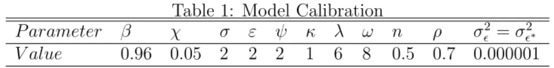
Table 1: Model Calibration

P arameter β χ σ ε ψ κ λ ω n ρ σ2

² =σ2²∗

V alue 0.96 0.05 2 2 2 1 6 8 0.5 0.7 0.000001

between Home and Foreign goods (ω) also vary considerably from as low as 1.107

in Bergin (2002) to 12 (the upper bound in Harrigan (1993)). In the benchmark

model we use ω = 8. Parameter values are summarized in Table 1.

5

Exchange Rate Pass-Through and Exporters

Pric-ing Decisions

5.1

Depreciations due to Home Monetary Expansions

5.1.1 Effects on the Home country

Exchange rate pass-through in the model is determined by a joint response of preset and new prices of exporters. First, suppose the old prices were fixed in producer currency (dollars). When Home money supply increases, they decline in proportion to depreciation as the old cohort gains competitiveness. Since Home real wages also rise, the young exporters are under pressure to set higher re-set prices. However, the increase in new prices is constrained by competitiveness concerns. The net effect on the export price index is therefore negative, but is small due to the opposite movements of the two cohorts’ prices.

If predetermined export prices were fixed in euros, they would not respond to a Home money shock. The new prices would still rise, although by a smaller frac-tion because the absence of expenditure switching contains the increase in Home real wages. Nevertheless, the resulting prediction is surprising: Home export prices should rise when dollar depreciates.

Thus, past invoicing decisions are critical not only in determining the size, but also the sign of the instantenous export prices’ response to Home-generated depre-ciations.

5.1.2 Effects on the Foreign Country

The offsetting effect of the re-set prices that occurs when old prices were set in producer currency does not occur in the Foreign country. In contrast, we find that Foreign export prices respond by more to Home-generated depreciations. This is be-cause 1) foreign exporters face higher demand from Home consumers; and 2) Home money shocks have limited effect on Foreign real wages. As an example, consider the case when old Home exporters follow PCP. Figure 7 documents impulse responses of various variables in both countries to a Home money shock. An imperfect asset market generates deviations from uncovered interest parity and risk sharing at the time of the shock. Unexpected expansion of the Home money supply lowers the Home nominal interest rate with little impact on the foreign interest rate. Thus, the liquidity effect only occurs in the Home country where aggregate demand rises. For-eign exporters’ labor demand rises due to Home consumers’ increased appetite, but foreign nontraded goods producers lose sales due to expenditure switching towards Home’s old exporters.

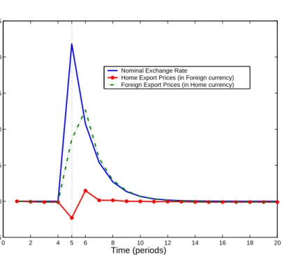
These effects partially offset in equilibrium, and the total demand for foreign labor slightly falls. Real wages in the foreign country therefore fall, but only marginally. With virtually unchanged marginal costs, young exporters in the foreign country are willing to raise their price to meet higher demand at Home. The effect on the Foreign export price index is larger if old foreign export prices were fixed in euros. In both cases, however, the magnitude of the foreign export price response is substantially greater than the response of Home export prices and is always posi-tive. Figure 1 plots relative responses of Home and Foreign export prices to a Home money shock.

To summarize, relative responses of import and export prices to any given ex-change rate depreciation are generally different depending on the origin of the de-preciation. In response to Home-generated depreciations, Home import prices react by more than Home export prices. Moreover, past invoicing decisions are important for the size of instantanous pass-through, as well as the sign of pass-through into

Figure 1: Asymmetric Response of Export Prices to a Home

Money Shock (benchmark model, at−1 =a∗t−1 = 1)

0 2 4 5 6 8 10 12 14 16 18 20 0.99995 1.00000 1.00005 1.00010 1.00015 1.00020 1.00025 Time (periods)

Exchange Rate and Prices

Nominal Exchange Rate

Home Export Prices (in Foreign currency) Foreign Export Prices (in Home currency)

export prices. Next, we discuss firms’ invoicing decisions.

5.2

Is There a Globally Optimal Invoicing Strategy?

Most theoretical studies of individual firms’ invoicing decisions examine a globally optimal invoicing strategy, i.e. when firms always price in one currency. However, in general equilibrium such strategy may not exist, i.e. firms may not always want to follow PCP or LCP but may change their behavior depending on the state of the world. In the Appendix we show that firms profits may be written as:

π_tpcp =Bt · 1 +Et µ³ et+1 et ´_λ¶ Et ³ Wt+1 Wt Φt+1 ´ +covt µ³ et+1 et ´_λ ,Wt+1 Wt Φt+1 ¶¸_1−λ · 1 +Et µ³ et+1 et ´_λ¶ EtΦt+1+covt µ³ et+1 et ´_λ ,Φt+1 ¶¸_−λ (30) π_tlcp=Bt h 1 +Et ³ Wt+1 Wt Φt+1 ´i_1−λ h 1 +Et ³ et+1 et ´ EtΦt+1+covt ³ et+1 et ,Φt+1 ´i_−λ (31) where: Bt = λ −λ (λ−1)1−λWt1−λeλtΩt, Φt+1 =Qt,t+1Ω_Ωt+1_t , and Ωt+j = ¡ PeH∗ t+j ¢_λ−ω¡ P∗ t+j ¢_ω P−1 t+j(1−

n)C∗

t+j.

Next, imagine that firms have perfect foresight. Let dt+1 =

³ et+1

et

´

. Assume also that all covariance terms are zero and that no change is expected in other variables:

Bt = Φt+1 =

³ Wt+1

Wt Φt+1

´

= 1. The profits reduce to:

πpcp _{= 1 +d}λ t+1 πlcp _{= 2}1−λ_{(1 +d}

t+1)λ

The left-side diagram in Figure (2) plots the two functions. Both are convex in expected depreciation, but profits under PCP display greater curvature (since

λ >1). In this case, producer currency pricing is the globally optimal strategy. Figure 2: Price-Setting Firms’ Profits

0.95 0.96 0.97 0.98 0.99 1 1.01 1.02 1.03 1.04 1.05 1.2 1.4 1.6 1.8 2 2.2 2.4 2.6 2.8 3 3.2

Expected Depreciation (e(t+1)/e(t)) PCP LCP 0.95 0.96 0.97 0.98 0.99 1 1.01 1.02 1.03 1.04 1.05 0.8 1 1.2 1.4 1.6 1.8 2 2.2

Expected Depreciation (e(t+1)/e(t))

PCP LCP (Phi*W(t+1)/W(t))=1.04

Now consider a small alteration by assuming that nominal wages are expected to increase by 4 percent:

³ Wt+1

Wt

´

= 1.04. The right-hand side diagram in Figure

(2) plots the resulting profit functions. The graph reveals that the existence of a globally optimal strategy disappears - firms would prefer LCP when they expect

(small levels of11_{) depreciation and PCP otherwise. Note that the last example is}

plausible, because nominal wages are mostly driven by Home money supply, while

the exchange rate is driven byrelative money supplies. Therefore, depending on the

expected paths of the two countries’ money supplies either expected depreciations

or appreciations are possible when Home nominal wages are expected to rise. One can construct similar examples for various values of covariances. Overall, while the full general equilibrium solution requires a numerical approach, the examples above illustrate that invoicing strategies in general equilibrium are likely to be time-varying.

5.3

Profits and Invoicing Under Uncertainty

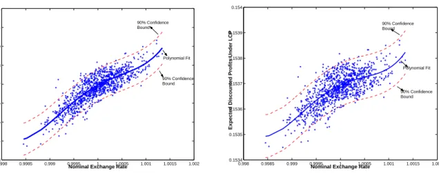
Next we analyze profits in a fully stochastic and dynamic environment. Consider first the benchmark model for the parameters in Table 1. Figure (3) plots simulated observations of the domestic young exporters’ expected discounted profits under PCP and LCP. The average profit functions, obtained through a polynomial fit, have similar shapes under both strategies. They are concave around the long-run equilibrium and display some signs of convexity in times of large depreciations and appreciations.

Figure 3: Average Profit Functions

0.998 0.9985 0.999 0.9995 1 1.0005 1.001 1.0015 1.002 0.1533 0.1534 0.1535 0.1536 0.1537 0.1538 0.1539 0.154 0.1541

Nominal Exchange Rate

Expected Discounted Profits Under PCP

90% Confidence Bound Polynomial Fit 90% Confidence Bound 0.998 0.9985 0.999 0.9995 1 1.0005 1.001 1.0015 1.002 0.1534 0.1535 0.1536 0.1537 0.1538 0.1539 0.154

Nominal Exchange Rate

Expected Discounted Profits Under LCP

90% Confidence Bound

90% Confidence Bound

Polynomial Fit

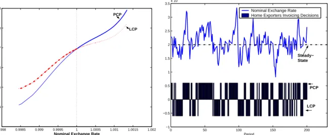
Under LCP the profit function is flatter and with greater curvature. The polyno-mial fits are displayed in the left diagram of Figure (4). Firms’ invoicing strategies are asymmetric: on average, Home exporters tend to choose PCP in times when dollar is depreciated relative to the long-run equilibrium. The opposite is found for LCP (see the right-hand diagram in Figure(3)).

de-Figure 4: Average Profit Functions and Invoicing Decisions 0.998 0.9985 0.999 0.9995 1 1.0005 1.001 1.0015 1.002 0.1534 0.1535 0.1536 0.1537 0.1538 0.1539

Nominal Exchange Rate

Average Expected Discounted Profits (Polynomial Fit)

PCP LCP 0 50 100 150 200 −1 −0.5 0 0.5 1 1.5 2 2.5 3 3.5x 10 −3 Period

Nominal Exchange Rate Home Exporters Invoicing Decisions

PCP

LCP Steady− State

cisions varies with model parameters, and most importantly with λ. For example,

whenλis low (e.g. 3, as opposed to 6 in the benchmark model), the model produces

asymmetry of the opposite direction.

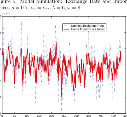
When simulating the model, we observe time-varying and state-dependent rate of exchange rate pass-through. To provide a quantitative assessment relative to the empirical evidence, we take an econometrician’s position. We estimate average pass-through by running a conventional regression of simulated changes in log prices on changes in logs of nominal exchange rates, marginal costs and aggregate consumption demands in the destination markets. For the Home import prices, for example, the estimated equation is:

∆log(P_tef) =α0+α1∆log(et) +α2∆log(MCt∗) +α3∆log(CtF)

In the the benchmark specification with symmetric countries average pass-through into both countries’ import prices is incomplete, as expected. It is roughly equal

to 60%.12 _{Figure (5) plots the simulated nominal exchange rate and Home import}

prices. Next, we discuss the two-types of asymmetries documented in the data.

12_{Since the estimated relationship is very close to the truth in the model, we obtain small}

standard errors and double- and triple-digit t-values on all coefficients. This is why we do not report them.

Figure 5: Model Simulation: Exchange Rate and Import Prices ρ= 0.7, σε=σε∗, λ= 6, ω = 8. 0 50 100 150 200 250 300 350 400 450 500 −1.5 −1 −0.5 0 0.5 1 1.5x 10 −3

Nominal Exchange Rate Home Import Price Index

5.4

Directional Asymmetry: Depreciations vs.

Apprecia-tions

Coughlin and Pollard (2000) document different responses of U.S. import prices de-pending on the direction of exchange rate movements. They find that in times of persistent dollar depreciations higher pass-through is more likely across industries. Wickermasinghe and Silvapulle (2003) also find statistically significant asymmetric response of Japanese manufacture import prices. However, their findings are op-posite to Coughlin and Pollard’s: import prices in Japan were found to respond by more when yen appreciates. We now discuss how these directional asymmetries could arise in the context of our model.

The asymmetric invoicing decisions, discussed above, are the main reason for asymmetric pass-through in the model. When the dollar appreciates for several consecutive periods and Home firms price in local currency, aggregate pass-through is entirely due to the changes in new prices. The latter are mostly driven by changes in marginal costs and foreign demand.

Table 2: Directional Asymmetry of Pass-Through into Im-port Prices (λ) Depreciations Appreciations 2 0.5122 0.6562 3 0.5228 0.6789 6 0.6810 0.4794 10 0.6374 0.4914

PCP and experience expenditure switching towards their goods. Pass-through elas-ticity is determined by the difference between the rate of depreciation and percentage change in new prices. Re-set prices in this cases are affected by two opposing factors: higher marginal marginal costs and competitiveness loss to the ”old” exporters. In times of persistent depreciations marginal costs (Home wages) rise by more because expenditure switching raises demand for Home labor. On the other hand, loss of competitiveness contains the increase in new prices. Thus, whether pass-through is higher or lower in times of depreciations depends critically on the strength of ex-penditure switching towards ”old” firms. The latter, in turn, is mostly determined

by the elasticity of substitution, λ. When markets are close to being competitive

(low monopoly power, highλ) market share concerns are important,and new export

prices rise by less in times of depreciations. Put differently, when λ is high, we

should expect import prices to respond by more in times of depreciations.

Table 2 presents model-implied pass-through rates in times of persistent

de-preciations and apde-preciations 13 _{for several values of λ. In the benchmark model}

with λ = 6 pass-through into the Home import prices is higher in times of dollar

depreciations (≈ 68%) than in times of appreciations (≈ 48%). This is consistent

with the findings in Coughlin and Pollard (2000). On the other hand, when we set

λ= 3, asymmetry changes: pass-through into Home import prices is higher in times

of appreciation, consistent with Wickermasinghe and Silvapulle (2003). Overall, the model predicts that countries with less monopolistic markets should observe higher pass-through into import prices in times of depreciation and lower pass-through in

13_{Since we assume two-period price stickiness, we define depreciations as persistent when they}

times of appreciation.

5.5

Origin-Based Asymmetry: Export vs. Import Prices

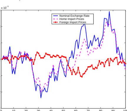
Second type of asymmetry, reported in Dwyer et. al. (1993) is the difference in pass-through rates into export vs. import prices. Since our model has only two countries, this asymmetry can also be stated as different pass-through rates into import prices across countries. The intuition of how such asymmetry can arise in the model has been discussed in the context of the effects of Home country shocks on Foreign export prices (see section 5.1). There,

Figure 6: Model Simulation: Exchange Rate and Prices,

ρ= 0.9, σ2ε σ2 ε∗ = 10 0 10 20 30 40 50 60 70 80 90 100 −3 −2 −1 0 1 2 3x 10 −3

Nominal Exchange Rate Home Import Prices Foreign Import Prices

it was found that depreciations caused by domestic monetary expansions produce a larger response by import prices. Since the exchange rates in the model are

determined byrelative money supply shocks, a country with a more variable money

supply should observe higher average pass-through rate into its import prices. This conclusion is similar to that of Devereux, Engel and Storgaard (2002), although our motivation is somewhat different. In their model low variance of Home money shocks stabilizes marginal costs relative to the variability of the exchange rate, making PCP

Table 3: Origin-Based Asymmetry: Pass-Through into Import and Export Prices

Relative Money Shocks Variability

³ σε∗

σε

´

Home Export Prices Home Import Prices

1 -0.6041 0.6041 1.5 -0.6617 0.4897 2 -0.6941 0.4670 6 -0.8382 0.2222 10 -0.8993 0.1367 15 -0.9394 0.0423

a preferred strategy for Home exporters and raising relative pass-through in the Foreign economy. In our setting, although low variance of domestic money supply also lowers correlation between exchange rates with marginal costs, it also raises the correlation of the aggregate demand in the Foreign country with the nominal exchange rate. In addition, it does not necessarily imply PCP as a more preferred strategy.

To quantify this asymmetry, in Table 3 we report estimated pass-through rates under different relative standard deviations of money supply shocks. In one extreme case, when the standard deviation of Foreign money supply shocks is 10 times larger that of the Home country, pass-through into export prices rises to almost 90%, while for import prices it drops to less than 14%. Figure (6) displays the simulated export and import price series for this extreme case.

6

Conclusion

In this paper we have examined a two-country new open economy macroeconomics

model with two-period price stickiness ´a la Taylor, where exporters’ choice of

cur-rency in which to fix prices is endogenous. The model predicts an incomplete pass-through of exchange rate shocks into import and export prices. In addition, we have arrived at four main findings.

and appreciation. In the benchmark model, exporters choose producer currency pricing when exchange rate is depreciated relative to its long-run equilibrium level and producer currency pricing when it is appreciated.

Second, when exchange rate depreciation is caused by a domestic monetary ex-pansion, the response of Home country export price index is muted, even when the pre-set prices are fixed in producer currencies. This result is due to the offsetting movements of the pre-set and re-optimized prices.

Third, instant pass-through of exchange rate shocks into import and export prices is asymmetric. Depreciations caused by the Home country monetary expan-sions produce larger responses of import prices than export prices.

Fourth, average pass-through displays two types of asymmetries, also found in the data. First is the directional asymmetry: in times of depreciation, a country with a more competitive market should observe higher pass-through into import prices than in times of appreciation. Second is the origin-based asymmetry: a coun-try with a more variable money supply should observe higher pass-through into its import prices.

The model and findings presented in this paper suggest several directions for future research, both empirical and theoretical. On the theoretical front, the pro-posed setting is well suited for analyzing optimal monetary policy in an international setting. The endogenous nature of exchange rate pass-through in a fully dynamic setting is an advantage over models that take the pass-through rate as given. As Devereux et. al. (2002) point out, it is inconsistent to analyze monetary policy for a given level of pass-through, when pass-through itself depends on monetary pol-icy. Furthermore, the model could be improved in several dimensions. We do not model a distribution sector, which many argue is important for reconciling low pass-through into consumer prices and higher pass-pass-through into export supply prices,

which is also observed in the data14_{. A more elaborate analysis should also include}

more determinants of nominal exchange rates, such as productivity shocks. Another

interesting direction is to incorporate capital into the model to examine the business

cycle properties of the model15_.

Finally, it would be useful to perform more empirical research to shed light on the virtually unexplored issue of asymmetric pass-through and firms’ invoicing decisions.

15_{Kollman (2003) constructs an international business cycle model in the new open economy}

style, but assumes local currency pricing. The role of endogenous exchange rate pass-through on the business cycle properties of NOEM models has not been explored by researchers.

References

[1] Bergin, Paul, 2002, ”How Well Can the New Open Economy Macroe-conomics Explains the Exchange Rate and Current Account?”, mimeo, University of California at Davis; also NBER working paper w10356. [2] Bachetta, Philippe, and Eric van Wincoop, 2002, ”A Theory of

Cur-rency Denomination of International Trade”, forthocoming, Journal of International Economics.

[3] Betts, Caroline, and Michael B. Devereux, 1996, The Exchange Rate in a Model of Pricing to Market, European Economic Review, 40, 1007-1021.

[4] Betts, Caroline, and Michael B. Devereux, 2000, Exchange Rate Dy-namics in a Model of Pricing to Market, Journal of International Eco-nomics, 50, 215-244.

[5] Campa, Jos´e Manuel, and Linda S. Goldberg, 2002, Exchange Rate Pass-Through into Import Prices: A Macro or Micro Phenomenon?, National Bureau of Economic Research, working paper no.8934

[6] Campa, Jos´e Manuel, and Jos´e M. Gonz´alez, 2002, Differences in Ex-change Rate Pass-Through In the Euro Area, International Center for Financial Research, Research paper no.479

[7] Clarida, Richard, H. The Empirics of Monetary Policy Rules in Open Economies, National Bureau of Economic Research, working paper no.8603

[8] Chari, V.V., Patrick J. Kehoe, and Ellen R. McGrattan, 2000, Can Sticky Price Models Generate Volatile and Persistent Real Exchange Rates?, Staff Report 277, Federal Reserve Bank of Minneapolis. [9] Corsetti, Giancarlo, and Paolo Pesenti, 2001, International Dimensions

of Optimal Monetary Policy, National Bureau of Economic Research, working paper no.8230

[10] Coughlin, Cletus, C., and Patricia S. Pollard, Exchange Rate Pass-Through in U.S. Manufacturing: Exchange Rate Index Choice and Asymmetry Issues, Federal Reserve Bank at St. Louis, Working Paper 2000-022A.

[11] Coughlin, Cletus, C., and Patricia S. Pollard, Size Matters: Asym-metric Exchange Rate Pass-Through At The Industry Level Federal Reserve Bank at St. Louis, Working Paper 2003-029B.

[12] Devereux, Michael B., Charles Engel and Peter E. Storgaard, 2002, Endogenous Exchange Rate Pass-Through when Nominal Prices are Set in Advance, forthcoming, Journal of International Economics.

[13] Devereux, Michael B., Charles Engel, Monetary Policy in the Open Economy Revisited: Exchange Rate Flexibility and Price Setting Be-havior, 2003, forthcoming, Review of Economic Studies.

[14] Dixit, A. K., and J. E. Stiglitz, 1977, Monopolistic competition and optimum product diversity, American Economic Review,67, pp. 297-308

[15] Dwyer, Jacqueline, Christopher Kent, and Andrew Pease, Exchange Rate Pass-Through: The Different Responses of Importers and Ex-porters, May 1993, Economic Research Department, Federal Reserve Bank of Australia, Research Discussion Paper no. 9304

[16] Engel, Charles, Expenditure Switching and Exchange Rate Policy, NBER Macroeconomics Annual 2002, no. 17, 231-272.

[17] Engel, Charles, and John H. Rogers, 2002, How Wide is the Border? American Economic Review, 86, 1112-1125.

[18] Faruqee, Hamid, 2004, Exchange Rate Pass-Through in the Euro Area: The Role of Asymmetric Pricing Behavior, IMF Working Paper, no. WP/04/14, January 2004.

[19] H¨ufner, Felix, P., and Michael Schr¨oder, 2002, Exchange Rate

Pass-Through to Consumer Prices: A European Perspective, Center for European Economic Research, Discussion Paper no. 02-20

[20] Kenny, Geoff and Donald McGettigan, Exchange Rate Pass-Through and Irish Import Prices, Research Technical Paper no. 6/RT/96, Cen-tral Bank of Ireland, December 1996.

[21] Knetter, Michael, M., 1989, Price Discrimination by U.S. and German Exporters, American Economic Review, 79, 198-210

[22] Knetter, Michael, M., 1993, International Comparisons of Pricing-to-Market Behavior, American Economic Review, 83, 473-486

[23] Kollman, Robert, 2002, Monetary Policy Rules in the Open Economy: Effects on Welfare and Business Cycles, Carnegie-Rochester Confer-ence Series on Public Policy.

[24] Kollman, Robert, 2003, Monetary Policy Rules in an Interdependent World, mimeo, Department of Economics, University of Bonn.

[25] Krugman, Paul, 1987, Pricing to Market when the Exchange Rate Changes, in S.W. Arndt and J.D. Richardson, eds., Real-Financial Linkages Among Open Economies, Cambridge, MIT Press.

[26] Lane, Philip R., 2001, The New Open Economy Macroeconomics: A Survey, Journal of International Economics, 54, 235-266.

[27] Menon, Jayant, Exchange Rate Pass-Through, Journal of Economic Surveys, Vol. 9, No. 2, 1995.

[28] Miranda, Mario J. and Paul L. Fackler, 2002, Applied Computational Economics and Finance, MIT Press.

[29] Obstfeld, Maurice, 2002, Exchange Rates and Adjustment:

Perspec-tives from the New Open Economy Macroeconomics Center for

Inter-national and Development Economics Research. Paper C02-124.

[30] Obstfeld, Maurice, and Kenneth Rogoff, 1995, Exchange Rate Dynam-ics Redux, Journal of Political Economy, 103, 624-660

[31] Obstfeld, Maurice, and Kenneth Rogoff, 1996, Foundations of Interna-tional Macroeconomics, MIT Press.

[32] Obstfeld, Maurice, and Kenneth Rogoff, 1998, Risk and Exchange Rates, National Bureau of Economic Research, working paper no.6694 [33] Obstfeld, Maurice, and Kenneth Rogoff, 2000, New Directions for Stochastic Open Economy Models, Journal of International Economics, 50, 117-153

[34] Obstfeld, Maurice and Kenneth Rogoff, The Six Major Puzzles in In-ternational Finance: Is There a Common Cause?, in Bernanke, Ben S., and Kenneth Rogoff, eds., NBER Macroeconomics Annual, 15 (2000). [35] Olivei, Giovanni, P. Exchange Rates and the Prices of Manufactured Products Imported into the United States, New England Economic Review, First Quarter, 2002.

[36] Sarno, Lucio, Toward a new paradigm in open economy modeling: where do we stand?, The Regional Economist, 2001, issue May, pp. 21-36. Also available in Federal Reserve Bank of St. Louis Review, May/June 2001.

[37] Schenk, Andrea, 2003, Exchange Rate Pass-Through into Canadian Import Prices, mimeo, Queen’s University.

[38] Wickremasinghe, Guneratne and Param Silvapulle, 2003, Exchange Rate Pass-Through to Manufactured Import Prices: The Case of Japan, mimeo, Monash University.

A

Exporters Profits

Here we show how to equations (30)-(31) were derived.

A.1

PCP Profits

The price-setting problem is given by: max PeH pt πpcp_t =Et 1 X j=0 Qt,t+j à PeH pt −Wt+j Pt+j ! à PeH pt et+jPteH+j∗ !−λà PeH∗ t+j P∗ t+j !−ω (1−n)C∗ t+j= =¡PeH pt ¢1−λ  _Et 1 X j=0 Qt,t+jeλt+jΩt+j  ₋¡_PeH pt ¢−λ  _Et 1 X j=0 Qt,t+jWt+jeλt+jΩt+j   where Ωt+j= ¡ PeH∗ t+j ¢λ−ω¡ P∗ t+j ¢ω P_t−₊1_j(1−n)C∗

t+j.The re-set price is given by:

PeH pt = λ λ−1 Et 1 P j=0 Qt,t+jWt+jeλt+jΩt+j Et 1 P j=0 Qt,t+jeλt+jΩt+j

Plugging the optimal price into the profit function and re-arranging yields:

π_tpcp= λ −λ (λ−1)1−λ " Et 1 P j=0 Qt,t+jWt+jeλt+jΩt+j #1−λ " Et 1 P j=0 Qt,t+jeλt+jΩt+j #−λ

Taking the current period values outside of each bracket, we obtain:

π_tpcp= λ−λ (λ−1)1−λ ¡ WteλtΩt ¢1−λ ¡ eλ tΩt ¢−λ · 1 +Et µ Qt,t+1W_Wt+1_t ³ et+1 et ´λ_Ω t+1 Ωt ¶¸1−λ · 1 +Et µ Qt,t+1 ³ et+1 et ´λ_Ω t+1 Ωt ¶¸−λ

To save space, denote: Bt = λ

−λ

(λ−1)1−λWt1−λeλtΩt and Φt+1 = Qt,t+1Ω_Ωt+1_t . Expanding the

expectational terms, we obtain:

πtpcp=Bt · 1 +Et µ³ et+1 et ´λ¶ Et ³ Wt+1 Wt Φt+1 ´ +cov µ³ et+1 et ´λ ,Wt+1 Wt Φt+1 ¶¸1−λ · 1 +Et µ³ et+1 et ´λ¶ EtΦt+1+cov µ³ et+1 et ´λ ,Φt+1 ¶¸−λ

A.2

LCP Profits

Next, re-do the same exercise for the case of LCP. The price-setting problem is given by: max PeH∗ lt πtlcp=Et 1 X j=0 Qt,t+j µ et+jPlteH∗−Wt+j Pt+j ¶ à PeH∗ lt PeH∗ t+j !−λà PeH∗ t+j P∗ t+j !−ω (1−n)Ct∗+j= =¡PeH∗ lt ¢1−λ  _Et 1 X j=0 Qt,t+jet+jΩt+j  ₋¡_PeH∗ lt ¢−λ  _Et 1 X j=0 Qt,t+jWt+jΩt+j  

Optimal price: PeH∗ lt = λ λ−1 Et 1 P j=0 Qt,t+jWt+jΩt+j Et 1 P j=0 Qt,t+jet+jΩt+j

Plug optimal price into the profits:

πlcp_t = λ−λ (λ−1)1−λ " Et 1 P j=0 Qt,t+jWt+jΩt+j #1−λ " Et 1 P j=0 Qt,t+jet+jΩt+j #−λ = = λ−λ (λ−1)1−λ (WtΩt)1−λ (etΩt)−λ h 1 +EtQt,t+1W_Wt+1_t Ω_Ωt+1_t i1−λ h 1 +EtQt,t+1et_e+1_t Ω_Ωt+1_t i−λ

Finally, expanding the expectational term:

πtlcp=Bt h 1 +Et ³ Wt+1 Wt Φt+1 ´i1−λ h 1 +Et ³ et+1 et ´ EtΦt+1+cov ³ et+1 et ,Φt+1 ´i−λ

B

Figure 7. Impulse Responses of Selected

Vari-ables

(Responses are to a positive Home Money Shock. Benchmark model,ρ=0.5,at−1=a∗t−1= 1.)

0 2 4 6 8 10 12 14 16 18 20 0.9999 1 1 1.0001 1.0001 1.0002 1.0002 1.0003 1.0003 1.0004

Impulse Response to a Home Shock: Nominal Wages

Home Foreign 0 2 4 6 8 10 12 14 16 18 20 0.9999 1 1 1.0001 1.0001 1.0002 1.0002 1.0003 1.0003 1.0004

Impulse Response to a Home Shock: Real Wages

Home Foreign 0 2 4 6 8 10 12 14 16 18 20 0.994 0.995 0.996 0.997 0.998 0.999 1 1.001

Impulse Response to a Home Shock: Nominal Interest Rates

0 2 4 6 8 10 12 14 16 18 20

1 1.00005 1.0001

Impulse Response to a Home Shock: Consumptions

Home Foreign 0 2 4 6 8 10 12 14 16 18 20 0.99994 0.99996 0.99998 1.00000 1.00002 1.00004 1.00006 1.00008 1.00010 1.00012 1.00014

Impulse Response to a Home Shock: Home Country Labor

Exporters Labor Demand Nontraded Goods Firms Labor Demand Per Capita Labor Supply

0 2 4 6 8 10 12 14 16 18 20 0.99990 0.99995 1.00000 1.00005 1.00010 1.00014

Impulse Response to a Home Shock: Foreign Labor

Exporters Labor Demand Nontraded Goods Firms Labor Demand Per Capita Labor Supply