Competition in the U.S. Mutual Fund Industry: A performance evaluation of actively managed domestic equity mutual funds

(1)

LUND UNIVERSITY SCHOOL OF ECONOMICS AND MANAGEMENT

Department of Economics

Bachelor´s Thesis within Financial Economics Spring 2017

Competition in the U.S. Mutual Fund Industry

A performance evaluation of actively managed domestic equity mutual funds

Adam Öster

Abstract

I evaluate a total of 204 U.S. equity mutual funds split into one major group and one additional group for the time period 2002-2016. The major group consists of the ten largest U.S. mutual fund families based on AUM while the additional group consists of a sample of the remaining operative U.S. mutual fund families. The major group manages 58% of U.S. mutual fund supply, thus indicating a non-competitive market structure. By comparing the performances of these two particular groups, I investigate whether the current market structure within the U.S. mutual fund industry is beneficial from the point of view of U.S. investors. That is, is their aggregated private wealth efficiently invested considering that as few as ten U.S. mutual fund families are managing the majority of it? Or would they experience an increased yield if they rather reallocated it into the additional fund families? Moreover, I benchmark the performance of each group to adequate market indices in order to investigate whether the active management pays off. I find that out of my 28 regressions, eight yield alphas statistically significantly different from zero at the 1% level. Additionally, when comparing each group´s mean alpha to each other, I find a statistically significant difference for large value stocks net of fees to a significance of 99%. These findings combined suggest that the major group perform superior to the additional group and which accordingly justifies the fact that the major group manage the majority of U.S. mutual fund supply. My findings further support the fact, although with varying levels of statistical significance, that the active management by the two groups is generally not worth paying for since the fees exceed the beta-adjusted excess returns, interpreted as the actively managed mutual funds outperform the market on a gross level but once the fees are paid the net alphas inversely underperform the market. This tendency within the performance of mutual funds is in line with previous research.

Keywords: Performance evaluation, equity mutual fund, CAPM, Jensen´s alpha, OLS regression

(2)

Acknowledgements

I wish to thank my supervisor Emre Aylar for valuable criticism. I am also grateful to Julia Sahlin at Morningstar Sweden for providing necessary mutual fund data. Lastly, Judy Steenstra at the Investment Company Institute (ICI) is acknowledged for her appreciated insight into the U.S. mutual fund industry.

Österlen in August 2017 Adam Öster

(3)

1. Introduction

Over the past several decades, the mutual fund industry has been associated with the so-called “active-versus-passive debate”. The fundamental of this debate concerns the disagreement on the true interpretation of active management. Some mutual fund managers have been proved to very closely track certain benchmark indices in terms of stock-picking replication while still marketing the fund as being actively managed (Cremers & Petajisto, 2009). By doing so, the manager almost completely eliminates the probability of outperforming the market while still obtaining investor fees for “active” management. The manager therefore basically gets paid for passive management, i.e. a profitable strategy for the fund family but at the expense of the investors´ private wealth. This is in clear contrast to how the U.S. Securities and Exchange Commission (SEC) (2017) expresses it when advising investors: “Don´t let someone else live the life you´ve been saving for”. Such a strategy explained above has become increasingly implemented by mutual fund managers and also has it been given the name “closet indexing”. Consequently, attempts to identify closet indexers have been made through different measurements such as tracking error1_{and active share}2_{(Cremers & Petajisto, 2009). The fact that investors pay for a}

service they may not receive, and more importantly often do so without being aware of it, is indeed serious.

This study will touch upon the active-versus-passive debate by evaluating the performance of U.S. mutual funds. Unlike previous studies though, I will focus on the performance of major U.S. mutual fund families. More precisely, I will compare the historical performance of major U.S. mutual fund families to their additional peers during a time period of 15 consecutive years, starting from 2002 until 2016. The definition of “major” is based on each family´s assets under management (AUM).3_{According to}

data retrieved from the Investment Company Institute (ICI) (2017) as of year-end 2016, the top ten4_{major U.S. mutual fund families are together managing 58% of total assets invested in U.S.}

mutual funds (Waggoner, 2016). These ten families will represent my major fund group while the additional fund group consists of a sample of the remaining U.S. mutual fund families. I have not been able to identify the total number of operative fund families in the U.S.5_{, but according to}

Judy Steenstra at the ICI there are at least 200. The reason why I consider this comparison of groups to be of interest is due to the potential oligopolistic market structure which they

1_{Measures how closely the fund tracks its benchmark index by computing the standard deviation of the difference}

between fund returns and index returns. The higher the value, the more actively managed is the fund.

2_{Measures how much of the stock holdings as well as their allocation within the fund that deviate from its}

benchmark index. A high percentage corresponds to a high deviation and thus an indication of high active management.

3_{Total market value of all assets managed by the fund, i.e. a measure of fund size.} 4_{See Appendix A.}

(6)

2

represent. If the major group turns out to underperform the additional group, this would demonstrate an inefficient allocation of U.S. wealth since these ten families together manage the majority of U.S. fund supply but yet perform inferior to the additional market participants. Therefore, my initial objective is to investigate whether the major fund families really deserve such a dominant market position within the U.S. mutual fund industry by comparing both groups´ past performances. To my knowledge, such a comparison has not been conducted before. I will evaluate solely actively managed U.S. domestic equity mutual funds6_{of which all are}

open-ended.7_{My study is primarily addressed to U.S.}_retail_investors8_{rather than to U.S.}

institutional investors9_{since the former most likely represent those that are being exploited due to}

ignorance regarding mutual funds. From an U.S. retail investor point of view, AMUSDEMFs are indeed an appropriate type of mutual fund to evaluate because as of mid-2016, 43.6% of U.S. households owned them. Additionally, 89% of total U.S. mutual fund assets as of year-end 2016 were held by U.S. households and 52% of these assets represented U.S. equity funds, where domestic holdings dominated (Investment Company Institute, 2017). This overrepresentation by households may partly be explained by the fact that U.S. citizens tend to save for education (college) as well as for retirement primarily through mutual funds. Furthermore, I will benchmark each of the two groups to adequate market indices in order to confirm whether the active management really pays off. That is, do my AMUSDEMFs outperform the market during the studied time period or do they in fact perform in line with passively managed funds (i.e. index funds), or perhaps worse? In accordance with the efficient market hypothesis (EMH)10_{, actively managed funds do not yield}

superior returns to the index regardless of whether technical11_{, fundamental}12_{, or any other}

analysis is applied. Thus, if the market is strongly efficient, neither of my two fund groups would be able to beat the market over time.

Based on data provided by Morningstar, I will evaluate a total of 204 AMUSDEMFs. Alphas13

will be computed and interpreted as the performance measurement of the fund managers´

6_{Henceforth, these particular funds will be given the abbreviation AMUSDEMFs.}

7_{The most common kinds of mutual funds and which give the investor the possibility to easily purchase and sell}

unlimited shares to a low cost (Bodie, Kane & Marcus, 2014).

8_{i.e. individual investors/households.}

9_{i.e. professional investors such as investment firms or similar.}

10_{Financial theory assuming the existence of market efficiency, interpreted as the stock price reflecting and}

incorporating all available information. Stocks therefore never trade when being over or undervalued since they have already regressed to their fair value at the time of the purchase. There are three degrees of efficiency: weak, semi-strong, and strong (Fama, 1970). The theory is controversial where on the one hand academics tend to embrace it while on the other hand practitioners generally oppose it.

11_{Forecasts of stock prices are based on historical patterns in data}_{(Bodie, Kane & Marcus, 2014).}

12_{Forecasts of stock prices are based on the firm´s financial statements (e.g. assets and liabilities) as well as on}

market factors (e.g. interest rates and gross domestic product (GDP))(Bodie, Kane & Marcus, 2014).

13_{Also known as Jensen´s alpha (α). This corresponds to the risk-adjusted excess return (or abnormal return) on the}

(7)

3

picking ability.14_{My fund samples are additionally split into subsamples in order to correspond to}

each combination of investment style (value, blend, growth) as well as market capitalization (small, medium, large).15_{I will run 28 ordinary least squares (OLS) regressions using the}

regression equation applied to the capital asset pricing model (CAPM). The results are subsequently tested for statistical significance. Lastly, robustness checks concerning the reliability of my data are conducted and include tests for heteroscedasticity, autocorrelation, stationarity, normally distributed data, as well as for regression specification error.

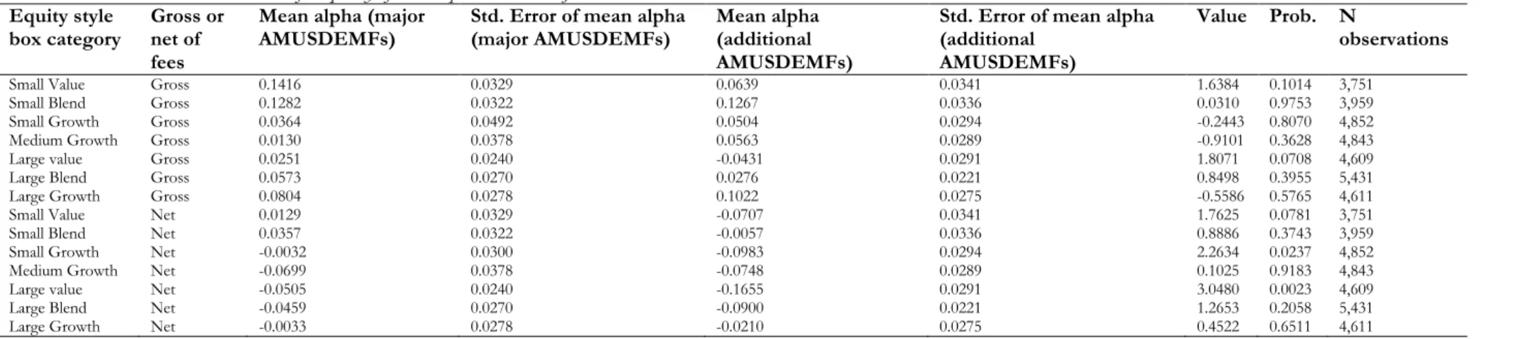
I find that out of my 28 regressions, 20 yield alphas statistically insignificantly different from zero at the 1% significance level, thus indicating a performance by the two fund groups equalling that to the market. Eight regressions do however yield non-zero alphas to a significance of 99% where three of these correspond to the major fund group yielding positive gross alphas for small value, small blend, as well as large growth stocks. The remaining five regressions correspond to the additional fund group yielding positive gross alphas for small blend as well as large growth stocks whilst yielding negative net alphas for small growth, large value, as well as large blend stocks. Neither fund group yields positive net alphas of statistical significance. When comparing each group´s mean alpha to each other, I do find only a statistically significant difference at the 1% level for large value stocks net of fees, and where the major group performed the superior mean alpha. These performances combined suggest that the major group outperforms the additional group and which accordingly justifies the fact that the major group manages the majority of U.S. mutual fund supply. Concerning the active management, my findings do support the fact, although with varying levels of statistical significance, that it is generally not worth paying for the 204 AMUSDEMFs since the fees exceed the beta-adjusted excess returns. That is, the fund managers yield positive gross alphas which turn into negative net alphas once the fees are paid. Lastly, my time series data are stationary and have been adjusted for heteroscedasticity as well as autocorrelation. However, eight of my regressions have been tested positive for specification error at the 1% significance level.

My study is organised as follows. In the upcoming chapter I will begin with a review of what have previously been studied within my chosen topic. Next, my data samples (mutual funds, stock market indices, risk-free interest rate) are presented alongside the hypothesis. In Chapter 4, methodology and theory (including CAPM, Jensen´s alpha, and econometric approach) are highlighted, followed by results and analysis as well as a subsequent conclusion and discussion in

14_{Also known as (security) selection ability.} 15_{I will discuss this procedure further in Chapter 3.}

(8)

4

Chapter 5 and 6, respectively. Lastly, Chapter 7 will contain a discussion regarding recognised limitations affecting my study as well as suggestions for future research.

(9)

5

2. Literature Review

Studies of performance evaluation of mutual funds, and in particular U.S. mutual funds, are by no means unique to the field of finance. Plenty of literatures have been published over the years and I will therefore review solely a range of those that may be considered to be as closely related to my particular study within performance evaluation as possible.

Starting with a review of the active-versus-passive debate, empirical evidence points at a divergence between performances of active management. On the one hand, (Gruber, 1996; Jensen, 1967; Malkiel, 1995; Sharpe, 1966) find that actively managed funds do in fact underperform the market. On the other hand, (Grinblatt & Titman, 1993; Wermers, 2000) are able to prove the opposite. However, taking this divergence into consideration, there may be more evidence inclining that active management does not yield superior returns to a passively managed portfolio, at least not net of fees. Those studies presented above differ from each other in terms of approach, performance measurement, sample size, time span etc. but their resemblance is however to evaluate the performance of actively managed U.S. equity funds. Gruber (1996) asks himself why investors keep pouring money into funds which over time constantly underperform. He concludes that future performance can in fact be predicted by past performance and this is exactly what investors are pursuing when identifying previously outperforming funds. In contrast to many other studies, both Gruber (1996) and Malkiel (1995) are accounting for survivorship bias16_{and they are thereby avoiding a misinterpreted persistence}

of performance with the consequence of overestimating the fund manager´s stock-picking ability. Yet, Grinblatt and Titman (1993) does not find any evidence of passive management outperforming active management whilst accounting for survivorship bias. Despite those significantly positive risk-adjusted returns obtained in the study, it should however be mentioned that the authors do not rule out the possibility of underperforming the market net of fees. Moreover, Wermers (2000) emphasises the negative impact of fees on performance where he finds that those equity holdings included in his fund sample did outperform the market by an average of 1.3% per annum when being gross of fees. On a net return basis however, the funds were unable to beat the market when underperforming with a 1% per annum. Consequently, the fees exceeded the additional returns generated by the active management and thus made the investors to pay for a service they did not receive. Sharpe (1966) draws similar conclusions regarding the relationship between fee and fund performance where he summarises it as “good performance is associated with low expense ratios” (Sharpe, 1966, p. 132). Both Jensen (1967)

16_{Unsuccessful funds may be closed down by managers in order to not negatively affect the overall performance by}

(10)

6

and Malkiel (1995) were unable to obtain returns which outperformed the market, regardless of whether returns gross or net of fees were computed.

In a quite recent study composed by Flam and Vestman (2014), similar conclusions as to those regarding the mutual fund performance in the U.S. can be drawn in the Swedish mutual fund industry. Flam and Vestman (2014) evaluates 115 actively managed equity funds as well as 15 equity index funds during the time period from 1999 to 2009. The average net excess return among the equity funds has been negative and the variation between them was quite substantial where the top fund yielded a net excess return of 13.6% per annum and the bottom fund -15.3% per annum. The average gross excess return was however positive, equalling 0.9% annually. Although more than half of the actively managed equity funds yielded positive gross excess returns, Flam and Vestman (2014) concludes that any evidence of true stock-picking skills among the Swedish fund managers could not be confirmed due to the lack of persistence of returns. Consequently, their performance may as well have been the result of pure luck. Regardless of stock-picking skills or not, the investors did not benefit from the active management since the net excess return was on average negative.

As far as I am aware, the only comparable approach to the one taken in my study regarding performance evaluation of groups of mutual fund families, and with the intention to investigate for an inefficient industry concentration, has been conducted by Dahlberg (2015). He depicts the mutual fund industry in Sweden as being dominated by the four largest banks17_{based on AUM,}

thus indicating an oligopolistic market structure similar to that in the U.S.18_{It turns out that}

almost each and one of those funds managed by the four banks has underperformed both its benchmark index as well as many of those funds managed by their additional peers.19

Additionally, evidence point at the fact that some of these funds are suspiciously close to certain indices in terms of stock-picking replication that one may question whether closet indexing have been practiced. As a journalist, Dahlberg (2015) conducts interviews with a number of distinguished characters within the financial sector (e.g. William F. Sharpe) in order to obtain different perspectives. Based on these interviews, it appears as if the four banks have misled investors in order to benefit from those funds then chosen by the investors. The banks have subsequently escaped from giving proper advice about these particular funds´ past performances as well as appropriateness to actually invest in. Dahlberg (2015) aims to make investors react

17_{Nordea, Skandinaviska Enskilda Banken (SEB), Svenska Handelsbanken (SHB), Swedbank.}

18_{A concentration within the}_banking_{industry is to be found in the U.S. too, consisting of J.P. Morgan Chase & Co,}

Wells Fargo & Co, Bank of America, and Citigroup (Federal Reserve, 2016). However, among these banks only J.P. Morgan Chase & Co is also qualified to represent the top ten U.S. mutual fund families.

(11)

7

against the four banks´ inability to perform superior to the market as well as to many of their competitors while still managing to maintain such a dominant market position. He calls on the investors to reallocate their wealth into those fund families which do perform and accordingly cease the contribution of benefitting the poorly performing banks.

My study is based on the CAPM framework. Complements to this single-factor model (with market risk20_{as the one factor) are multi-factor models such as Fama-French (1993)}

three-factor21_{as well as Carhart (1997) four-factor}22_{models. Arguments claiming that more factors}

included in the model increase the explanatory power of the computed returns may be justified. However, Flam and Vestman (2014) apply all these factor models in their study and they find no evidence of any significant differences in returns. Additionally, as mentioned in the previous chapter, I will split my mutual fund data into subsamples in order to account for differences in stocks similarly to the multi-factor models.

20_{Also known as beta (β). This risk arises from macroeconomic conditions such as repo rates, state of the economy}

etc. Through economic policy, market risk can be reduced but not entirely eliminated (Bodie, Kane & Marcus, 2014).

21_{This model adds another two factors to the initial market risk-factor. These are firm size (SMB) and the firm´s}

price-to-book (P/B) ratio (HML). SMB stands for “Small Minus Big” and is interpreted as the difference in returns between small- and large-sized firms (i.e. market capitalization). HML stands for “High Minus Low” and is interpreted as the difference in returns between value and growth stocks (i.e. investment style) where a high value corresponds to value stocks (high P/B ratio) and a low value corresponds to growth stocks (low P/B ratio). Small value stocks have tended to outperform the market over time and those two factors added here are able to distinguish between stocks in such a way that it will benefit the entire model used for performance evaluation.

22_{This is an extension of the three-factor model containing the additional factor “monthly momentum” (MOM).}

MOM captures the tendency of the stock price to keep increasing after its initial increase or vice versa, i.e. a momentum effect.

(12)

8

3. Data

23

_{and Hypothesis Development}

The time series data in this chapter are separated into three sections. Morningstar provides the mutual fund data. Bloomberg (via LINC Lund) provides the Russell index series. The U.S. Treasury bill rates can be obtained on the official website of the Federal Reserve Bank of St. Louis (2017). The mutual funds as well as the index series consist of cumulative returns on a monthly basis ranging from 01/01/2002 to 12/30/2016. The Treasury bills share the equivalent time span. A motivation to the choice of this particular time period follows by the fact that it is long enough to enable the evaluation of persistence of performance achieved by the fund managers. Additionally, it does include the financial crisis of 2007-2008 which will highlight how well the managers were able to stock-pick during those turmoil markets which occurred at that particular time. My studied time period is further split into three sub periods24_{in order to more accurately}

investigate the managers´ persistence over time as well as to identify potential impact of market disturbances on performance throughout these 15 years, including the latest financial crisis mentioned above.

3.1 Mutual Funds

My selected AMUSDEMFs are listed in Appendix B and C, respectively. According to Table 9.1, there are 70 major as well as 134 additional funds in my study, together consisting of a total of 32,056 observations.

[Table 9.1]

Now, the selection process of these funds is rather comprehensive. I will go through it thoroughly using a step-by-step approach. First of all, in line with what was stated in the introduction, this study will entirely focus on those funds that share the characteristics of being open-ended, actively managed, dominated by U.S. domestic holdings, as well as possess a minimum equity exposure of at least 70%. The reason why to evaluate the performance of domestic equities is because investors tend to suffer from home-country bias.25_{Also, the higher}

the equity exposure in each fund, the more reliable will the beta-adjusted excess returns become as they measure the managers´ stock-picking abilities. Furthermore, in order to avoid an apples-to-oranges comparison, I will split my AMUSDEMFs into subsamples in accordance with the

23_{Those data of which this study is based on can be obtained upon request to the author.} 24_{For the years 2002-06, 2007-11, 2012-16.}

25_{This concept refers to the tendency of investing a large amount in domestic equities and thus not taking the}

benefits of international diversification into account. Explanations to this bias might be due to lack of knowledge in foreign securities including legal restrictions associated with it (Bodie, Kane & Marcus, 2014).

(13)

9

called “equity style box” created by Morningstar.26_{It enables nine different combinations of}

investment categories. The horizontal axis represents investment style (value, blend27_{, growth)}

and the vertical axis represents market capitalization (small, medium, large). Large value stocks are considered to carry minimum risk while small growth stocks represent the most volatile of categories. According to Morningstar (2016), the definition of value stocks are based on low valuation (low price ratios and high dividend yields) and slow growth (low growth rates for earnings, sales, book value, as well as for cash flow). Conversely, the definitions of growth stocks are based on high valuations and fast growth. I will evaluate seven out of these nine possible categories. The medium capitalization segments for value and blend stocks have been excluded due to the lack of data. Moreover, alphas net and gross of fees are computed in order to distinguish the impact of fees on performance. That is, possible stock-picking skills among the fund managers will be identified by gross alphas although they might have been “eaten up” due to charged fees before investors have taken part of them.

As far as the data availability is concerned, the major fund group is represented by one fund per fund family and for each category. When lacking data on a major fund family for a particular category, I move downward in the list in Appendix A to the subsequent fund family. If lacking data again, I choose the subsequent fund family from the last one chosen when data were missing. This procedure is applied consistently throughout the selection process in order to maintain an even representation of each major fund family. I selected my additional fund group in a similar process. Since the additional fund families obviously consist of more than ten different families per style box category, I have added a higher amount of them into the subsamples but still one fund per fund family and for each category. The total number of additional families for each category varies due to data availability but it ranges from 17 to 22 families (see Table 9.1). One may argue that a potential bias arises in my study when I am not adding more funds into each category as well as that not all additional fund families are represented. To my defence though, I will emphasise the fact that the essential objective of my study is to compare the difference of performance between groups of families and not between individual families or funds.

Regarding boundaries for market capitalization segments, the U.S. medium capitalization segment typically ranges from $1 billion to $8 billion. Accordingly, the small capitalization segment falls below these values and the large segment above. Worth mentioning though is the fact that these

26_{This box has been attached to Appendix D.}

(14)

10

boundaries are approximations and may vary as well as overlap each other since there does not exist an official standard.

In order to satisfy a retail investor perspective, neither of my AMUSDEMFs requires a minimum investment exceeding $10,000. AMUSDEMFs with less than 36 months of observations have been excluded in order to give the managers enough time to prove their skills and persistence, as well as to avoid random factors affecting the performance. However, I have deliberately chosen to include funds which have closed down28_{during the studied time period in order to avoid}

survivorship bias (as long as they have been active for at least 36 months that is). All cumulative returns have been adjusted for reinvested dividends.29_{In addition to monthly returns, each fund}

also contains data on AUM, share class30_{, and net expense ratio.}31_{Tables 9.2.1-2 clearly confirm}

the difference in the size of AUM between my major and additional fund group. The former manages an average asset value of $9,587.03 million where the large market capitalization segments dominate the allocation. The additional fund group manages an average of $1,658.92 million where these assets are more spread between the different segments. As illustrated in Tables 9.3.1-2, the average annual net expense ratios are higher for the additional AMUSDEMFs in all seven style box categories. The small market capitalization segments tend to experience the highest expense ratios. A reason to that are likely to be the fact that small stocks are less predictable as well as less exposed to the market and therefore require more analysis by the fund managers, which consequently must be compensated by a higher expense ratio. The expense ratio is computed as annual fund costs over AUM (see Footnote 30). In comparison to the additional fund families, one can picture how the major fund families manage to keep their ratios lower due to their higher AUM. However, the major families may as well incur extra annual costs compared to their additional peers which mean that it is not possible to confirm that the major families´ lower expense ratios are due solely to their higher AUM. Table 9.4 summarises the fund families´ revenues from investors pouring money into their funds. Two things can be noted here: it is indeed a lot of money and the majority of these are collected by the major fund group. In the

28_{Due to bankruptcy, mergers etc.}

29_{My Morningstar data provide the options “Acc” (accumulation) or “Inc” (income) for each fund and where the}

former reinvests the dividends into the fund with no charge. This option is obviously more appropriate for long-term investment horizons.

30_{Funds with either share class A, B, C, advisor, investor, no-load, or retirement has been included in this study. The}

institutional share class has understandably been excluded.

31_{This is equivalent to the gross expense ratio minus potential fee waivers and reimbursements. Ultimately, this is the}

fund fee paid by the investor. The expense ratio is computed as the accumulated annual costs for running a particular fund (including fees for management, administration, and advertisement (“12b-1”)) divided by its AUM. These costs are usually referred to as on-going expenses. Additionally, the investor may as well be charged to pay for sales loads which include costs for purchasing the fund (front-end load), redeeming the fund (back-end load), as well as for keeping the fund over time (level load). Sales loads are not included in the expense ratio (Investment Company Institute, 2017).

(15)

11

medium growth category alone, investors prefer the additional fund group before the major fund group.

[Table 9.2.1] [Table 9.2.2] [Table 9.3.1] [Table 9.3.2] [Table 9.4]

Unfortunately, I have not been able to obtain historical expense ratios since neither Morningstar nor any other terminal (as far as I know) keeps records of those. Therefore, 2016 year´s net expense ratios alone have been applied. This is clearly a bias since it may distort my computations. According to Flam and Vestman (2014) though, expense ratios have been highly persistent over time (at least in Sweden). Additionally, this bias will apply to all my AMUSDEMFs and thus implying that potential changes in expense ratios between my two fund groups might to some extent cancel each other out over time. Lastly, exchange traded funds (ETFs)32_{and charity funds are not treated in this study.}

3.2 Stock Market Indices

I have studied all applicable U.S. market indices established by a range of different index families.33_{In order to achieve the most accurate results in my study, it is worthwhile investigating}

for potential differences between them. In accordance with the Morningstar style box of equity mutual funds described in the previous section, the majority of the equity indices do as well follow this categorisation. Although two indices appear to share the same category, e.g. Wilshire US Large-Cap Growth Index (Wilshire Associates, 2017) and MSCI USA Large Cap Growth Index (Morgan Stanley Capital International, 2017), their respective definition of market capitalization may differ. When studying these two particular indices´ fact sheets, there is indeed a difference. Consequently, the two indices share different standards for each market capitalization and this in turn will affect the performance evaluation when using the indices as benchmarks. Furthermore, some index families lack historical observations and as a substitute they back-test34

the data which accordingly may provide bias results. Regarding investment style, there are no major differences in the methodology of separating growth from value stocks between the index families. Frequently used factors for this separation are price-to-sales (P/S) ratio, price-to-book (P/B) ratio, sales growth, as well as dividend yield (Morningstar, 2005).

Taken differences as those described above into consideration, I have chosen to apply the Russell stock indices as benchmarks in my study (listed in Appendix E). These are all fully

32_{These are more similar to a common stock than to a mutual fund since they can be bought and sold throughout}

the day (Bodie, Kane & Marcus, 2014).

33_{Morgan Stanley Capital International (MSCI), Russell Investments, S&P Global, Wilshire Associates.}

34_{Procedure where the returns of the indices are estimated based on historical data. These estimations are obviously}

(16)

12

adjusted35_{and market capitalization-weighted with annual reconstitution.}36_{Initial public offerings}

(IPOs) are added quarterly. Also, adjustments have been made in order to include for reinvested dividends (FTSE Russell, 2017a). By choosing index series from the same family, Russell Investments that is, I will eliminate potential overlapping between different market capitalization segments. Unfortunately, this bias may however appear within my AMUSDEMFs since the fund managers themselves may stock-pick from e.g. the small capitalization segment and put into a medium capitalization fund or vice versa. This fact is hard to overcome and is simply something one has to accept. A clear-cut boundary between each of the market capitalization segments does not exist, regardless of those boundaries described in the previous section.

I have compiled the monthly returns of the Russell index series in Tables 9.5.1-4. When analysing the results of the returns in this chapter as well as in Chapter 5, I will focus on both the median and the mean. They measure the centre of the distribution but the median is less sensitive to outliers in the data. The average monthly market return in the U.S. stock market for the time period between 2002 and 2017 was 0.75% (see Table 9.5.1), making it 9% annually. Splitting the sample into three sub periods (see Tables 9.5.2-4) partly reveals the impact of the financial crisis of 2007-2008. The annual average market return from 2007 until 2011 was 2.88% (0.24% monthly) according to Table 9.5.3. This may not give the impression of a collapse but the sub period does include some recovery time, i.e. the actual decline was in fact much larger. The same table further indicates the high volatility of which the U.S. stock market experienced during this particular time, confirmed by an average monthly standard deviation of 6.35% as well as a significant difference between the mean return (0.24% monthly) and the median return (1.15% monthly). Moreover, a mutual pattern in Tables 9.5.2-4 is the fact that the small market capitalization segments did overall yield the highest returns. The risk factor is however not incorporated in these tables and the small market capitalization segment does tend to represent the most volatile of segments as stated earlier. In Chapter 5 I will further analyse these four tables in comparison to the returns of my two fund groups.

[Table 9.5.1] [Table 9.5.2] [Table 9.5.3] [Table 9.5.4]

3.3 Risk-free Interest Rate

The risk-free interest rate is one of the variables within the CAPM equation. Since my results will be derived from this model, it is important to use a proxy variable as close to the risk-free interest rate as possible. I consider the U.S. Treasury bill (bill) to be the most appropriate choice. A

35_{Available stocks and market movements are frequently updated.}

(17)

13

bill is simply a debt obligation financed by the U.S. government with maturities up to one year. The structure is that of a zero-coupon bond, meaning no interest payments before maturity but instead sold at a discount of its par value37_{and thereby generating a positive interest rate to the}

investor (Bodie, Kane & Marcus, 2014). The risk exposure of purchasing a T-bill is correlated with the creditworthiness of the U.S. government, in other words a solid investment with a more or less guaranteed return. Table 9.6 illustrates the T-bill rate over time. Its trend is quite expected where it follows a similar pattern as the global interest rate trend. From 2007 and onward the T-bill rate has declined quite dramatically.

[Table 9.6]

3.4 Hypothesis

As stated before, this study will evaluate whether differences of performance exist between major U.S. mutual fund families and their additional peers. Additionally, whether these two fund groups have managed to outperform the market will also be tested. The performance is measured by computing alphas derived from CAPM.38_{I formulate hypotheses for each chosen category within}

the Morningstar equity style box as well as for each fund group alone. The alphas are further computed both net and gross of fees. Thus, in total there are 28 hypotheses. My null hypothesis

𝐇𝐇𝟎𝟎: AMUSDEMFs yield alphas = 0

is interpreted as if not being rejected, there are statistically insignificant differences of performance between the two groups of fund families and they have correspondingly performed in agreement with the CAPM prediction of alphas equalling zero, that is, they have performed identically to the market portfolio. If rejected though, the alphas are in fact statistically significantly different from zero and which subsequently indicates possible statistically significant differences of performance between the two fund groups. If rejecting the null hypothesis, the groups have either outperformed (positive alpha) or underperformed (negative alpha) the market portfolio. The alternative hypotheses

𝐇𝐇𝟏𝟏:𝟏𝟏: AMUSDEMFs yield alphas ≠ 0

𝐇𝐇𝟏𝟏:𝟐𝟐: Alphas by 𝑚𝑚𝑚𝑚𝑚𝑚𝑚𝑚𝑚𝑚 AMUSDEMFs ≠ alphas by 𝑚𝑚𝑎𝑎𝑎𝑎𝑎𝑎𝑎𝑎𝑎𝑎𝑚𝑚𝑎𝑎𝑚𝑚𝑎𝑎 AMUSDEMFs

will answer whether this is true or not.

37_{The value at which the bond will be redeemed at maturity.} 38_{I will explain this computation further in the upcoming chapter.}

(18)

14

4. Methodology and Theory

My data samples have been presented in the previous chapter. Here I will describe how to apply these data on my chosen theories in order to obtain convincing results. These theories will first be explained and thereafter I will go through the econometric approach.

4.1 Oligopoly

My study is primarily focusing on a performance evaluation of AMUSDEMFs. However, since the selection of those funds included in my sample has been conducted with the intention to investigate whether the U.S. mutual fund industry shows any sign of imperfect competition (oligopoly), I feel the need to present a brief discussion on this rather comprehensive concept as well. I will not apply any microeconomic theories such as the models of Bertrand or Cournot since those are simply beyond the scope of my study.39_{More importantly, such models are}

unnecessary to apply in order to still understand the concept´s relation to this study.

If ten mutual fund families out of more than 20040_{are managing 58% of total assets invested in}

U.S. mutual funds, then the market obviously appears to be non-competitive. Of course, the development of this industry concentration may be due to motives based on perfect competition such as the fact that these ten families perform superior to their smaller peers, also may they charge lower fees (which they do according to Tables 9.3.1-2 presented earlier), or in any other way are they able to distinguish themselves enough to persuade investors to pour money into their particular funds rather than into the funds of their competitors. Another explanation to this industry concentration could be similar to that of the Swedish mutual fund industry. Those four major banks in Sweden, which all have been scrutinised by Dahlberg (2015) (see Chapter 2), have been around for a long period of time and accordingly contributed to industrialisation, survived modern financial crises etc. From the public in general and from investors in particular, such experiences combined have generated trust in the banks´ operations which consequently have appeared to have made investors unconcerned to actually investigate the banks´ fund performances in relation to their competitors. This lack of awareness among the investors has subsequently been a costly mistake given the poor fund returns yielded by the major Swedish banks. Furthermore, a trivial reason such as that of the convenience of not reallocate private wealth into another fund family may as well explain the current market structure within the U.S. mutual fund industry. As long as the fund family has not committed a notable mistake, e.g. flagrantly

39_{For this, see e.g. Varian (2014).}

(19)

15

underperformed the market unlike their competitors, the investors hold on to their original fund family without even investigating for more profitable alternatives.

4.2 Capital Asset Pricing Model (CAPM)

The CAPM framework forms a cornerstone of modern portfolio theory. It has been immensely discussed and analysed in most academic journals worldwide. My intentions here are not in any way to attempt to outdo previous literature but rather outline the model´s main features in order to clarify how it will be applied to my study.41_{CAPM is used for investment application purposes}

such as asset pricing as well as equilibrium modelling. Concerning the latter, CAPM computes the expected return of a particular risky asset in relation to its market risk. A beta of 1 implies identical movements between the risky asset and the market while a β>1 implies a higher volatility of the risky asset than that of the market. I will compute my betas by using the following equation

βrisky asset=σrisky asset,market index_σ

market index

2 (4.1)

where my AMUSDEMFs denote the risky asset. The nominator denotes the covariance of the returns on the risky asset and the market index, i.e. a measure of to what degree these two move in tandem. The denominator denotes the variance of the market index, i.e. a measure of market volatility. Total risk carried by the risky asset further includes an additional risk known as firm-specific. However, the firm-specific risk has already been, in accordance with CAPM assumptions, eliminated through diversification strategies conducted by the rational investor. By investing in a particular risky asset, the investor claims compensation for the time value of money42_{(the risk-free interest rate, r}

f) as well as for the market risk (β). The market risk is

subsequently multiplied by the market risk premium and the product of these two equals the risk carried by the risky asset (Bodie, Kane & Marcus, 2014). Together, all these variables represent the right-hand side of Equation 4.2 below. The risk compensation claimed by the investor is equivalent to the expected return and which accordingly represents the left-hand side of the same equation. Consequently, these variables form the CAPM equation below.

E�rrisky asset� = rf+ βrisky asset(E(rmarket index) − rf) (4.2)

The fact that CAPM is referred to as an equilibrium model can further be explained in a graphical context. Equation 4.2 is simply a straight line in an x-y-graph where the x-axis represents beta and

41_{For a more exhaustive review of CAPM, I suggest its inventors (Lintner, 1965; Markowitz, 1952; Mossin, 1966;}

Sharpe, 1964).

42_{Holding an amount of money today is more beneficial than holding the same amount in the future since the}

(20)

16

where the y-axis represents the expected return of the risky asset. Additionally, the risk-free interest rate denotes the intercept while the market risk premium denotes the slope of a straight line. Ultimately, this expected return-beta relationship is more known as the security market line (SML). In equilibrium, the risky asset is plotted on SML and interpreted as being properly assessed in accordance with the CAPM equation. However, if the risky asset is plotted above SML (undervalued), this is interpreted as the risky asset yielding a superior return to its risk exposure. The opposite is true when the risky asset is plotted below SML (overvalued) (Bodie, Kane & Marcus, 2014). Now, my study is about evaluating the two mutual fund groups´ ability to pick those undervalued stocks in comparison to each other. If a particular stock is undervalued it will yield a positive alpha and if it is overvalued it will yield a negative alpha. In other words, my study will not entirely focus on absolute returns yielded by the two fund groups but also on those particular returns´ relations to risk exposure, i.e. risk-adjusted returns. Investors might have the tendency to evaluate the fund manager´s performance solely based on absolute returns and thus ignore the impact of the risk associated with it.

Lastly, there are a number of assumptions made upon CAPM and its underlying applications. Clearly, one questionable assumption concerns the measurability of the market returns. The market portfolio cannot possibly be observed and thereby estimated since it represents every asset in every market. By using a market index as a proxy, CAPM enables these returns to be measured anyhow but the model consequently omits to include potential firm-specific risk from those assets that were excluded from the index. According to Roll (1977), empirical tests based on CAPM are thus ambiguous.43_{This conclusion is in agreement with other studies such as that}

composed by Fama and French (2004). Another assumption which has been empirically questioned is that of the relationship between risk and return. Black, Jensen, and Scholes (1972) shows that CAPM does not always predict the stock´s return in relation to its beta since stocks with a low beta have been proved to yield superior returns to what was predicted by the model and vice versa. Moreover, CAPM assumes that investors have access to all available information at the same time in accordance with EMH. Yet, this hypothesis has been proved to be inconsistent due to market anomalies such as the January effect44_{or the neglected-firm effect}45

(Bodie, Kane & Marcus, 2014). Regardless of these assumptions and their subsequent limitations,

43_{Combined with additional criticism regarding CAPM, these are together known as Roll´s Critique.}

44 _{Stock prices tend to increase more in January than in other months. Tax reasons might explain this anomaly where}

investors sell off their stocks before year-end to obtain capital gains and then reinvest in the same stocks again in January.

45_{Less known stocks (smaller firms) tend to yield excess returns to a greater extent than more known stocks. This}

might be due to the higher risk as well as the lower liquidity associated with smaller firms. Additionally, the smaller stocks may not have been as analysed as their larger peers which make them more unpredictable.

(21)

17

I defend my decision of applying CAPM by referring to the discussion at the end of Chapter 2 regarding alternative models and their similarities to my approach to CAPM in this study.

4.3 Performance Measurement – Jensen´s Alpha

I briefly discussed Jensen´s alpha in the previous section as well as before that but here I will give it the whole picture. Alphas are measured as a distance within the expected return-beta graph. A positive alpha is interpreted as the risky asset´s beta-adjusted excess return on the market return and accordingly a measure of the stock-picking ability of the fund manager. The higher positive alpha, the higher above SML is the risky asset plotted on the expected return-beta graph and correspondingly the superior performance achieved by the manager. The alpha measure is based on that assumption made by CAPM about the relationship between risk and return, that is, when investors are more exposed to risk, they expect a higher return. Now, alphas correspond to the excess return on the market return at given levels of risk where a positive alpha is desirable since it yields a return in excess of what was expected given the particular risk level taken (Bodie, Kane & Marcus, 2014). In contrast to other performance measures such as the Sharpe ratio46_{, Jensen´s}

alpha does not only compute the risk-adjusted return of a particular risky asset but also does it apply this return in relation to the market return. Additionally, when considering a portfolio of risky assets, Jensen´s alpha assumes that the portfolio carries only market risk since it has already been sufficiently diversified. Jensen´s alpha is therefore more appropriately applied to mutual funds since those are corresponding to well-diversified portfolios. The equation of Jensen´s alpha

αrisky asset= rrisky asset− (rf+ βrisky asset(rmarket index− rf)) (4.3)

is derived from the CAPM equation from the previous section. This will be further adjusted to fit the regression analysis applied to CAPM in the upcoming section.

4.4 Econometric Approach

4.4.1 Regression Model Specification

My alphas will be computed both by running ordinary least squares (OLS) regressions with the market excess return47_{as the one independent variable, and by Jensen´s alpha in accordance with}

Equation 4.3. The OLS principle squares the alphas which mean that positive and negative alphas do not cancel each other out when adding them together. The reason why I also choose to run regressions and simply not entirely focus on alpha computations through Equation 4.3 is because the alphas will be tested for statistical significance by the use of my regressions. The regressions will thereby provide statistically significant answers to my hypothesis. This further includes those

46_{See Sharpe (1966).}

(22)

18

hypotheses related to my five chosen robustness checks of the data which are all presented starting from Section 4.4.2.

rrisky asset− rf= αrisky asset+ βrisky asset(rmarket index− rf) + ε (4.4)

Equation 4.4 is the simple linear model used in my study. It is similar to Equations 4.2-3 from previous sections but has been modified in order to correspond to the regression analysis. My time series data consist of historical returns of the AMUSDEMFs and therefore the ex-ante expected return variable from Equation 4.2 is replaced by the excess return of the risky asset.48

Again, the risky asset denotes my AMUSDEMFs. Additionally, a disturbance term (ε) has been added to Equation 4.4 in order to capture potential deviations in my regression. The model is supposed to measure how well variability in market returns explains variability in mutual fund returns. If the coefficient of determination (R-squared) equals one, the alphas will equal zero and the particular fund will accordingly yield identical returns as the market. With this outcome, all observations (returns) are plotted on the regression line.49_{If the regression does not manage to fit}

the data well, the factors that ought to be included in the model end up in the disturbance term, which will then increase. Possible firm-specific risk that has not been eliminated through diversification will represent one of those factors included in the disturbance term. A high value of the disturbance term consequently implies that the independent variable does not explain the dependent variable (the excess return of the risky asset) well. If so, considering adding more independent variables to the regression equation might improve the model (a multiple regression). However, since I have decided to derive my regressions from CAPM, I will hold on to the simple linear model. In addition, my apples-to-apples comparison of stocks in accordance with the Morningstar equity style box will make my single-factor model more similar to those multi-factor models (see Chapter 2) in terms of explanatory power.

The OLS principle is based on five general assumptions known as the Gauss-Markov theorem.50

If these five assumptions apply, the OLS estimators (estimating the parameters α and β in the model) are proved to be the best linear unbiased estimators (BLUE). In other words, the OLS estimators are then confirmed to be unbiased51_{, efficient}52_{, as well as consistent}53_(Westerlund,

48_{The difference between the risky asset´s return and the risk-free interest rate.}

49_{Also known as the security characteristic line (SCL). The relationship between the CAPM equation (Equation 4.2)}

and SML (Section 4.2) corresponds to the relationship between my regression equation (Equation 4.4) and SCL in terms of alpha interpretation.

50_{See Appendix F. The sixth assumption presented in the appendix does not apply to OLS linear regression models}

if the sample size is large enough. This will be explained further in Section 5.4.

51_{The estimator´s expected value equals the parameter being estimated, i.e. the estimated coefficient is on average}

true.

(23)

19

2005). Next I will give a more thoroughly interpretation of these assumptions while at the end of Chapter 5 I will conduct tests in order to confirm whether my data comply with these properties or not.

4.4.2 Heteroscedasticity

When assumption four in the Gauss-Markov theorem is violated, the data are said to be heteroscedastic. The fact that the variance of the disturbance term is not constant in every observation but instead dependent on unobserved effects is problematic because it will affect the OLS estimators negatively. The estimators will no longer be efficient and this in turn implies that my regression model might be defect. Also, the regressions´ estimators of the standard errors will become biased and as a consequence my test statistic will be misinterpreted (Dougherty, 2011). In order to avoid this, I will begin by testing whether my data in fact are heteroscedastic by conducting White´s tests for each regression. I do not include cross-products in the tests since I am investigating solely for heteroscedasticity and not specification errors. The risk that my data suffer from heteroscedasticity is according to Kaufman (2013) quite substantial due to my aggregated dependent variable (i.e. each regression consists of data from various AMUSDEMFs as my study compare fund groups and not individual funds). I formulate the following hypothesis

𝐇𝐇𝟎𝟎: Data are homoscedastic

𝐇𝐇𝟏𝟏: Data are heteroscedastic

which will be tested in Chapter 5 and depending on the outcome subsequently adjusted.

4.4.3 Autocorrelation

The data are autocorrelated if the observations of the disturbance term are correlated (assumption five in the Gauss-Markov theorem). Autocorrelation is particularly common when applying time series data. The consequence on the OLS estimators is similar to that of heteroscedasticity, that is, they will become inefficient. When positive autocorrelation occurs, the variance of the parameters in the regression model (α and β) are underestimated and as a consequence my test statistic is overestimated (Dougherty, 2011). I will test for autocorrelation by conducting Breusch-Godfrey LM tests for each regression in Chapter 5 and then answer the hypothesis

𝐇𝐇𝟎𝟎: Data are not autocorrelated

𝐇𝐇𝟏𝟏: Data are autocorrelated

53_{The probability of the estimator´s value converging towards the true value of the parameter increases when the}

(24)

20

As with the test for heteroscedasticity above, I will adjust the data for autocorrelation if the null hypothesis is rejected. Assuming though that markets are strongly efficient, my data will not suffer from autocorrelation. Additionally, twelve lags have been included in the tests with the motivation that my data consist of monthly observations and autocorrelation may consequently appear within each year.

4.4.4 Stationarity

Stationary data are reliable while non-stationary data are not. Applying the latter will provide a misleading regression model. Non-stationarity may indicate a strong linear relationship between variables in the data which does not in fact exist and the regression will consequently produce results which are so-called “spurious”. A random variable (yi) is considered stationary if its mean

and variance do not change over time (i.e. E(yi)=µ and Var(yi)=σ2). A third condition for

stationarity follows by the fact that the covariance of two values within the time series data depends solely on the distance between them and not on the time factor (i.e. Cov(yt,yt-c) depends

on c but not on t). My data are likely to be non-stationary if assuming the existence of an efficient market where the stock prices follow a random walk (Dougherty, 2011; Westerlund, 2005). Whether my data are stationary or not will be confirmed in Chapter 5 by conducting Augmented Dickey-Fuller (ADF) unit root tests for each regression and where both the independent variable as well as the dependent variable is tested.

𝐇𝐇𝟎𝟎: The variable has a unit root

𝐇𝐇𝟏𝟏: The variable does not have a unit root

The hypothesis is interpreted as if the variables do have a unit root, they are non-stationary. Rejecting the null hypothesis is in other words desirable. I use as many lags as when testing for autocorrelation above (twelve) and for the same reason as explained in that particular section. In addition, I include both a trend and an intercept in the tests since I consider my variables to be growing over time, that is, in the long run the returns of the funds as well as of the market will increase more than the T-bill rate (Westerlund, 2005).

4.4.5 Normally Distributed Data

Assumption six in the Gauss-Markov theorem states that the disturbance term follows a normal distribution. When this is not the case and when the sample is not large enough, my hypothesis testing will provide unreliable answers (Westerlund, 2005). In Chapter 5 I will conduct Jarque-Bera tests for each regression in order to answer the hypothesis

(25)

21

𝐇𝐇𝟏𝟏: The disturbance term is not normally distributed

When the disturbance term is normally distributed, so are the regression coefficients (Dougherty, 2011). This corresponds to the CAPM assumption of stock returns having a normal distribution (Bodie, Kane & Marcus, 2014). A skewness of zero and a kurtosis of three indicate a normal distribution. Financial data tend however to have a kurtosis exceeding three due to the higher probability of experiencing extreme events (i.e. high fluctuations) compared to the normal distribution. This is accordingly known as a leptokurtic distribution (Brooks, 2014) and I expect my data to follow such a distribution.

4.4.6 Regression Specification Error

The potential risk of my linear regression model being misspecified due to omitted variables or incorrect functional form will be tested in Chapter 5 by Ramsey´s RESET test. This test will confirm whether assumption one in the Gauss-Markov theorem is satisfied or not. I formulate the hypothesis by adding the fitted value of the dependent variable (ŷ2₎54_{to the right-hand side of}

the regression equation and then I simply test whether it is statistically significant or not. The fitted value of the dependent variable captures potential properties of model misspecification.

𝐇𝐇𝟎𝟎: γ = 0

𝐇𝐇𝟏𝟏: γ ≠ 0

γ denotes the parameter of ŷ2_{. If I fail to reject the null hypothesis, no misspecification occurs}

since the parameter is zero and accordingly indicating neither omitted variables nor non-linearity in my regression equation. The consequence of rejecting the null hypothesis confirms that the OLS estimators are no longer unbiased (Dougherty, 2011; Westerlund, 2005).

(26)

22

5. Empirical Results and Analysis

I have decided to split most of my computed data into quartiles55_{with the motivation that each}

sample consists of such a large number of observations which are accordingly more easily interpreted when divided into groups of four.

5.1 Net and Gross Excess Returns

Before evaluating the beta-adjusted excess returns (alphas) for each mutual fund group, I find it important to compile each group´s absolute returns. Indeed, this measure (not risk-adjusted) is what many investors rely on when determining which mutual funds to invest in. Even though it may not be the most adequate performance measure, the absolute net return is nevertheless the actual return earned by the investor and therefore a straightforward approach to confirm whether a particular fund in fact has outperformed another fund or the market and by how much, i.e. whether the fund has yielded an excess return on another fund or on the market.

Tables 9.7.1-4 present monthly gross returns for major AMUSDEMFs for the period 2002-16. According to Table 9.7.1, the mean return for the entire time period has been 0.87% and the median return for the same period was 1.34%. The fact that the median was superior to the mean indicates more negative outliers in the data compared to positive outliers. As expected, the small market capitalization segment did perform superior returns to the other segments but also to a higher volatility. Investigating for persistence of returns by splitting the studied time period into three sub periods reveal that the major fund group did achieve the best performance during 2012-16 with a mean return of 1.24% (see Table 9.7.4). Table 9.7.3 presents the most volatile period with an average monthly standard deviation of 6.38%. This sub period includes both the minimum and the maximum observation for each and one of the seven categories throughout the entire time period 2002-16. Although this was at the time of the financial crisis, the major fund families did manage to yield positive returns (mean of 0.39%) in all categories.

When evaluating monthly gross returns for additional AMUSDEMFs for the period 2002-16 presented in Tables 9.7.5-8 it becomes clear that this group were unable to outperform the major group. However, the difference between the two groups´ performances is minor where the additional group yielded a monthly mean return of 0.85% (see Table 9.7.5) in comparison to the

55_{Those three points in the data which sort the observations into four groups of equal size. The first quartile}

corresponds to the observation between the minimum observation and the median, the second quartile corresponds to the median, and the third quartile corresponds to the observation between the median and the maximum observation.

(27)

23

major group´s 0.87%. The median return for the additional group (1.29%) was as well inferior to the major group´s median return (1.34%). Again, the small market capitalization segment did yield the highest returns. In line with the major group´s performance, the additional group did as well perform the best in the 2012-16 sub period (see Table 9.7.8) and the worst in the 2007-11 sub period (see Table 9.7.7). Notable though is the fact that the additional group did outperform their major peers at the time of the financial crisis (with an excess return of 0.02%56_{) whilst they}

took on a lower risk.57_{The opposite was however true for the other two sub periods, i.e. the}

major group yielded superior mean returns to less risk in comparison to the additional group (see Table 9.7.6 and Table 9.7.8).

Comparing the monthly gross returns yielded by the major and the additional fund families presented above to the monthly U.S. stock market index returns for the same time period (see Tables 9.5.1-4) confirms that both fund groups did beat the market in terms of mean returns. The market yielded a monthly mean return of 0.75% (see Table 9.5.1) during 2002-16 compared to the major group´s 0.87% and the additional group´s 0.85%. However, in terms of median returns only the major group were able to yield superior returns to the market. Moreover, the market index experienced more volatility than the two fund groups with an average monthly standard deviation of 4.92% (see Table 9.5.1) compared to the major group´s 4.88% and the additional group´s 4.84%. Evaluating the market performance in each of the seven categories confirm that the two fund groups did perform superior to the market in all of them. By splitting the data into my three sub periods, one can identify similar patterns of performance as with the two fund groups explained above. The U.S. stock market did perform the best during the 2012-16 sub period and it performed the worst for the years 2007-11. In comparison to the major fund group, the market underperformed in all sub periods, both in terms of mean returns as well as median returns. The additional fund group yielded inferior mean returns to the market for the 2012-16 sub period but not for the other two sub periods.

The performance evaluation of AMUSDEMFs net of fees will not change considerably to those gross of fees AMUSDEMFs evaluated so far in terms of the relation between the two fund groups. Removing the fees added to the gross returns will obviously reduce the net returns for both groups but one can however expect a more significant decline for the additional group since

56_{0.41% minus 0.39%.}

(28)

24

these funds on average were proved to charge higher expense ratios in all style box categories (see Tables 9.3.1-2).

Tables 9.8.1-4 show monthly net returns for major AMUSDEMFs for the period 2002-16. Table 9.8.1 confirms that the major fund group yielded a monthly mean return of 0.78% which corresponds to 9.36% on an annual basis. The major fund families did thereby beat the market by an annual mean excess return of 0.36%.58_{The median return (1.24%) was however inferior to the}

market´s median return (1.33%). Additionally, the major fund group were on average unable to outperform the market in the medium growth as well as in the large value categories. The sub periods confirm that the major funds on average did underperform their benchmark indices in the 2012-16 sub period with a monthly spread of 0.05%.59_{The opposite was however true for the}

other two sub periods. The major funds yielded their one negative monthly mean return (-0.01%) in the large value category between 2007 and 2012 but this was yet higher than the market´s -0.05%.

Moving on to the net performance of the additional fund families compiled in Tables 9.8.5-8. Investing in these funds for the period 2002-16 has given an annual mean return net of fees of 8.64% (see Table 9.8.5). In comparison to the equivalent return of their major peers (9.36%), the additional fund group has underperformed by an annual mean of 0.72%. This spread may seem as miniscule but when considering an investor employing a buy-and-hold strategy for these 15 years combined with the effect of compounding, the spread is in fact more significant. Furthermore, the additional funds performed inferior net returns to the major funds in each and one of the seven categories. Evaluating the sub periods show that the major funds were still superior in terms of mean returns in all categories (see Tables 9.8.6-8). Contrary to the major fund group, the additional fund families did not outperform the market throughout these years. Instead, they were beaten by an annual mean return of 0.36%.60_{In the small blend as well as in}

large growth categories, the additional funds did however yield superior net returns to their respective benchmark index. Focusing on the sub periods reveal that the additional funds did in fact outperform the market from 2002 until 2011 in terms of mean returns but due to their poor performance in the last sub period, they were unable to outperform the market for the entire time period (i.e. lack of persistence).

58_{9.36% minus 9%.} 59_{1.19% minus 1.14%.} 60_{9% minus 8.64%.}