Cátedra de Integración Económica y Desarrollo Social
Working Paper No. 2006-1
Does Inflation Targeting Matter for Emerging Market Economies?
René Cabral
Ave. Rufino Tamayo
Garza García, Nuevo León, México
CP 66269
Does In‡ation Targeting Matter for EMEs?
René Cabral
EGAP, ITESM
December 4, 2006
Abstract
This paper presents an empirical assessment of the performance of EMEs that have adopted in‡ation targets to conduct monetary policy. In contrast to the evi-dence previously found for industrial economies, we observe that IT has really mat-tered for EMEs’ price stability. Cross-section and panel estimations consistently suggest that IT has signi…cantly contributed to EMEs’disin‡ation.
1
Introduction
In the more than 15 years since it was …rst implemented in New Zealand and Chile, In‡a-tion Targeting (IT) has consolidated as an attractive monetary policy opIn‡a-tion for a wide variety of countries. The literature documenting the successful case study experiences of IT economies is vast, particularly for industrial economies. More recently, the increasing popularity of the regime has led to a growing strand of literature that seeks to assess the relative success of IT vis-à-vis other alternative monetary policy frameworks.
In general, most of those studies assessing the success of IT highlight its merits in achieving disin‡ation and improving the performance of some macroeconomic variables (e.g. expected in‡ation, interest rates, in‡ation volatility, sacri…ce rations) but fail to
Escuela de Graduados en Administración Pública y Política Pública, Instituto Tecnológico y de Estudios Superiores de Monterrey; e-mail: [email protected]. I would like to thank Gulcin Ozkan, Renatas Kizys, Roberto Mura, Maria Teresa Marchica and Peter N. Smith for their valuable comments. Any remaining errors are my own.
demonstrate that the regime has accomplished a superior performance over other mone-tary policy frameworks (see, for instance, Neumann and von Hagen, 2002; Johnson, 2002; Ball and Sheridan, 2003). This has led to a questioning of whether IT really mattered for the de‡ationary processes experienced by industrial economies during the 1990s.
Following some of those initial studies, Mishkin (2002), Gertler (2003) and Uhlig (2004) have argued that existing …ndings might be relying on a biased sample. They warn that the puzzle in those studies is that among industrial economies the group of non-targeter economies followed policies that have many of the same principles and practices adopted by in‡ation targeters. Indeed, besides pursuing similar long-term in‡ation goals, both groups put great emphasis on issues such as transparency and accountability. This might beper se the reason why studies employing only developed countries (e.g. Johnson, 2002; Ball and Sheridan, 2003) have not been able to establish any comparative success for those industrial economies targeting in‡ation.
Considering this potential bias, this paper aim is to examine IT regimes employing a sample of countries in which the control (non-targeters) and treatment (targeters) groups have embraced a richer variety of monetary and exchange rate regimes. In particular, we assess whether IT has mattered for disin‡ation using a sample that contains exclusively Emerging Market Economies (EMEs). To provide a clear methodological benchmark, we initially employ the same Di¤erence-in-Di¤erence model used by Ball and Sheridan (2003)— BS hereafter— to assess IT for a group of industrial economies. Thereafter, we extend that model to control for the in‡uence of other potential variables that are likely to lead to disin‡ation. More speci…cally, we attempt to estimate the aggregate e¤ect of IT on EMEs disin‡ation through ordinary and generalized least squares and the individual e¤ects of IT on each of the countries in the sample employing a …xed e¤ects model and a system of seemingly unrelated regressions.
The rest of this paper proceeds as follows. The next section presents the sample of EMEs chosen and its characteristics. Section 3 analyses the performance of IT using the same cross-sectional model employed by BS for a sample of industrial economies. We extend BS’s model to control for other disin‡ation related factors in a panel analysis. Finally, Section 4 concludes.
2
Sample
Our sample comprises the 23 largest EMEs with at least partial statistical information to ful…l the data requirements of our analysis; 11 of these are IT economies. Although
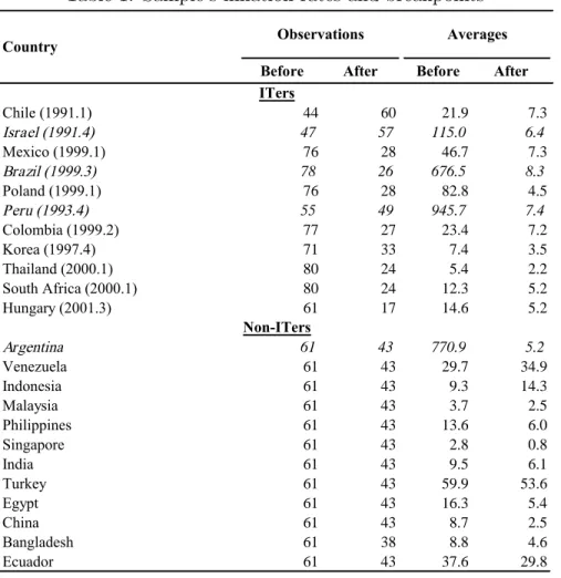
Table 1: Sample’s in‡ation rates and breakpoints
Before After Before After
Chile (1991.1) 44 60 21.9 7.3 Israel (1991.4) 47 57 115.0 6.4 Mexico (1999.1) 76 28 46.7 7.3 Brazil (1999.3) 78 26 676.5 8.3 Poland (1999.1) 76 28 82.8 4.5 Peru (1993.4) 55 49 945.7 7.4 Colombia (1999.2) 77 27 23.4 7.2 Korea (1997.4) 71 33 7.4 3.5 Thailand (2000.1) 80 24 5.4 2.2 South Africa (2000.1) 80 24 12.3 5.2 Hungary (2001.3) 61 17 14.6 5.2 Argentina 61 43 770.9 5.2 Venezuela 61 43 29.7 34.9 Indonesia 61 43 9.3 14.3 Malaysia 61 43 3.7 2.5 Philippines 61 43 13.6 6.0 Singapore 61 43 2.8 0.8 India 61 43 9.5 6.1 Turkey 61 43 59.9 53.6 Egypt 61 43 16.3 5.4 China 61 43 8.7 2.5 Bangladesh 61 38 8.8 4.6 Ecuador 61 43 37.6 29.8
Country Observations Averages
ITers
Non-ITers
we wanted to include the world largest 25 EMEs (measured by the size of their GDP), countries like Russia and Czech Republic lack the minimum information required to be considered in this evaluation.1
Table 1 shows the countries included in the sample and the targeting starting points for our 11 IT countries. For the cross-sectional analysis, the frequency of the data we employ is quarterly. Meanwhile, for the panel analysis the frequency of the information is annual. Data were primarily obtained from the IMF International Financial Statistics (IFS) database.
The sample covers the period between the …rst quarter of 1980 and fourth quarter of 2005. Most of the countries in our sample experienced some degree of de facto exchange rate ‡exibility at some point during this period (Levy-Yeyati and Sturzenegger, 2004). In general, during this lapse, the economies in our sample experimented with a variety
1Other transition economies like Bangladesh and Hungary are included because they initially have at
of monetary and exchange rate regimes that vary from targeting the exchange rate to targeting in‡ation and from pure ‡oating to hard pegs, respectively.2
In a recent paper, Rogo¤ (2003) suggests that one way of illustrating how the recent global disin‡ation has transcended narrow interpretations of monetary regimes is to look at in‡ation performance across di¤erent exchange rate arrangements. As we mentioned above, by employing a sample only containing EMEs, in this paper we deal with a large mix of monetary and exchange rate regimes where NITer countries follow polices which are notably di¤erent to those followed by ITers.
3
In‡ation performance and IT
In this section, we start by assessing IT employing the same Di¤erence-in-Di¤erence model used by BS for a sample of industrial economies. Then, we extend that model to a panel analysis to control for other in‡ation related factors associated with the recent global disin‡ation experience by the world economy.
3.1
Cross-sectional analysis
Using a sample that comprises 20 OECD industrial economies, BS observed that among them the seven economies that adopted IT in the early 1990s were in principle more e¤ective in achieving price stability. However, they noticed that this was explained by the fact that ITers performed signi…cantly worse before adopting the regime. Once they controlled for the so-called “regression to the mean”e¤ect, there was no evidence that IT improves in‡ation performance. In this section, we start by replicating BS estimations for our sample of EMEs.
3.1.1 The model
The Di¤erence-in-Di¤erence (DD) model employed by BS can be derived from a “two-way error component”regression model in which the time series dimension is removed by simply di¤erentiating the average of the data ‘before’and ‘after’a policy change, and then running the underlying di¤erences equation. Starting from a two-way error component
2We see this diversity of regimes as an advantage for our analysis of IT. As mentioned earlier, one of the
critics of Gertler (2003) on Ball and Sheridan’s paper is that, in their sample of 20 OECD countries, NITer countries followed very similar policies to those implemented by the ITers. Under such circumstances, it is then di¢ cult to distinguish the contribution of ITvis-à-vis other regimes.
regression model as described by Baltagi (2001),
it = + xit+uit; i= 1; :::; N; t = 1; :::; T (1)
where i denotes the N countries in the sample and the subscript t denotes time. The dependent variable it is some macroeconomic variable of interest and the error term is
described by uit = i + t +"it, with i representing a country speci…c unobservable
e¤ect, t denoting a time speci…c unobservable e¤ect and"it being the residual stochastic
disturbance.
They contract the panel into only two periods by calculating the average of yit before
and after IT to obtain the pre and post targeting period average levels of ( i;pre and i;post, respectively).3 Then, subtracting the pre average period equation from the post
average period equation we get that
i;post i;pre = ( post pre) + (xi;post xi;pre) + ("i;post "i;pre) (2)
Considering xit, for t =pre or post, to be a dummy variable that takes the value of 1 if
country i targets in‡ation in period t and it is zero otherwise, the DD model is simply reduced to
i;post i;pre = + xi+"i (3)
where i;post i;pre is the e¤ective reduction (or increase) in the average level of , = ( post pre)is the intercept,xi =xi;pre is just a dummy variable that takes the value
of 1 when countryiis targeting in‡ation and"i is the remaining stochastic residual. Most
importantly, the coe¢ cient measures the e¤ect of targeting in‡ation on the behavior of
y, our macroeconomic variable of interest.
Ball and Sheridan (2003) indicate that a problem with this model could arise for some variables of interest if average …gures in the pre-targeting period result substantially di¤erent for targeter and non-targeter economies. This “regression to the mean” e¤ect implies that for some macroeconomic variables (like, for instance, the in‡ation level), the pre-targeting period average might be signi…cantly higher for targeters than non-targeters, thus creating an illusion of greater absolute improvement in the post-targeting period simply because initially the targeters were performing worse than the non-targeters.
To eliminate this regression to the mean bias, they simply propose to include the
3An issue that arises when we split the time into the pre and post-targeting period is the de…nition
of a breakpoint for the control group (i.e. the non-ITer emerging markets). We de…ne several alternative breakpoints which are discussed later on.
pre-targeting average value of y to the model, yi;pre, as an explanatory variable. The
subsequent unbiased model is given by
i;post i;pre= + 1xi+ 2 i;pre+"i (4)
Including i;pre on the right-hand side controls for the regression to the mean bias given
that the coe¢ cient 1 for the dummy variable, if signi…cant, would show the unbiased e¤ect of targeting in‡ation on the dependent variable, for some given initial level of .
3.1.2 Estimations
Table 1 shows in parenthesis the targeting starting points for our 11 IT countries. For non-targeters, the break between the post and pre-targeting period is de…ned as the second quarter of 1995. To de…ne this break point we follow BS and calculate the mid-point quarter between the …rst ITer starting point in the sample (i.e. Chile 1991.1) and the last one (i.e. Hungary 2001.3).
Table 1 also presents the annualized average in‡ation rates for ITers and NITers when the breakpoints for the later group is second quarter of 1995.4 The table shows that our
sample presents considerable cross-country di¤erences in average in‡ation for targeter and non-targeter EMEs, particularly in the pre-targeting period. Among our cross-sectional observations, Brazil, Peru, Israel and Argentina are four extreme cases with average in-‡ation levels in the pre-targeting period that reach three digits.
This problem with outlier observations is frequently faced in analyses of EMEs in‡ation data. In fact, when dealing with in‡ation data, even industrial economies su¤er problems of outliers. In BS, countries that have experienced annual in‡ation rates above 20%, including Greece and Ireland, are excluded from the analysis to avoid such problems.
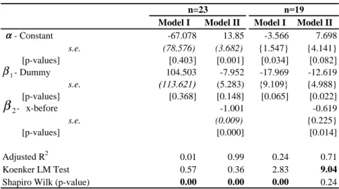
In terms of the estimations, for the IT regime to be contributing toward lower in‡ation, a signi…cant negative coe¢ cient associated to the dummy variable would be expected. Table 2 presents the estimates of the DD model using the two di¤erent speci…cations and two di¤erent data sets. The two speci…cations are the DD model presented in equation (3), which we call Model I, and the adjusted version of the same model to correct for regression to the mean e¤ects, which we call Model II, presented in equation (4). The two data sets comprise the averages of in‡ation with 23 countries (including outliers) and a reduced sample which excludes the four larger outlier countries (i.e. dropping Argentina,
4Notice that Bangladesh and China are omitted from the analysis at this stage because in‡ation data
Table 2: DD model estimates
Model I Model II Model I Model II
- Constant -67.078 13.85 -3.566 7.698 s.e. (78.576) (3.682) {1.547} {4.141} [p-values] [0.403] [0.001] [0.034] [0.082] - Dummy 104.503 -7.952 -17.969 -12.619 s.e. (113.621) (5.283) {9.109} {4.988} [p-values] [0.368] [0.148] [0.065] [0.022] - x-before -1.001 -0.619 s.e. (0.009) {0.225} [p-values] [0.000] [0.014] Adjusted R2 0.01 0.99 0.24 0.71 Koenker LM Test 0.57 0.36 2.83 9.04
Shapiro Wilk (p-value) 0.00 0.00 0.00 0.24
Note: Standard errors in curly brakets {} are heteroskedasticty robust standar errors
n=23 n=19 αα 2
β
α 1 βBrazil, Israel and Peru).
The estimations based on the full sample initially show that the dummy variable capturing the e¤ect of IT on the rate of in‡ation is insigni…cant at the 10% level under both model speci…cations. Correcting for the regression to the mean bias, by including the pre-targeting level of in‡ation in model II, results in a strongly signi…cant regression to the mean e¤ect (p-value 0.000). However, according to the Shapiro–Wilk test, the estimations based on the full sample present problems of non-normality.5 Since this problem is likely
to be encountered in the presence of outliers, we drop from the sample the four countries with the largest in‡ation averages in the pre-targeting period (i.e. Argentina, Brazil, Israel and Peru). Estimations based on the reduced sample turn out to show a signi…cant IT dummy coe¢ cient at the 5% level and appear to be free from normality problems once that the model control for regression to the mean e¤ect.
Other estimations where we drop the …rst half of the 1980s or where we employ alternative intermediate breakpoints (e.g. 1993.3 as in BS) provided similar results6.
Overall, once we control for outlier observations, our results reveal that the EMEs that adopted IT have performed better than the non-targeters in terms of in‡ation. This result clearly contrasts with Ball and Sheridan’s (2003) conclusion with respect to the e¤ect of IT on average in‡ation levels for their sample of industrial economies.
5Because of our small cross-sectional sample,t-tests are not asymptotically valid under non-normality. 6We chose 1990.1 by calculating for each country in the sample the …ve quarter moving average
in‡ation rate, then the average across the sample and observing this period as a clear trend change in the average in‡ation level.
3.2
Panel analysis
In this section we re-introduce the time dimension of our sample to explore whether a panel analysis, which considers other in‡ation determinants, provides evidence to support the results we found using the cross-sectional analysis. In addition to introducing variables commonly associated with in‡ation performance, like the government primary surplus, GDP growth and worldwide shock variables, we control for the in‡uence of other less traditional factors that the literature has associated with recent disin‡ation. In particular, we incorporate the impact of two other factors suggested by Rogo¤ (2003) as determinants of worldwide disin‡ation: globalization and prudent …scal policies.
3.2.1 The model
The speci…cation of the model departs from equation (1) where, in addition to modelling the behavior of in‡ation as a function a dummy variable Tit, we control for the e¤ect of
country speci…c factors and world shocks. More precisely, the rate of in‡ation observed in each period t and for each country i; i;t, is modelled as
i;t = + Tit+ 1git+ 2 yit 1+ 3Iit+ 1Ptoil + 2 yust +uit (5)
where git is the government primary surplus as a proportion of GDP, yit 1 is the …rst
lag of GDP growth, Iit is our proxy for globalization and it is equal to total trade in
goods divided by GDP and the variable Poil
t and yust are shock variables that represent,
respectively, the change in the price of oil and the growth rate of output for the US economy.7 We expect the …rst lag of GDP growth to have an increasing e¤ect over the rate of in‡ation at periodt; while the government primary surplus and trade integration (our proxy for globalization) to have a reducing e¤ect. Oil prices and the state of the world economy (measured by rate of growth of the US economy), both variables are expected to have a positive impact on in‡ation.
3.2.2 Estimations
In order to avoid normality problems, for the panel estimations we drop the three largest in‡ation outlier countries from our sample (Argentina, Brazil, Israel and Peru). Due to
7According to Sumner (2004), it is largely accepted that contemporary globalization is de…ned by
global economic integration in terms of current and capital accounts. Since trade in goods and services has been suggested as a signi…cant factor contributing towards global disin‡ation (Rogo¤, 2003), the estimations presented here focus on examining the in‡uence of trade ‡ows (and increasing competition) on price stability.
Table 3: Aggregate e¤ect of in‡ation targeting Variables OLS* GLS Constant (∪i) 18.321 12.834 [0.074] [0.000] IT dummy (Tit) -12.362 -6.236 [0.000] [0.000] Government primary surplus (git) -2.395 -0.608 [0.012] [0.000] Lag of GDP growth (yit-1) -0.465 0.118
[0.157] [0.000] World trade integration (Iwt) -1.263 -4.689 [0.671] [0.000] Change in oil price (Pt
oil
) -0.140 0.151
[0.522] [0.069]
US GDP growth (yusit) 1.034 0.473
[0.454] [0.016]
* P-values in square brackets calcualted using Newey-West standar errors
several missing observations concerning country-speci…c factors we also exclude Poland, Hungary and Bangladesh from the analysis. In addition, because of some of the country speci…c factors are not yet available for 2005, the time span of the sample is reduced to 2004.
In sum, we observe the behavior of in‡ation on a sample comprising 6 ITers and 10 non-ITers during 25 years for a total of 400 observations. As with the DD model, our main source of data is the International Financial Statistics database from the IMF.
We start by estimating (5) by OLS, pooling time series and cross section observations. Tests of heteroscedasticity and autocorrelation reveal that both problems coexist in the initial estimations. Therefore, we re-estimate the model and report Newey–West standard errors, which are robust to heteroscedasticity and …rst-degree autocorrelation. Following these estimations, the results in Table 3 show that the IT dummy that captures the aggregate e¤ect of IT is negative and signi…cant at the 1% level. The government primary surplus, which controls for the e¤ect of prudent …scal policies on the reduction of in‡ation, also presents the expected sign and is signi…cant at the 5% level. The ratio of total trade (i.e. import plus exports) to output, our proxy for globalization, presents the negative expected sign but it is insigni…cant at the 10% level. The …rst lag of GDP is the only country speci…c variable in the model that is not just insigni…cant but also presents the unanticipated sign. Finally, the coe¢ cients for those variables included in the model to capture the e¤ect of world shocks, US GDP growth and oil prices, both are clearly insigni…cant.
As an alternative to OLS, we estimate (5) as a system of equations through GLS. The advantage of this approach is that instead of relying on robust standard errors we can allow the disturbances to have a heteroscedastic and at the same time autocorrelated structure. Moreover, given the characteristics of our data, we can allow the residuals to be cross-sectionally correlated. We would expect that in a globally integrated …nancial environment like the one confronted by EMEs— where propagation of shocks through contagion spread from one country to another— residuals would be contemporaneously correlated.
In order to test for contemporaneous correlation of the residuals, we use the errors ob-tained from the OLS estimations to compute the Breusch–Pagan LM test of cross-sectional independence. The null hypothesis of this test is that all countries are independent of each other, while under the alternative hypothesis the residuals of at least two of the countries in the sample are contemporaneously correlated. The resulting test statistic is distributed as a 2 with N(N 1)=2degrees of freedom (see Greene, 2000). The value of
the Breusch–Pagan statistic is344:01> 2
0:99(120) = 159; which clearly suggests that the
null has to be rejected.
In summary, the system of regression equations estimated through GLS present the following characteristics:
E("it; "it) = 2i (6)
E("it; "it 1) = i (7)
E("it; "jt) = 2ij (8)
where (6) suggests that the residual are heteroscedastic, (7) that are autocorrelated and (8) that they are cross-sectionally correlated.
Table 3 also presents the results for the estimation of the model as a system of equations through GLS. Allowing for cross-sectional correlation improves the signi…cance of most of the coe¢ cients of the model. The IT dummy remains signi…cant at the 1% level. In fact, all the other country speci…c variables of the model become signi…cant at the 1% level and present the expected sign, including the coe¢ cients for the lag of GDP and world trade, which were not signi…cant, and in the case of the former presented the wrong sign, when estimated by OLS. The only variables that are not signi…cant at the 1% level following the estimation through GLS are the shock variables: US GDP growth and oil prices; however, they are both signi…cant at the 10% and 5% level respectively. Overall, the panel analysis con…rms the results found through the cross-sectional estimations, even accounting for other disin‡ation related factors, IT has matter for EMEs price stability.
4
Conclusion
This paper has attempted to investigate the e¤ect of IT on price stability employing a sample comprised by EMEs. Our …ndings clearly contrast with those of Ball and Sheridan (2003) for their sample of industrial economies. Cross-section and panel estimations consistently suggest that IT has mattered for EMEs disin‡ation. Controlling for other relevant disin‡ation related factors only con…rms the in‡uence of IT on price stability.
We conclude that IT really mattered for EMEs disin‡ation. Nevertheless, there is no reason to believe that this would not change in the future. For emerging and industrial economies, the experience with IT has been analyzed mainly under periods of relative macroeconomic stability. Little is known about the properties of this regime for periods of instability. Certainly, the attributes of the regime under periods of macroeconomic distress must be of great concern for EMEs.
References
[1] Baltagi, B. H. (2001). Econometric Analysis of Panel Data, John Wiley and Sons, Chichester.
[2] Ball, L. and Sheridan, N. (2003). “Does In‡ation Targeting Matters?”, NBER Macro-economics Annual 2003, Volume 18.
[3] Gertler, M. (2003). “Comment on Ball, L. and Sheridan, N., "Does In‡ation Target-ing Matters?",”, NBER Macroeconomics Annual 2003, Volume 18.
[4] Greene W. H. (2002). "Econometric Analysis", Fourth Edition, Prentice Hall Inter-national Ltd., London, UK.
[5] Johnson, D. (2002). “The E¤ect of In‡ation Targeting on the Behavior of Expected In‡ation: Evidence from a 11 Country Panel”, Journal of Monetary Economics 49(8), p. 1521-1538.
[6] Levy-Yeyati, E. and Sturzenegger, F. (2005). “Classifying Exchange Rate Regimes: Deeds and Words”, forthcoming European Economic Review.
[7] Mishkin, F. (2002). “Comments on Newman, M. J. and von Hagen. J. "Does In‡ation Targeting Matter?",” , Review Federal Reserve Bank of San Luis 84(4), p. 149-153.
[8] Newman, M. J. and von Hagen, J. (2002). “Does In‡ation Targeting Matters?”, Review Federal Reserve Bank of San Luis 84 (4), p. 127-148.
[9] Rogo¤, K. S. (2003). “Globalization and Global Disin‡ation”, Paper prepared for the Federal Reserve Bank of Kansas City conference on ‘Monetary Policy and Un-certainty: Adapting to a Changing Economy’Jackson Hole, WY, available online at http://www.imf.org/external/np/speeches/2003/082903.htm.
[10] Sumner, A. (2004). “Why are We Still Arguing about Globalization”, Journal of International Development 16 (7), p. 1015-1122.
[11] Uhlig, H. (2004). “Commentary on Levin, A. Natalucci, F. M. and Piger, J. M., "The Macroeconomic E¤ects of In‡ation Targeting",”, Federal Reserve Bank of St. Louis Review 86 (4), p. 81-88.