Three Papers on the Black-White Mobility Gap in the United States

Three Papers on the Black-White Mobility Gap in the United States

Liana E. Fox

Submitted in partial fulfillment of the requirements for the degree of

Doctor of Philosophy under the Executive Committee of the Graduate School of Arts and Sciences

COLUMBIA UNIVERSITY 2013

© 2013 Liana E. Fox All rights reserved

A

Three Papers on the Black-White Mobility Gap in the United States Liana E. Fox

Paper 1/Chapter 2: Missing at Random? An Analysis of the Effect of Sample Selection on Intergenerational Earnings Elasticities by Race

Utilizing the Panel Study of Income Dynamics, I assess the effect of sample selection bias on estimates of intergenerational earnings elasticities for white and black father-son pairs, regressing log child earnings on log parent earnings. Estimating four increasingly less selected models, I assess the robustness of estimates to alternative methods of handling sons who are missing data due to periods of unemployment or part-time employment. The results indicate that the assumption of exogenous selection into full-time employment significantly biases the

estimates for blacks, although it does not have a large impact on estimates for whites. As a consequence, selection bias will understate the magnitude of the black-white mobility gap. The results also indicate that two methods substantially mitigate this selection bias: having a long panel, or imputing data in a short panel.

Paper 2/Chapter 3: Measuring the Black-White Mobility Gap: A Comparison of Datasets and Methods

Chapter 3 utilizes both the National Longitudinal Survey of Youth (NLSY) and the Panel Study of Income Dynamics (PSID) to analyze the magnitude and nature of black-white gaps in intergenerational earnings and income mobility in the United States. This chapter finds that relying on different datasets or measures will lead to different conclusions about the relative magnitudes of black versus white elasticities and correlations, but using directional mobility matrices consistently reveals a sizable mobility gap between black and white families, with

low-income black families disproportionately trapped at the bottom of the low-income distribution and more advantaged black children more likely to lose that advantage in adulthood than similarly situated white children. I find the family income analyses to be most consistent and estimate the upward mobility gap as between 19.1 and 20.3 percentage points and the downward gap between -20.9 and -21.0. Additionally, I find that racial disparities are much greater among sons than daughters and that incarceration and being raised in a female-headed household have much larger impacts on the mobility prospects of blacks than whites.

Paper 3/Chapter 4: Can Parental Wealth Explain the Black-White Mobility Gap?

Utilizing longitudinal data from the Panel Study of Income Dynamics (PSID), this

chapter examines the relationship between parental wealth and intergenerational income mobility for black and white families. I find that total parental wealth promotes upward mobility for low-income white families, but does not protect against downward mobility for white families from the top half of the income distribution. Conversely, I find that total parental wealth does not assist low-income black families while home ownership may have negative associations with the likelihood of upward mobility for these families. However, for black families from the top half of the income distribution home equity is protective against downward mobility suggesting a heterogeneous relationship between home ownership and mobility for black families.

i

T

C

LIST OF TABLES AND FIGURES ... ii

ACKNOWLEDGMENTS ... vi

DEDICATION ... viii

CHAPTER 1:INTRODUCTION ... 1

CHAPTER 2:MISSING AT RANDOM?AN ANALYSIS OF THE EFFECT OF SAMPLE SELECTION ON INTERGENERATIONAL EARNINGS ELASTICITIES BY RACE ... 3

CHAPTER 3:MEASURING THE BLACK-WHITE MOBILITY GAP:A COMPARISON OF DATASETS AND METHODS ... 27

CHAPTER 4:CAN PARENTAL WEALTH EXPLAIN THE BLACK-WHITE MOBILITY GAP? ... 79

ii

L

T

F

Table 2.1: Intergenerational Elasticities, by Model Specification and Race….……..……….22

Table 2.2: First-Stage Imputed Earnings Results, ̂ ………..………..……23

Table 2.3: Comparison of Intergenerational Elasticities by Actual vs. Imputed Earnings and Race………..……….……….24

Figure 2.1.A: Only FT (N=444)………25

Figure 2.1.B: Lower-Bound (N=757)…..…….……….25

Figure 2.1.C: Upper-Bound (N=757)…...……….25

Appendix Table 2.1: Average Earnings, by model specification and race………26

Table 3.1: Descriptive Statistics for NLSY v PSID Samples…...………..……….54

Table 3.2: Intergenerational Elasticities and Correlations PSID v NLSY………55

Table 3.3: Likelihood of Upward and Downward Mobility by Race, NLSY and PSID………...56

Appendix Table 3.1: Intergenerational Elasticities and Correlations by Incarceration History, Overall………..……….57

Appendix Table 3.2: Intergenerational Elasticities and Correlations by Incarceration History, White, non-Hispanic Families………..……….58

Appendix Table 3.3: Intergenerational Elasticities and Correlations by Incarceration History, Black, non-Hispanic Families………..……….59

Appendix Table 3.4: Intergenerational Elasticities and Correlations by Family Structure, Overall………..…….60

Appendix Table 3.5: Intergenerational Elasticities and Correlations by Family Structure, White, non-Hispanic Families……..……….61

Appendix Table 3.6: Intergenerational Elasticities and Correlations by Family Structure, Black, non-Hispanic Families………..……….62

Appendix Table 3.7: Likelihood of Upward and Downward Mobility by Race for Never-Incarcerated Population, NLSY and PSID………63

Appendix Table 3.8: NLSY Family Income-Family Income Mobility Matrices by Race (Sons & Daughters)……….…64

iii

Appendix Table 3.9: NLSY Family Income-Family Income Mobility Matrices by Race (Sons)……….…65 Appendix Table 3.10: NLSY Family Income-Family Income Mobility Matrices by Race (Daughters)...……….…66 Appendix Table 3.11: NLSY Family Income-Child Earnings Mobility Matrices by Race (Sons & Daughters)…..……….…67 Appendix Table 3.12: NLSY Family Income- Child Earnings Mobility Matrices by Race (Sons)……….…68 Appendix Table 3.13: NLSY Family Income- Child Earnings Mobility Matrices by Race (Daughters)...……….…69 Appendix Table 3.14: PSID #3 Family Income-Family Income Mobility Matrices by Race (Sons & Daughters)………..……….…70 Appendix Table 3.15: PSID #3 Family Income-Family Income Mobility Matrices by Race (Sons)……….…71 Appendix Table 3.16: PSID #3 Family Income-Family Income Mobility Matrices by Race (Daughters)...……….…72 Appendix Table 3.17: PSID #3 Family Income-Child Earnings Mobility Matrices by Race (Sons & Daughters)………..……….…73 Appendix Table 3.18: PSID #3 Family Income-Child Earnings Mobility Matrices by Race (Sons)……….…74 Appendix Table 3.19: PSID #3 Family Income-Child Earnings Mobility Matrices by Race (Daughters)...……….…75 Appendix Table 3.20: PSID #3 Father Earnings-Child Earnings Mobility Matrices by Race (Sons & Daughters)………..……….…76 Appendix Table 3.21: PSID #3 Father Earnings-Child Earnings Mobility Matrices by Race (Sons)……….…77 Appendix Table 3.22: PSID #3 Father Earnings-Child Earnings Mobility Matrices by Race (Daughters)...……….…78 Figure 4.1: Median Family Net Worth, 1984-2009 (in 2009$)……….……….99 Figure 4.2: Median Family Net Worth Excluding Home Equity, 1984-2009 (in 2009$)………...99

iv

Figure 4.3: Distribution of White Families by Net Worth, 1984-2009………....100

Figure 4.4: Distribution of Black Families by Net Worth, 1984-2009……….…100

Figure 4.5: Median Net Worth by Race and Head Education, 1984-2009………..101

Figure 4.6: Distribution of Parent Generation………....102

Figure 4.7: Distribution of Child Generation………..………....102

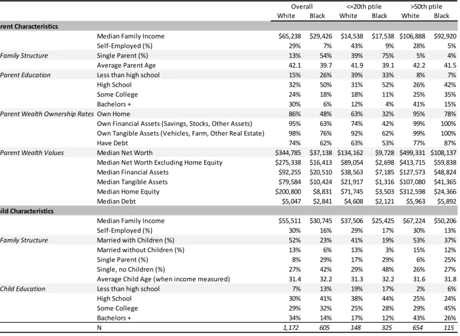
Table 4.1: Demographic Characteristics of Sample by Race and Parental Ranking…….…….103

Table 4.2: Parental Wealth Holdings by Asset Type and Race, 1984-2009 (2009$)…………..104

Table 4.3a: Likelihood of Upward Mobility by Race………...105

Figure 4.8: Upward Mobility by Race, Parent Rank<=20………..106

Figure 4.9: W-B Upward Mobility Gap………..……….106

Table 4.3b: Likelihood of Downward Mobility by Race………..107

Figure 4.10: Downward Mobility by Race, Parent Rank>50………..108

Figure 4.11: W-B Downward Mobility Gap……….108

Table 4.4a: Likelihood of Upward Mobility from Bottom 20%, Conditional on Parental Wealth Attributes……...………...109

Table 4.4b: Likelihood of Downward Mobility from Top 50%, Conditional on Parental Wealth Attributes……...………...109

Table 4.5: Likelihood of Mobility by Asset Values and Race………..110

Table 4.6: Real Home Equity (low income home owners in 1984)………..111

Table 4.7: Decomposition of the Effects of Wealth on White-Black Upward Mobility Gap…...112

Appendix Figure 4.1: Percentiles of Net Worth for White Families, 1984-2009………113

Appendix Figure 4.2: Percentiles of Net Worth for Black Families, 1984-2009………113

Appendix Table 4.1a: Likelihood of Upward Mobility by Race—Adjusted by Family Size……114

Appendix Table 4.1b: Likelihood of Downward Mobility by Race……….114

Appendix Table 4.2a: Likelihood of Upward Mobility by Race—Adjusted by Family Size……115

v

Appendix Table 4.3a: Likelihood of Upward Mobility by Race—Adjusted by Family Size……116 Appendix Table 4.3b: Likelihood of Downward Mobility by Race……….116 Appendix Table 4.4: Decomposition of Wealth on Upward Mobility……….117

vi

A

Over the past four and a half years I have received support and encouragement from a great number of individuals. First and foremost I would like to express my deepest gratitude to my advisor, Jane Waldfogel, for her never-ending encouragement, guidance and providing me with an excellent atmosphere for doing research. I owe sincere and earnest thankfulness to my sponsor, Irwin Garfinkel, who has continually challenged and enriched my understanding of social welfare policy. I am also very thankful to the rest of my dissertation committee of Ronald Mincy, Seymour Spilerman and Judith Scott-Clayton for providing me with advice and

encouragement through coursework and individual meetings as my interests have developed. I would like to express my gratitude to my classmates Nathan Hutto and Leyla Karimli for their generous friendships and solidarity. Thanks to Natasha Pilkauskas and Afshin

Zilanawala for answering my streams of questions and providing much needed breaks throughout this process. I would also like to thank my previous advisors and mentors: Kate Bronfenbrenner who helped channel my social justice consciousness, Stephanie Luce who helped me gain a deeper understanding of the power of empirical research, Mark Brenner who patiently spent hours teaching me SAS, and Michael Ettlinger who introduced me to the world of policy analysis.

Finally, I would like to thank my family, both immediate and extended, for their encouragement and support. I thank my daughter Hazel for teaching me a new level of time management and multitasking. Not the least, I appreciate the personal and financial sacrifices made by my husband Chris which allowed me to pursue this degree. Thank you for being my teammate.

vii

This research was supported by the Columbia Population Research Center (award number R24HD058486 from the Eunice Kennedy Shriver National Institute of Child Health & Human Development) for travel support to present Chapters 2 and 4 at the Population

Association of America’s Annual Meetings. Research for Chapter 4 was also supported by a grant from the Pew Charitable Trusts and Charles Stewart Mott Foundations. Opinions reflect those of the author and do not necessarily reflect those of the granting agencies.

viii

D

1

C

1:

I

The United States is often described as the land of opportunity. However, with the dramatic increase in income inequality since the 1970s, the equality of this opportunity has been called into question. As a society, we are willing to tolerate inequality as long as there is fairness and opportunity for all individuals to succeed, regardless of family background. However, recent analyses (Hertz 2007; Isaacs 2008) find that opportunity may not apply equally to all citizens. While the black-white male wage gap has closed considerably since passage of the Civil Rights Act of 1964, black families are more likely to remain poor and experience relative (and often absolute) declines in income position from one generation to the next compared with white families. From a social welfare perspective, this means that an extra dollar of income does not guarantee the same level of long-run economic success for black families as white families. Research focusing on black-white economic disparities has found a narrowing of the male wage gap from 50% in 1967 to 27% in 1998 (Couch and Daly 2002), while the family income gap has closed considerably less, with median black family income comprising 59% of the median white family income in 1967 and 62% in 2007 (Mishel, Bernstein and Shierholz 2009). These

comparisons highlight the importance of examining both individual earnings and family income to get a complete portrait of relative economic well-being and opportunity.

One measure of opportunity in society is intergenerational mobility, which can be measured by examining the relationship between children’s income or earnings with respect to the same measure for their parents. This relationship can be quantified by estimating the elasticity or correlation or by predicting the likelihood of directional mobility between two generations. Higher elasticities indicate greater similarity between outcomes for children and parents and therefore lower mobility. While conceptually the most complete measure of

2

intergenerational transmission of economic well-being would be the comparison of parental family income to child family income, it also conflates trends and disparities in employment and family structure. However, examining only earnings results in a selected sample that may not be representative of the total population. Therefore, deciding when to examine intergenerational persistence in family income versus individual earnings represents a tradeoff between a more inclusive measure and population and a better-defined mechanism structure. This dissertation explores several methodological issues in estimating the magnitude of these disparities, as well as examines the role of wealth in explaining the black-white mobility gap.

Chapter 2 utilizes the Panel Study of Income Dynamics (PSID) to provide new estimates of intergenerational earnings elasticities for white and black father-son pairs estimated using the traditional methodology of regressing log child earnings on log parent earnings. This chapter pays special attention to the impact of sample selection (i.e. excluding unemployed or part-time employed sons from the sample) on intergenerational mobility estimates. I generate predicted estimates of son’s potential earnings (as actual earnings have been censored due to either

unemployment or underemployment) and then perform a bounding exercise to examine the range of estimates.

Chapter 3 expands on Chapter 2 by comprehensively examining family income mobility in addition to earnings mobility. The more inclusive measure of family income extends the previous analysis of father-son earnings to include all sources of economic well-being and also allows for the examination of individuals from otherwise excluded family structures such as female-headed households. This chapter utilizes both the National Longitudinal Survey of Youth (NLSY) and the Panel Study on Income Dynamics (PSID) datasets as well as multiple methods of estimating intergenerational mobility (elasticities, correlations and directional rank matrices)

3

to quantify the magnitude and nature of the black-white family income mobility gap in the United States. It also tests the sensitivity of results to incarceration and family structure.

Chapter 4 builds off of methodological advances discussed in the previous two chapters in an effort to explain the mobility gap by examining the relationship between parental wealth and intergenerational income mobility for black and white families. Utilizing the PSID Wealth Supplements, I estimate how parental wealth impacts children’s directional income mobility for black and white families and explore differences in this impact by asset type. I also perform a decomposition analysis to investigate the role of wealth/capital accumulation in explaining the economic mobility gap.

Finally, Chapter 5 provides a summary of the main results from Chapters 2-4 and discusses implications for policy and social work practice. While the individual chapters cover slightly different years and cohorts, with parental resources measured in 1968-82 in Chapter 2, 1979-81 in Chapter 3 and 1984-89 in Chapter 4, and child resources measured in 1997-2009 in each chapter, an attempt is made to compare results across chapters. Areas of future research are also highlighted.

REFERENCES

Couch, K. and M. C. Daly. (2002). ―Black-white wage inequality in the 1990s: A decade of progress.‖ Economic Inquiry. 40(1):31-41.

Hertz, T. (2007). ―Trends in the intergenerational elasticity of family income in the United States.‖ Industrial Relations. 46(1): 22-50.

Isaacs, J.B. (2008). ―Economic Mobility of Black and White Families.‖ In Isaacs, J.B. Sawhill, I. and Haskins, R. Getting ahead or losing ground: economic mobility in America.

(Washington D.C.: Brookings Institute). pp71-80.

Mishel, L., J. Bernstein and H. Shierholz. (2009). The State of Working America, 2008/2009. Ithaca, NY: ILR Press, an imprint of Cornell University Press.

4

C

2:

M

R

?

A

SELECTION ON INTERGENERATIONAL EARNINGS ELASTICITIES BY RACE

INTRODUCTION

Intergenerational mobility is an important measure of social equality and opportunity in a country. Higher mobility signals more potential for individuals to prosper or fail based on

individual effort or attributes, while lower mobility signals a system where status is primarily based on family background. Economists and sociologists have been attempting to measure intergenerational mobility for decades, but new methods continue to challenge previous findings (Solon 1999; Black & Devereux 2010). Previous research has highlighted the importance of using permanent income measures rather than single-year income measures (Grawe 2006; Haider & Solon 2006). Similarly, due to life-cycle variation in income, the age at which income is observed matters quite a bit, and ideally should be measured from both generations while they are in their 30s-40s (Solon 1999; Black & Devereux 2010) and age-adjusted to account for age differences within a sample (Solon 1992; Bratberg et al 2007). Additionally, more recent work has focused on non-linearities in mobility, with both the lowest and highest income families experiencing a greater deal of ―stickiness‖ than do middle income families (Hertz 2005; Grawe 2004; Eide & Showalter 1999).

While all these potential sources of bias have been corrected for in recent research, there still exists one potentially serious concern: sample selection bias. Typically, intergenerational mobility is measured by estimating the elasticity between parents’ income or earnings and the same measure for their children. Higher elasticities (i.e. closer to 1) indicate greater reliance on parents’ income and therefore lower mobility (the direction of mobility—upward or

5

intergenerational elasticity it is common to exclude unemployed and part-time employed

children (or individuals who report no income or earnings) from the sample with the assumption of exogenous selection into full-time employment. However, evidence suggests that sons from lower income families may have a weaker attachment to the labor force and therefore lower mobility, so excluding individuals with perhaps the highest elasticities introduces a downward bias to the current intergenerational elasticity estimates. A few papers have examined selection bias in the intergenerational mobility literature and found it to be a problem (Couch & Lillard 1998; Minicozzi 2003; Francesconi & Nicoletti 2006). However, this literature has not examined the effect of selection bias on estimates of how mobility differs by race. This is a potentially serious omission given that the extent of bias associated with missing employment data is likely to be much more severe for blacks than for whites, given their lower adult employment rates.

This chapter therefore provides new estimates of intergenerational elasticities for blacks and whites explicitly taking into account the effect of selection bias. To that end, I examine the impact of four alternative approaches to missing data on sons’ earnings. The first model follows the standard assumption of ―exogenous‖ selection into full-time employment, restricting the sample to sons who were employed full-time at age 35/36 and 37/38. The second model reduces missing data by imputing a predicted value of sons’ earnings for individuals with earnings

censored by part-time employment or unemployment. The third model also reduces missing data by utilizing upper and lower bounds on sons’ earnings that have been censored by part-time employment or unemployment to estimate the range of potential elasticities. Finally, the fourth model is the most inclusive, allowing information on sons’ earnings from full-time employment to be drawn from 20 years of data (from son’s age 35-55), a specification that would only

6

exclude individuals who dropped out of the PSID or who were consistently unemployed or part-time employed for their entire prime-age working careers.

BACKGROUND

In attempting to explain the differences in intergenerational mobility estimates in the literature, several papers have examined the impact of sample selection bias. First, Couch and Lillard (1998) found that intergenerational correlations are very sensitive to selection rules. They found that a more restrictive sample, which was often more homogenous, led to higher

intergenerational income correlations. Specifically the authors warn against excluding estimates of low-earnings (even if due to part-time employment or unemployment); stating that such exclusions should only be done if one is trying to explicitly identify a sub-population, not examine overall mobility rates.

However, in 2003, Minicozzi found the opposite result—excluding part-time and unemployed workers biased the intergenerational elasticities downward. Minicozzi found that differential treatment of part-time employed workers accounts for some of the variation in estimates across current studies. While the exact reasons for the disparities in findings between Couch and Lillard and Minicozzi are not readily apparent, Minicozzi had a larger sample size and focused on sons aged 27-29, while Couch and Lillard had a wider age range (22-30). Studies that estimate elasticities at younger ages tend to produce smaller estimates (Solon 1999), but that would suggest that Couch and Lillard’s estimates should be lower than Minicozzi’s which was not the case.

In 2006, Francesconi and Nicoletti set aside earlier findings on sample selection and focused on non-labor market selection processes such as ―non-ignorable attrition‖ and short panels. They found evidence of co-residence bias, which means that children who co-reside with

7

their parents at late ages will have better measures of initial status due to more years of measured parental income. The authors find evidence of a downward bias in intergenerational elasticities, especially at the ends of the occupational prestige distribution (used instead of earnings/income to avoid labor market selection issues). This bias is especially problematic in short panels. Taken together, these three papers highlight the importance of sample selection, although the ultimate direction of bias is unclear.

DATA

For this analysis, I use the Panel Study on Income Dynamics (PSID), which is a

longitudinal survey that follows individuals and their offspring from 1968 to present. The survey was conducted annually from 1968-1997 and biannually since then, with the most recent data covering 2007. The PSID includes rich data on labor earnings, hours worked, employment status and family relationships. Using this data it is possible to identify individuals whose earnings have been censored by working part-time or part-year, but unfortunately it is not possible to tell whether individuals are voluntarily choosing to work part-time, or whether this type of

employment is due to economic conditions restricting their opportunities. Sample Restrictions

As one of the main goals of this analysis is to examine the effect of sample selection on intergenerational elasticity measures, I am very deliberate about selecting my own sample. Since the issue of selection becomes much less clear when thinking about women opting out of the labor force to raise children, I focus my analysis on the relationship between sons and their fathers. 1 As a very high percent of prime-age men work full-time, it is not a stretch to assume

1

Implicit in this framework is that I am only looking at sons raised in male-headed families since I am looking at the relationship between father and son earnings. I choose this restriction so as to focus on issues related to

intergenerational earnings transmissions and not to confuse the issue of family structure. A preliminary analysis suggests that individuals raised in female-headed families have considerably lower income elasticities (i.e. sons’

8

that most prime-age men would work full-time if they had the opportunity, which theoretically allows the assumption of exogenous selection into full-time employment to have some validity. My overall sample is restricted to white and black father-son pairs in the PSID with at least three years of valid father earnings while the son was living at home under 21 years old and the father was between age 35-55. 2 As a result of these restrictions, the father cohort was born between 1904-1938 and the son cohort was born between 1954-1973. Further restrictions for each model are detailed below.

Earnings in the PSID include the individual’s annual earnings from labor including salaries, wages, bonuses, overtime, and commissions. For this analysis, earnings are first adjusted to 2006 dollars using the CPI-U, logged and then averaged for all available years. Father’s earnings are only included for years when the son lived at home and was age 21 or below and the father was between 35 and 55 years old. Sons’ earnings are included for years when the son lived outside of his parents’ home and was employed full-time (>2,000 hours/year). METHODS

Following the standard intergenerational mobility methodology (Black & Devereux 2010), I calculate the intergenerational earnings elasticity by regressing the log of permanent child earnings on the log of permanent parent earnings:

( ) (1)

earnings are much less related to parents’ earnings) than individuals raised in a two-parent family (0.11 vs. 0.36 elasticity). This assumption is especially important when looking at families by race, as a very rough examination of a single year of PSID data shows that 37% of black sons lived in a female-headed family compared with 11% of white sons. However, family structure is volatile, so many of these individuals are included in the final sample in years when their father (or other cohabiting adult male) is present. Chapter 3 explores relaxing this restriction. 2 _{Findings are robust to choice of restriction on fathers’ ages, whether they are restricted to age 35-55 or 30-60. Age} range of 35-55 was used in this analysis to be consistent with recommendations from Haider and Solon (2006) and the age restriction used in Model 4.

9

Consistent with current methodology (Black & Devereux 2010), I estimate Equation 1 by first subtracting the mean value of log earnings from each observation to suppress the constant term (Equation 1a) and then age-adjust son and parent earnings to account for life-cycle variation in earnings (Equations 1b & 1c).3

( ( ̅̅̅̅̅̅̅̅̅̅̅̅̅̅̅) ) ( ) ̅̅̅̅̅̅̅̅̅̅̅̅̅̅̅̅̅ (1a)

To age-adjust earnings, I follow previous research (Bratberg et al 2007) and regress log earnings on age and age-squared and use the residual in the final estimation equation:

( ) ( ) (1b) ( ) ( ) (1c) This results in the following simplified equation:

(2) where is the intergenerational earnings elasticity, lower-case is the age-adjusted,

de-meaned value of log earnings and is the error term. The interpretation of is that the closer it is to 1, the less mobility in society, as a large percent of variation in a son’s earnings comes from his father’s earnings, while the closer is to 0, the greater the mobility.4

This is the method used for calculating intergenerational elasticities in all of my models, although the procedure for estimating and selecting sons into the sample varies from model to model. For each model I estimate an overall elasticity, a white elasticity and a black elasticity. I start from the most restrictive model and expand out, investigating alternative

methodologies for estimating permanent child earnings which allow for the inclusion of a greater

3 _{Mean values of both son and father earnings can be found in Appendix Table 2.1.}

4 _{There is a great deal of debate on the ―optimal‖ level of mobility in society (see Bowles, Gintis & Osborne Groves} 2005).

10

number of father-son pairs into the sample, which should therefore allow for greater representativeness and generalizability of results.

Model 1: “Exogenous” selection into full-time employment

In my first model, I restrict the sample to sons who were employed full-time at both age 35/36 and age 37/38 (N=444). This model best estimates the current methodology in the

literature, which assumes that sons are exogenously selected into full-time employment. This is the most restrictive model as no information from sons who are employed part-time or

unemployed is included in this estimation of intergenerational elasticity. Additionally,

individuals with missing earnings data during either of these two time periods are excluded. In this specification I am drawing on 2 years of sons’ earnings and an average of 9.7 years of fathers’ earnings information. Average earnings can be found in Appendix Table 2.1 for each model specification both overall and by race.

Model 2: Imputed earnings at age 35/36 and 37/38 for part-time/unemployed sons

To examine the role of ―exogenous‖ selection, I estimate an imputed value of son’s potential earnings as a proxy for actual labor earnings.5 Potential earnings at age 35/36 and 37/38 are estimated from the average earnings from full-time employment while age 25-34 and age 39-55 as well as a range of demographic characteristics. In my imputation the first-stage equation is:

̂ ̅ (3)

5 _{Alternatively, in lieu of this imputation procedure, I could have used earnings from sons in their twenties and used} an adjustment factor to scale up these values, but I was hesitant to use such an adjustment factor due to differences in life-cycle growth of wages. According to Haider and Solon (2006), using earnings from an individual in their twenties causes a large attenuation bias, but the bias is small if earnings are measured between the early thirties and the mid-forties. Additionally, Haider and Solon found that individuals with the greatest potential lifetime earnings often have lower earnings than other individuals early on in their careers as this time is often spent in education or taking risks (i.e. starting a business) with larger potential payouts in the future. To avoid this life-cycle bias, I chose to impute earnings values based on average actual earnings at both younger and older ages, as well as other human capital components such as education and marital status.

11 where ̅ is average earnings from full-time employment at age 25-34 and age 39-55 and is a vector of individual characteristics (educational attainment, race, age, age-squared, marital status, and state of residence). The results from this first-stage equation are displayed in Table 2.2. From this equation, I then generate predicted values of ̂ for all sons and plug those values into equation 2.

Therefore, my second-stage equation is:

̂ (4)

where is the intergenerational earnings elasticity adjusted for selection with the same interpretation as the earlier elasticity. For consistency, all sons are given imputed values for ̂ even if they had valid earnings information for those years. An examination of this imputation process can be found in Table 2.3, which compares imputed earnings to actual

earnings. By imputing values of sons’ earnings for unemployed and part-time employed sons, the sample size for this model increases to 757. In this specification I utilize an average of 4.5 years of sons’ earnings and an average of 9.4 years of fathers’ earnings information (see Appendix Table 2.1 for average values of earnings).

Model 3: Estimation of upper and lower bounds

Subsequent to the imputation regressions, I follow Minicozzi (2003) to estimate upper and lower bounds of sons’ earnings to verify the accuracy of the imputation procedure and estimate the range of potential elasticities. To calculate the lower-bound, I use the earnings value equal to the maximum of either the lowest reported logged child income from full-time

employment for the sample of sons who worked full-time at both age 35/36 and 37/38, which is 7.56 or the individual’s actual average log reported earnings from age 35/36 and 37/38. Actual earnings could be from either part-time employment or partial-year employment stemming from

12

unemployment.6 This procedure is consistent with Minicozzi’s ―modified lower-bounds‖ estimate:

(5) For the vast majority of individuals, their own averaged actual earnings from age 35/36 and 37/38 are greater than 7.56 (unlogged 7.56 is equal to less than $2,000/year). In fact, the lower bound estimate of 7.56 is only binding for 18 of the 313 lower-bound earnings estimates for sons.

For the upper-bound, I loosely follow Minicozzi’s modified upper-bound estimate, but instead of dividing my sample into 10 different categories with varying upper-bound estimates I simply divide my sample into two groups: Group A who had one year of full time employment at age 35/36 or 37/38 and Group B who was not full-time employed at either 35/36 or 37/38. The upper bound for individuals in Group A is simply the single year of earnings from full-time employment at either 35/36 or 37/38. The upper-bound for individuals in Group B is the maximum single year of earnings received from any type of employment (including part-time and part-year employment) from age 25-38.

(6) (7) Figures 1A-C show scatter plots of the upper and lower-bound estimate assumptions. Figure 1A is the scatter-plot of Model 1, which only plots sons with full-time employment at both age 35/36 and 37/38. Figure 1B also includes the lower-bound estimates for the 313 individuals missing data due to censoring and Figure 1C includes the upper-bound estimates for censored individuals. From these scatter plots it is possible to see that the impact of upper and

6 _{In this sample, most unemployed individuals reported some annual earnings as they were likely not unemployed} for the entire year.

13

lower-bound estimates does not greatly alter the distribution, although the lower-bound set of estimates are more greatly dispersed than the upper-bound estimates.

Finally, as shown in the scatter plots these estimates appear to be fairly reasonable approximations of sons’ potential earnings while nearly doubling the sample size. Potential bias from these estimates stems from the fact that they are reliant on a single year of earnings data, which tends to be more volatile than a long-term or averaged value of income. However, there is no apparent reason while this volatility would be systematically skewed in one direction or another and therefore its presence only adds noise to the measurement of sons’ earnings. This measurement error will reduce the efficiency of the estimates through attenuation bias but it will not systematically bias the results.

Model 4: Long-run average of full-time earnings

Finally, there is a tension in the literature between using more years of data in order to better estimate permanent income (and avoid attenuation bias) and using income at precise ages in order to most aptly avoid life-cycle bias. While of course the ideal dataset would have income measured for all individuals at every year (as longitudinal datasets such as the PSID attempt to do, but only administrative datasets such as Social Security earnings actually do), the reality is that many people drop in and out of the PSID and there is evidence that some of this volatility is nonrandom (Zabel 1998). Due to the nature of the PSID, the item non-response rate for earnings is fairly high in any given year.

In Model 4, I explore the usage of long-run panels as a means for working around selection bias issues. In this model, I increase my sample size to 906 father-son pairs by

including all sons with at least two years of earnings information from full-time employment at any time between the ages of 35-55. As mentioned earlier, most prime-age men work full-time,

14

so the likelihood of excluding an individual due solely to unemployment or part-time

employment over 20 years is slim. In this model ̂ is the average log earnings from full-time employment for all available years between the son’s age of 35-55.

̂ ̅ (8) In this specification I have an average of 4.7 years of sons’ earnings (ranging from 2-13 years) and an average of 9.6 years of fathers’ earnings information (ranging from 3-15 years). As shown in Appendix Table 2.1, the average earnings values for both fathers and sons is very similar in this model compared with values from the three prior alternative model specifications. In all model specifications the overall average logged value of fathers’ earnings ranges between 10.65 and 10.69 (or roughly between $42,000-$44,000). The overall average logged value of sons’ earnings ranges between 10.61 and 10.84 (or roughly between $41,000-$51,000). All values have been converted to 2006 dollars using the CPI-U.

RESULTS

Model 1: Assumption of exogenous selection into full-time employment

The results from running the standard OLS regression (Model 1) with the assumption of exogenous selection into full-time employment are displayed in the top row of Table 2.1. The overall elasticity between fathers’ and sons’ earnings is 0.42. This number is consistent with the literature which finds a range of income elasticity estimates from 0.3 to 0.5 (Solon 1999). The elasticity for black father-son pairs is higher than white pairs (0.44 vs 0.41), although this difference is not statistically significant. Previous research has found elasticities to be lower for blacks than whites (0.32 vs 0.39) (Hertz 2005).

15

Model 2: Imputed earnings

Model 2 provides predicted values for the full sample of individuals who reported employment status information for both years (age 35/36 and 37/38). The imputation process expanded the sample size to 757 and reduced the overall elasticity to 0.34. To examine the quality of the imputed estimates, I compared the elasticities using predicted values of ̂ (Model 2) to the elasticities using actual values of (Model 1) for observations where there was overlap in the models.7 Comparing these elasticities shows that the predicted model closely approximated the actual elasticities. In Table 2.3, the comparison of subsamples of Model 1 and Model 2 shows that the predicted elasticities are smaller than those for the actual values (0.39 vs 0.42) and that the difference is greatest for white father-son pairs (0.36 vs 0.41). However, none of these differences are statistically significant. Interestingly, the subsample results of Model 2 again shows that elasticities for blacks are higher than whites (0.48 vs 0.36). These findings are consistent with the full results from the first-stage regression (Table 2.2) which show that ̂ is a strong predictor of actual earnings.

Additionally, Table 2.3 shows the elasticities just for the sample that was assumed to be exogenously selected out of the sample in Model 1 (i.e. individuals who worked part-time or were unemployed for at least one of the two years) in Model 2b. These elasticities are

substantially different from the results of Model 2a, which is the subsample of Model 2 that was employed full-time. If individuals were randomly selected to unemployment or part-time

employment in a given year, we would expect to see similar predicted elasticities for full-time workers (Model 2a) and non-full-time workers (Model 2b). Instead, we see very different results between the two models, indicating that the choice to exclude these individuals is not innocuous.

7

The sample size for these two runs is smaller than Model 1 because 9 sons did not have earnings from full-time employment from age 25-34 or 39-55 and therefore could not receive predicted values.

16

However, even within this sample, the direction of bias appears to differ based on race. White individuals who were excluded from the original model have a higher intergenerational elasticity (0.42) compared to white individuals who worked full-time in both years (0.36). This indicates that excluded individuals had less mobility, consistent with my original hypothesis and

Minicozzi (2003). However, a completely different situation exists for black individuals. In Model 2b, excluded blacks had a substantially lower elasticity than full-time blacks in Model 2a (0.18 vs 0.48). As mentioned earlier, the results in Models 1-2 are surprising in that the

elasticities for blacks are higher than whites, which is inconsistent with existing literature (Hertz 2005). In fact, the magnitude of the elasticity for blacks in Model 2a (0.48) suggests that

selection bias has a strong upward bias on the elasticity estimate, indicating that excluded individuals have greater mobility than the selected sample would indicate. At this point it is important to remember that elasticities provide no information about the direction of mobility, only the degree of stickiness between generations. One can imagine that some of this increased mobility would be greater downward mobility since we are now including individuals with a marginal attachment to the labor force. This finding is consistent with Couch and Lillard’s findings of upward bias in rigidly-defined samples. However, the sample size for blacks is relatively small, so caution should be exercised in the interpretation of these results. Model 3: Upper and lower bounds

Returning to Table 2.1, Model 3 tests the validity of the imputed earnings measures generated in Model 2 by creating upper and lower-bound estimates of sons’ earnings and then using these values to estimate ranges of intergenerational earnings elasticities. From Table 2.1, we can see that the elasticities from imputed earnings (Model 2) fall directly into the ranges estimated by Model 3. Using bounds, I estimate an overall elasticity between 0.32 and 0.36, with

17

a much higher elasticity for white father-son pairs (0.37-0.43) than for black pairs (0.27-0.28), which is consistent with the literature. These bounded estimates provide further evidence that the exclusion of non-full-time workers in a sample is problematic for estimating mobility for blacks. The assumption of exogenous selection into full-time employment is biasing the elasticity estimate for blacks upward, indicating less mobility than is seen in the full sample. Model 4: Long-term estimates

Finally, in Model 4, I attempt to avoid the assumption of exogenous selection into full-time employment altogether by using the long-run average of earnings from full-full-time

employment for sons aged 35-55. Averaging in 20 years of data increases the sample size to 906 and reduces the likelihood that an individual will be excluded from the sample due to selection. However, if individuals dropped out of the sample in a non-random way, this estimate could still suffer from selection bias.8

Looking at Model 4, an interesting result of this expanded sample is that the

intergenerational elasticities are much lower than in the original sample in Model 1 (0.34 vs 0.42). This result is consistent with Couch and Lillard (1998) who found that more restrictive sample selection rules are associated with greater intergenerational correlations. This result could also be due to the fact that Model 1 is much more precisely identified, with all individuals having exactly two years of full-time employment in a two-year period versus a range of 2-16 years of full-time employment over a twenty-year period in Model 4.

8 _{One could imagine two alternative and contradictory situations: 1) Downwardly mobile individuals drop out of the} sample because they do not wish to be reminded of their failure in life and; 2) Upwardly mobile individuals drop out of the sample because they have moved to a better location and possibly cut ties with their previous friends/family. Analyses of PSID attrition have found no difference in the labor force participation of attriters and non-attriters (Zabel 1998) and that overall attrition has no effects on parameter estimates of earnings equations (Becketti, et al. 1988) suggesting that attrition in the PSID (while high) should not bias these results.

18

Interestingly, the results from Model 2 and 3 look very similar to the results from Model 4, indicating that having a longer panel may mitigate the bias created by sample selection in shorter panels, which is consistent with Francesconi and Nicoletti (2006). The similarity in the estimates also indicates that in the absence of a long panel, the usage of imputation or bounding could result in more accurate estimates of intergenerational elasticities in a short panel than relying solely on biased assumptions of exogenous selection into full-time employment. CONCLUSION

Fundamentally, an investigation into intergenerational mobility is an examination of equality of opportunity in a society. A good measure of intergenerational earnings elasticity is important for policymakers concerned with redistribution and inequality. In an immobile society, family background is the primary determinant of future economic well-being, while more

mobility signals greater opportunity for children to move beyond their origins.

This chapter provides new evidence showing that a great deal of father-son earnings mobility exists, but that mobility differs substantially by race. In addition, while previous research has been divided as to the extent and direction of bias caused by selection, this chapter sheds some light on situations where bias might be especially problematic. Table 2.1 provides evidence that sample selection leads to downward bias in elasticity estimates among whites, while upwardly biasing estimates among blacks. This means that estimates with strict sample selection restrictions could overestimate mobility for whites and underestimate mobility for blacks, and produce inaccurate estimates of black-white differentials in mobility.

Consistent with Francesconi and Nicoletti (2006), I find that selection based on labor market status is not exogenous in short panels. My results also point to two methodological

19

solutions. One is the use of long panels. The other, when only short panels are available, is to replace missing data for sons’ earnings using imputation or bounding techniques.

20

REFERENCES

Becketti, S., Gould, W., Lillard, L., & Welch, F. (1988). The PSID after fourteen years: An evaluation. Journal of Labor Economics, 6(4): 472-492.

Black, S.E. & Devereux, P. J. (2010). Recent developments in intergenerational mobility. National Bureau of Economic Research. Working Paper No. 15889.

Bowles, S., Gintis, H. & Osborne Groves, M. eds. (2005). Unequal Chances: Family background and economic success. Princeton: Princeton University Press.

Bratberg, E., Nilsen, O.A., & Vaage, K. (2007). Trends in Intergenerational Mobility across Offspring's Earnings Distribution in Norway. Industrial Relations, 46(1), 112-128. Couch, K. & Lillard, D. (1998). Sample selection rules and the intergenerational correlation of

earnings. Labour Economics. 5: 313-329.

Eide, E. & Showalter, M. (1999).Factors affecting the transmission of earnings across

generations: A quantile regression approach. Journal of Human Resources 34(2):253–67. Francesconi, M. & Nicoletti, C. (2006). ―Intergenerational Mobility and Sample Selection in

Short Panels.‖ Journal of Applied Econometrics 21: 1265-1293.

Grawe, N.D. (2004). Reconsidering the Use of Nonlinearities in Intergenerational Earnings Mobility as a Test of Credit Constraints. Journal of Human Resources 34(3):813–27. Grawe, N.D. (2006). Lifecycle bias in estimates of intergenerational earnings persistence.

Labour Economics 13(5): 551-570.

Haider, S. & Solon, G. (2006). ―Life-Cycle variation in the association between current and lifetime earnings.‖ American Economic Review. 96(4): 1308-1320.

Hertz, T. (2005). ―Rags, Riches and Race: The intergenerational economic mobility of black and white families in the United States.‖ In Unequal Chances: Family background and economic success. Princeton: Princeton University Press. Chapter 5: pp. 165-191.

Minicozzi A.L. (2003). Estimation of sons’ intergenerational earnings mobility in the presence of censoring. Journal of Applied Econometrics 18: 291–314.

Raaum, O., Bratsberg, B., Roed, K., Oserbacka, E., Eriksson, T., Jantti, M., & Naylor, R.A. (2007). ―Marital sorting, household labor supply and intergenerational earnings mobility across countries.‖ IZA Discussion Paper No. 3037

21

Solon, G. (1992). Intergenerational income mobility in the United States. American Economic Review. 82: 393-408.

Solon, G. (1999). Intergenerational Mobility in the Labor Market. In Handbook of Labor Economics, Volume 3A, edited by Orley Ashenfelter and David Card, pp. 1761–800. Amsterdam: Elsevier Science BV.

Zabel, Jeffrey E. (1998). An analysis of attrition in the Panel Study of Income Dynamics and the Survey of Income and Program Participation with an application to a model of labor market behavior. Journal of Human Resources 33(2): 479-506.

22 FIGURES AND TABLES

Note: Expanded sample in Model 4 includes all individuals with at least 2 years of full-time earnings between the age of 35 and 55 regardless of employment status at age 35/36 and 37/38.

Table 2.1: Intergenerational elasticities, by model specification and race

Overall White Black

Model 1:

Standard Methodology (FT both years) 0.4156*** 0.4066*** 0.4412***

(FT both years) (0.04) (0.05) (0.07)

444 357 87

Model 2:

Predicted values, full sample (FT, UE & PT) 0.3379*** 0.3879*** 0.2729***

(Valid employment status both years) (0.03) (0.04) (0.04)

757 586 171

Model 3:

Upper and Lower-Bounds, full sample (FT, UE & PT) 0.3240*** - 0.3643*** 0.3687*** - 0.4276*** 0.2660*** - 0.2822***

(Valid employment status both years) (0.03) - (0.04) (0.04) - (0.06) (0.05) - (0.06)

757 586 171

Model 4:

Standard Methodology, expanded sample 0.3402*** 0.3819*** 0.2826***

(Long run estimate, 2+ yrs FT emp between age 35-55) (0.03) (0.04) (0.04)

906 680 226

Standard errors in parentheses N's in italics

23 Table 2.2: First-stage imputed earnings results, ̂

Coefficients Average log earnings from FT emp at age 25-34,39-55 0.8880***

(0.05)

Less than high school 0.0123

(0.08)

Some college 0.0509

(0.06)

Bachelor's degree or higher 0.1391**

(0.06) Black -0.0271 (0.07) Age -0.1371* (0.07) Age-squared 0.0013 (0.00) Married 0.0840 (0.06) Constant 4.6649** (1.82)

State Dummy Variables Included Yes

Observations 435

R-squared 0.66

Standard errors in parentheses

24 Table 2.3: Comparison of intergenerational elasticities by actual vs. imputed earnings and race

Overall White Black

Model 1 (Actual Earnings):

Model 1a: Subsample, non-missing Y25-34, 39-55 0.4209*** 0.4070*** 0.4672***

(0.04) (0.05) (0.08)

435 351 84

Model 2 (Imputed Earnings):

Model 2a: Subsample, non-missing Y25-34, 39-55 0.3871*** 0.3596*** 0.4790***

(0.03) (0.04) (0.06)

435 351 84

Model 2b: Subsample, "exogenously" selected (UE/PT) 0.2683*** 0.4225*** 0.1801***

(0.04) (0.07) (0.05)

312 227 85

Model 2: Full sample (FT, UE & PT) 0.3379*** 0.3879*** 0.2729***

(0.03) (0.04) (0.04)

757 586 171

Standard errors in parentheses N's in italics

25 8 9 10 11 12 13 so n e a rn 8 9 10 11 12 dadearn Figure 2.1B: Lower-Bound (N=757) 8 10 12 14 so n e a rn 8 9 10 11 12 dadearn Figure 2.1C: Upper-Bound (N=757) 8 9 10 11 12 13 so n e a rn 8 9 10 11 12 dadearn

Figure 2.1A: Only FT (N=444)

Figure 2.1A: Scatter plot of sons’ earnings and fathers’ earnings with the assumption of exogenous selection into full-time employment; Figure 2.1B: Scatter plot including censored sons earnings with the lower-bound assumptions;

Figure 2.1C: Scatter plot including censored sons earnings with the upper-bound assumptions

26

26

CHAPTER 2 APPENDIX

Appendix Table 2.1: Average Earnings, by model specification and race

N Overall White Black

Model 1:

Mean Fathers' Earnings 444 10.6872 10.8085 10.1893

(0.66) (0.63) (0.60)

Mean Sons' Earnings 444 10.8396 10.9235 10.4951

(0.66) (0.66) (0.52)

Model 2:

Mean Fathers' Earnings 757 10.6638 10.7955 10.2125

(0.63) (0.59) (0.54)

Mean Sons' Earnings 757 10.7442 10.8319 10.4437

(0.57) (0.56) (0.50)

Model 3:

Mean Fathers' Earnings 757 10.6467 10.7955 10.1369

(0.71) (0.59) (0.85)

Mean Sons' Earnings 757 10.6122 - 10.8315 10.7064 - 10.9111 10.2891 - 10.5584 (0.86) - (0.63) (0.85) - (0.62) (0.79) - (0.60) Model 4:

Mean Fathers' Earnings 906 10.6519 10.8232 10.1365

(0.70) (0.59) (0.76)

Mean Sons' Earnings 906 10.8113 10.9290 10.4568

(0.64) (0.64) (0.52)

Standard errors in parentheses

Note: Model 1 is the assumption of exogenous selection into full-time employment, Model 2 is imputed values for censored sons' earnings, Model 3 is lower and upper-bound estimates of sons' earnings and Model 4 is the long-run estimate of sons' earnings, averaging all earnings from full-time employment at age 35-55.

27

27

C

3:

M

B

-W

M

G

:

A

DATASETS AND METHODS

INTRODUCTION

Very few papers have attempted to quantify the magnitude of the racial gaps in

intergenerational mobility in the United States. Data quality, sample size and lack of adequate measurement tools have impeded this comparison. This chapter extends previous black-white mobility analyses using both of the primary U.S. datasets utilized by intergenerational mobility researchers---the Panel Study of Income Dynamics (PSID) and the National Longitudinal Survey of Youth (NLSY)--and analyzes both income and earnings mobility to provide a comprehensive portrait of differences in the economic transmission process between black and white families. This chapter also examines the role of incarceration and family structure in black-white mobility estimates, due to their large and potentially confounding relationship with race.

BACKGROUND

The few studies that have attempted to disaggregate intergenerational economic mobility by race (Hertz, 2005, 2007; Bhattacharya & Mazumder, 2011; Isaacs, 2008; Mazumder 2008, 2011) have found significant disparities in intergenerational income and earnings elasticities between black and white families, but with the magnitude of the black-white gaps varying considerably depending on the dataset used and on whether income or earnings mobility is analzyed. No study to date has provided definitive estimates using both the NLSY and PSID datasets for both income and earnings’ definitions of mobility.

Studies Examining Black-White Disparities

In an early study that considered elasticities by race, Anders Björklund and colleagues (2002) found that the full sample intergenerational earnings elasticity vs. the white-only

28

28

elasticity was higher (0.43 vs. 0.32), indicating that race explains a sizable amount of the similarity of income between brothers (and therefore similarity between generations, as sibling similarity implies that family and community origins play a role in determining socioeconomic status). However, Björklund did not directly estimate an elasticity for black families.

In one of the first studies to directly estimate the black-white mobility gap, Hertz (2005) used the Panel Study of Income Dynamics (PSID) and estimated the mobility gap to be 40%, which means there is a 40% difference in adult income between blacks and whites who grew up in equal income families. Hertz also found that blacks have a much lower rate of upward

mobility from the bottom of the income distribution and were half as likely to transition from ―rags to riches‖ (i.e. bottom to top quartile) as whites. Hertz established that there is

heterogeneity in the income transmission process between black and white families and that observed differences in mobility are not simply due to differences in parental income.

Two separate 2008 Pew reports examined black-white transition matrices using NLSY (Mazumder 2008) and PSID (Isaacs 2008). While the results with the two datasets are broadly similar, the analysis using the PSID finds more stickiness at the bottom of the income

distribution for blacks than the NLSY analysis (54 percent of blacks remain in bottom quintile vs. 31 percent of whites in PSID compared with 44 vs. 25 percent in NLSY). The PSID analysis also finds more downward mobility from the middle for blacks than the NLSY analysis (45 percent of blacks in middle quintile fall to bottom quintile vs. 16 percent of whites in PSID compared with 27 vs. 17 percent in NLSY). In attempting to explain these differences,

Mazumder (2008) argues that the sample of black families in the NLSY is more representative than the PSID sample.

29

29

Using NLSY, Debopam Bhattacharya and Bhashkar Mazumder (2011) again found that blacks are less likely than whites to transition out of the bottom of the income distribution. However, the authors also highlight the sensitivity of these findings to measurement

specification as blacks were nearly as likely as whites to end up in a higher income percentile as their fathers, but were less likely to move across a quintile or decile threshold than whites. Due to this sensitivity, Bhattacharya and Mazumder developed a new measure for comparing the mobility of black and white families which allows for more flexible cut-points and thresholds.

Utilizing this new methodology, Mazumder (2011) analyzed both the NLSY and Survey of Income and Program Participation matched to Social Security Administration data (SIPP-SSA) to find that blacks are less upwardly mobile and more downwardly mobile than whites. He also finds that much of these disparities can be explained by AFQT scores in adolescence. Studies Comparing NLSY to PSID

While not examining racial differences in mobility, several intergenerational mobility analyses have examined both the NLSY and PSID so their findings (and limitations) deserve discussion here. In one of the only studies directly comparing the NLSY to PSID (and GSS), Levine and Mazumder (2002) create two cohorts of sons from each dataset (using the NLS Young Men or NLS66 cohort for the early cohort and the NLSY79 for the later cohort). They restrict their samples to families with positive family income in all three years.9 Levine and Mazumder look at the elasticity between total family income in parent generation when child was living at home and age 14-24 and sons’ earnings at age 28-36 at two points in time using three surveys. A potential concern is that the outcome ages of sons are fairly young (average age

9_{This excludes families with $0 income, which can potentially be problematic in short panels (as shown in Chapter} 2) for black families. However, this is likely less of an issue than it was in my analysis as they are excluding 0’s on family income, not individual earnings and families are much less likely to have $0 in family income.

30

30

around 30) so there is a potential for life-cycle bias. Also, their samples are relatively small (NLSY79=1,082; PSID=464). Levine and Mazumder find inconsistent results as to whether intergenerational mobility is increasing or decreasing over time. While they restrict their analyses to children from two-parent households, they run sensitivity analyses on single-parent households and find dampening effects on their estimates. Similarly, they do not look at racial differences in this paper, but as a sensitivity check the authors re-run all analyses just focused on white families and find ―virtually identical results‖. However, based on my findings from

Chapter 2, I find that these selection restrictions would not necessarily bias white results, but instead would bias black results, something which the authors do not test (or likely cannot test due to small sample sizes).

In a cross-country analysis, Grawe (2004) utilized both the NLSY and PSID to obtain estimates of persistence in the U.S. While Grawe had to substantially limit his sample in both datasets for consistency with international datasets, he found that the NLSY produced much lower estimates of persistence than the PSID. In a similar cross-national analysis, Jäntti et al (2006) examine both NLSY and PSID (although they only report results on NLSY) and find that their standard errors in the PSID are large and therefore not useful in international comparisons. Studies Comparing Income to Earnings Mobility

In addition to differences in survey choices, different studies analyze different

intergenerational economic outcomes. Despite the fact that both income versus earnings analyses attempt to measure the same basic concept of economic status, the choice of measure has

different implications for mechanisms that may influence outcomes. Income captures a much broader construct of economic position and research on intergenerational correlations of

31

31

through which researchers would find a strong correlation in income, but not earnings. On the other hand, earnings mobility precisely investigates the intergenerational relationship between economic returns to employment, but these analyses are restricted to father-son pairs. Family income analyses are the most inclusive as they examine economic outcomes of daughters as well as children from female-headed households who would be omitted from father-son earnings analyses. To the extent that female-headed households are disproportionately low-income and therefore more likely to have low mobility (i.e. high elasticities), I hypothesize that the exclusion of these families will introduce a downward bias to the intergenerational earnings elasticity. Previous research has found greater earnings mobility than income mobility (Peters 1992), which is consistent with the possibility of downward bias in earnings elasticities.

Often choice of the outcome measure is constrained by available data. For example, the NLSY does not measure parent (or father) earnings, but rather only has estimates of total family income. As a result, some studies (e.g. Levine and Mazumder 2002) use the two constructs interchangeably, measuring the elasticity between parent family income and child earnings. In this chapter I will examine all possible resource constructs across all samples to evaluate the effect choice of outcome measure plays in estimating intergenerational relationships and black-white disparities.

DATA

In this chapter I utilize both the Panel Study of Income Dynamics (PSID) and the National Longitudinal Survey of Youth (NLSY). Analyzing the two most widely-used

longitudinal surveys in the U.S. will allow me to clearly compare differences in the mobility gap and identify the best estimates of intergenerational mobility by race. I will examine the impact of

32

32

alternative selection restrictions and choice of economic resource measure --total family income and individual earnings -- on intergenerational mobility estimates.

The National Longitudinal Survey of Youth 1979 (NLSY) is a nationally representative longitudinal survey of individuals who were 14-22 years old in 1979. Individuals in this survey were interviewed annually from 1979-1994 and biannually from 1994-2010. The NLSY covers a wide range of health and economic questions asked repeatedly throughout the respondent's life. The original sample size was 12,686 individuals. Retention rates for this survey have been approximately 70% over the survey's 27-year duration. The method of data collection has varied over the years, with in-person interviews conducted from 1979-1986 and 1988-2000 and

telephone interviews conducted in 1987 and 2002-2010. Computer-assisted interviewing replaced paper-and-pencil interviewing in 1993.

While the NLSY follows these children throughout their life, it does not follow other household members (such as parents), so it is not a true intergenerational survey and information about parents is limited to the years when children lived at home age 14-22. Additionally, for the parent generation, only total family income is reported, not parent earnings.

The Panel Study of Income Dynamics (PSID) is a longitudinal survey that began with a nationally representative sample of families in 1968 and subsequently follows each family member and their offspring from 1968 to present. The survey was conducted annually from 1968-1997 and biannually since then, with the most recent data covering 2009. The PSID includes rich data on labor earnings, family income, hours worked, employment status and family relationships.

The original PSID sample included 4,800 families and was comprised of two distinct components: the Survey Research Center (SRC) national sample and the Survey of Economic

33

33

Opportunity (SEO) low-income household sample. The SEO over-sample of low-income families included a large number of minority households, which was designed to allow researchers to examine the effect of the War on Poverty. When combined and weighted, these two surveys formed a nationally representative sample. While the PSID has fairly high annual response rates (between 96.9-98.5 percent), a large (over 10 percent) attrition rate in the first year followed by subsequent small (3-4 percent) attrition accumulates over time resulting in a

response rate of 56.1 percent of the original sample for individuals who lived in the 1968 households (Fitzgerald, Gottschalk & Moffitt, 1998b). Researchers have previously expressed some concerns about representativeness of PSID over-sample due to technical problem in the collection of the list for initial sample frame and high rate of attrition among blacks (Solon 1992; Lee & Solon 2009).10 Between 1968 and 1975 the attrition rate for black and white families was similar, but after 1975 blacks attrited from the sample at significantly greater levels, leading to only 49 percent of the initial sample of blacks remaining in the sample by 1989, compared with 59 percent of whites. Several researchers have examined possible attrition biases in the PSID and found while there are significant differences between the attritors and non-attritors, it is not an issue if the proper population weights are used (Becketti et al. 1988; Fitzgerald, Gottschalk & Moffitt 1998a). Furthermore, many of the demographic differences between the attritors and non-attritors in the first generation disappear by the second generation. Fitzgerald, Gottschalk and Moffitt (1998b) did not find evidence of statistically significant attrition bias in

intergenerational earnings estimates.

10 _{Two-thirds of the SEO oversample was discontinued due to budgetary constraints in 1997 and is therefore} excluded from my samples as I require at least three years of child resources between 1997-2009.