Systemic Risk and Optimal
Regulation
The effects of Basel III requirements
Maria Razmyslovich
Master thesis in Economics
Department of Economics
UNIVERSITY OF OSLO
III
Systemic Risk and Optimal Regulation
IV
© Maria Razmyslovich 2014
Systemic Risk and Optimal Regulation Maria Razmyslovich
http://www.duo.uio.no/
V
Summary
The focus of the present paper is the topic of financial stability and the effects of existing regulation mechanisms. Investment decisions made by financial institutions generate aggregate risk, which poses a threat of systemic collapse. Conceptually this process has been regarded as a negative externality. The present thesis explores to what extent the Basel III requirements provide optimal microprudential regulation and are able to secure financial stability. This is done by the means of a theoretical model representing an aggregation of banks that differ in their ability to handle risk, which cannot be improved upon. Each bank has a choice between safe and risky investments and has to make a decision on the proportion between the two alternatives in the asset portfolio. The risky asset generates a higher return, but increases the probability of going bankrupt for an individual bank. The aggregate amount of investment in the risky asset determines the level of systemic risk. At the same time banks may decrease the probability of going bankrupt by increasing the proportion of equity in the liability structure. However, this is associated with a cost, because investors demand a higher return on capital than on demand deposits. It is suggested that investors may pose “market capital requirements”: demand more equity if a bank increases the amount of risky investment. The problem is formalized mathematically as a Net Present Value function that each bank seeks to maximize.
Given the model above, three different regulation mechanisms are considered with reference to the Basel III Accord: the liquidity ratio, risk-weighted capital requirements and the leverage ratio. The regulation alternatives are formulated mathematically and the problem is solved by the means of control theory, where the social planner finds an optimal path of liquidity and capital requirements. Specifically, it is shown that under perfect information Pareto optimality may be achieved with the help of a combination of liquidity regulation and risk-weighted capital requirements that both decrease in risk handling ability. In other words, banks that are good at risk handling are allowed to hold less liquidity and less capital as a fraction of their assets and liabilities respectively. Under asymmetric information, however, financial institutions that are bad at risk handling acquire incentives to mimic institutions that are good at risk handling in order to increase their revenues and save on capital. Such incentives are strongest when liquidity regulation is used in a combination with either the leverage ratio or risk-weighted capital requirements that decrease in risk handling ability. In
VI
order to prevent excessive aggregate risk accumulation and secure financial stability, the regulators may choose to equalize liquidity requirements for banks with different risk handling ability and use the latter in a combination with the leverage ratio. This results in inefficient risk sharing, suboptimal liquidity and capital buffers, at least for some banks. Alternatively, the regulators may choose to use liquidity requirements that decrease in risk handling ability in a combination with equal capital requirements for all banks. Depending on the strictness of the latter this may result in suboptimal liquidity and capital buffers, inefficient risk sharing or contribute to general underinvestment. The thesis thus shows that when the main source of heterogeneity across financial institutions is the ability to handle risk, the existing regulation requirements cannot achieve the first-best solution. In particular, they always produce suboptimal capital and/or liquidity buffers, at least for some banks. This is because financial stability is secured through what is known as “bunching”: treating different financial institutions alike.
Since the latest Basel Accords are expected to be fully implemented in 2018, the predictions of the model are compared to the currently observed trends in the financial sector. Specifically, it has been noted that because of stricter risk-weighted capital requirements introduced by Basel III, banks have started a process of derisking of their assets. This might be an indicator of movement towards greater financial stability. At the same time concerns have been expressed as to whether financial activity may be simply migrating to the unregulated non-bank sector. Moreover, it is debated whether risk-weighted capital requirements introduced by Basel III are strict enough and will be able to combat excessive risk taking. Finally, it is uncertain whether Basel III has succeeded in providing incentives for truthful revelation of information. As long as banks have mimicking incentives, they will try to use any kind of “cosmetic adjustments” in order to maximize their profits at the cost of financial stability, which has been illustrated by the present thesis.
VII
Preface
I would like to thank my supervisor, Jon Vislie, for his help, support and inspiration. All mistakes in the present thesis are my responsibility.
May, 2014.
IX
Table of contents
1 Introduction ... 1
2 Literature review ... 4
3 The Basel Accords ... 8
4 Model ... 11
4.1 Assumptions ... 11
4.2 A simple illustration ... 13
5 Regulation under perfect information ... 16
5.1 Regulation of assets ... 16
5.2 Regulation of liabilities ... 21
6 Regulation under asymmetric information ... 26
7 Discussion ... 36
7.1 Predictions of the model ... 36
7.2 Current trends ... 39
8 Conclusion ... 44
References ... 46
Figure 1. Revenues from risky investments for different θ’s. ... 13
Figure 2. Individual probability of going bankrupt, , for different θ’s. ... 14
Figure 3. Individual probability of going bankrupt, , for different θ’s. ... 15
Figure 4. A possible illustration of the optimal path for ... 18
Figure 5. The effect of lowering the allowed level of aggregate risk. ... 19
Figure 6. The optimal path of risk-weighted capital requirements . ... 24
Figure 7. The effect of higher θ on optimal choice of the amount of risky investment. ... 29
Figure 8. Capital requirements for banks that are good at risk handling (low α). ... 30
Figure 9. Capital requirements for banks that are bad at handling risk (high α). ... 30
Figure 10. The effect of decreasing α on optimal adjustment of the amount of risky investment. ... 31
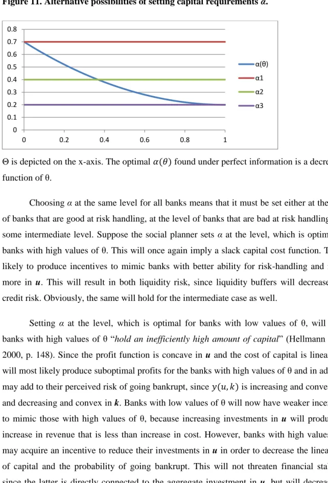
Figure 11. Alternative possibilities of setting capital requirements α. ... 32
Figure 12. The effect of stricter capital requirements on optimal adjustment of the amount of risky investment. ... 33
1
1 Introduction
Since the global financial crisis of 2008 the concept of financial stability has attracted a lot of attention of theoreticians and policy makers. Generally financial stability has been defined as
“the absence of imbalances in financial markets” (2003, Foot quoted in Haugland, Vikøren,
2006, p. 26) or as a “condition in which the financial system – comprising of financial
intermediaries, markets and market infrastructures – is capable of withstanding shocks”
(European Central Bank, 2014). The incidence of the latest financial crisis has once again demonstrated that market outcomes are inefficient posing a threat of systemic risk accumulation. Even individual bank failures “could set off a chain reaction that may
undermine the stability of the financial system” (Berger et al., 1995, p. 17). The latter may
affect sustainable economic growth and development and generates in any case a social cost in form of an economic downturn. The existence of systemic risk may therefore justify regulation of the financial sector provided that it “can improve efficiency in a way that
outweighs the costs of regulation” (Borchgrevink et al., 2013, p. 1). At the same time the
view that financial regulation is desired is not shared universally. Diamond and Rajan (2001) argue, for instance, that financial fragility is actually necessary, because it disciplines banks, while regulation may harm the economy. Nevertheless, policy makers have made several attempts at creating global regulatory framework, the most extensive being the Basel Accords. Its goal is to “ensure that financial institutions internalize the risks and explicit or implicit
costs of their business activities” (International Monetary Fund [IMF], 2012, p. 76), so that
the financial sector becomes safer and more sound. Expected to be fully implemented by 2018 the latest Basel III requirements have already been subject to discussions as to whether the financial sector is indeed heading in the direction of greater financial stability.
The purpose of this thesis is to conduct theoretical modeling of the financial sector in order to discuss possible effects of the new regulation standards and compare those to currently observed trends. This is an uneasy task, since the financial system is inherently complex and every financial institution is faced with a large number of choice variables in its decision-making process. As pointed out by Stiglitz and Greenwald (2003, p. 49), “given its equity, the bank must decide how much to lend, how thoroughly to screen loan applicants, how much to retain in government T-bills, how many funds to acquire through deposits, what
interest rate to charge on loans, and what interest rate to pay on deposits”. Only some of
2
on the belief that “capital and liquidity requirements are the main staple of financial
regulation” (Brunnermeier et al., 2009, p. 45). Hence, the thesis focuses on microprudential
regulation carrying the idea that “the robustness of the system as a whole is related to the
strength of its individual members” (Goodhart et al., 2004, p. 597).
To begin with, a comprehensive literature review on the topic of financial stability and bank regulation will be presented. Some background information on the already existing regulation of the financial sector will be given with the focus on the Basel Accords. Thereafter, a mathematical model representing an aggregation of banks will be outlined. Inspired by an article by Perotti and Suarez, the model will represent a reformulation and extension of their work. The main idea behind the theoretical construction in the present thesis is that the source of heterogeneity across financial institutions is the ability to handle risk that cannot be improved upon. Given the latter, each bank decides on the amount of risk in its asset portfolio, while the aggregate amount of investment in the risky asset defines the level of systemic risk. This model will be applied to illustrate several of the newest regulation mechanisms concerning both assets and liabilities as presented by the Basel III Accord, namely the liquidity coverage ratio, risk-weighted capital requirements and the leverage ratio. It will be shown that liquidity regulation in a combination with risk-weighted capital requirements can secure Pareto efficiency under perfect information. Under asymmetric information, however, banks will acquire incentives not to reveal their risk handling ability truthfully in order to generate higher profits. Specifically, it will be demonstrated that optimal liquidity regulation in a combination with the leverage ratio always gives banks mimicking incentives. The subsequent adjustment of risky investment as a result of such mimicking leads to a system collapse due to aggregate risk accumulation. In the case of risk-weighted capital requirements two possible alternatives will be treated: one where risk-weighted capital requirements decrease in risk handling ability and the other where risk-weighted capital requirements are set at the same level for all banks. The first case will turn out to produce same mimicking incentives and lead to excessive aggregate risk accumulation, while the second case may secure financial stability provided that capital requirements are set at a high enough level. The latter alternative will nevertheless generate a tradeoff, since banks that are good at risk handling will acquire an incentive to reduce their risky investments due to strictness of capital requirements. Finally, the thesis will compare predictions of the theoretical model with currently observed trends from the latest reports on financial stability
3 and discuss topics of optimal liquidity and capital buffers and efficiency of risk distribution as well as migration of financial activity to the non-bank sector.
4
2 Literature review
Within the topic of financial stability it has been common to distinguish between individual bank crises and system collapse as a result of aggregate risk accumulation. The latter is often formally presented as a negative externality arising, for instance, due to high riskiness of banks’ assets, excessive reliance on short-term funding or banks’ lending decisions. The existing regulation requirements aim both at making individual institutions more sound and the financial network as a whole safer. The following literature review presents models and contributions on bank crises and systemic risk modeling and proposed regulation mechanisms that could secure financial stability.
One strand of theoretical literature focuses on the problem of liquidity as a primary source of financial instability. A paper by Perotti and Suarez that inspired the present thesis constructs a model, in which “short-term funding enables credit growth but generates
negative systemic risk externalities” (Perotti, Suarez, 2011, p. 3). The authors suggest that by
borrowing short banks are subject to refinancing risk, because “sudden withdrawals may lead
to disruptive liquidity runs” (ibid., p. 4). The paper proposes liquidity regulation as a solution
to such risk and compares the effectiveness of price and quantity mechanisms. It turns out that when “banks differ only in capacity to lend profitably” (ibid., p. 5), the regulator may effectively use Pigovian taxation in order to correct for the existing externality. On the other hand, when banks differ in risk-taking incentives, “such gambling incentives are not properly
deterred by levies, while quantity constraints are more effective” (ibid., p. 6). An influential
paper by Diamond and Dybvig (1983) points out that financial institutions suffer from a maturity mismatch investing long and borrowing short. A crisis in form of a bank run may happen when “sudden withdrawals can force the bank to liquidate many of its assets at a loss
and to fail” (Diamond, Dybvig, 1983, p. 401). When such withdrawals first start, banks will
use their liquidity buffers and if those turn out to be insufficient, they will be forced to liquidate long-term assets. Since the latter can only presumably be done at some cost, the bank may go bankrupt if too many long-term assets are sold. Under this set-up bank runs are a type of Nash equilibrium, so that “even “healthy” banks can fail” (ibid., p. 402). The idea of crisis as an equilibrium is also found in other papers, such as that by Morris and Shin (2008, p. 239), who regard systemic collapse as a coordination failure and argue that “policies that lower coordination threshold or the cost of miscoordination are likely to promote system
5
experienced by several banks at the same time” (Allen, Gale, 2007, p. 149), so the idea of
systemic risk is not explicitly elaborated on. Allen and Gale (2007, p. 83) outline an alternative formulation of the Diamond Dybvig model, in which bank runs are “a natural
outgrowth of weak fundamentals arising in the course of a business cycle”. In an economic
downturn, if depositors start worrying that returns on assets may be significantly lower than expected, they will withdraw their money creating panic. In this view crises are “an integral
part of the business cycle” (ibid.). A paper by Rochet and Vives (2004, p. 5) “builds a bridge
between the “panic” and “fundamentals” view of crises by linking the probability of
occurrence of a crisis to the fundamentals”. The authors argue for the existence of unique
equilibria when investors have precise information about the condition of banks’ assets. However, when such information is uncertain and subject to speculation, “there is the
potential for a coordination failure” (Rochet, Vives, 2004, p. 5). In terms of regulation the
paper suggests that “liquidity and solvency regulation can solve the coordination problem but
typically the cost is too high in terms of foregone returns” (ibid.). Of this reason regulation
must be complemented with some sort of emergent help mechanisms.
An alternative approach to financial stability is presented in a number of papers that relate it to banks’ investment decisions, particularly the riskiness of assets. A paper by Coulter, Mayer and Vickers (2013) sets up a model, in which banks choose between safe and risky investment alternatives. The latter decision generates systemic risk externality, but the level of aggregate risk may be lowered by increasing the amount of equity on the liability side. The paper shows that under some conditions, such as perfectly correlated risks of failure and no bail-outs, both taxation and capital requirements correct the externality equally well. However, “taxation increases debt funding needed per loan, which could exacerbate rather
than diminish potential externality problems” (Coulter et al., 2013, p. 2). Moreover, the
authors argue that systemic risk in the financial sector has certain special features, which make it different from other types of negative externalities. Of this reason taxation and regulation are not equivalent and “the conventional preference for capital regulation over
taxation has a sound underlying rationale” (ibid.). A preference for capital regulation is also
shared by Rafael Repullo (2002), who presents a dynamic model where banks can invest in two alternatives: safe and risky. Under this set-up two different equilibria are possible, defined as “prudent” and “gambling”, and their incidence depends on the level of competition among banks. In very competitive and very monopolistic markets only the gambling equilibrium exists, but in intermediate markets both types of equilibria are possible. Repullo
6
(2002, p. 21) considers capital requirements and deposit ceilings as regulation alternatives and suggests that “the former are always effective, while the latter may not always work”. Koehn and Santomero (1980) examine the effect of capital requirements on the riskiness of the asset portfolio chosen by an individual bank. They set up a maximization problem, in which banks find an optimal fraction of equity to risky investment. The social planner then introduces flat capital requirements in order to “lower probability of failure” (Koehn, Santomero, 1980, p. 1243). The authors show that depending on how risk averse an individual bank is, some banks may increase the amount of risky investments. This produces perverse effects in the model, since under certain conditions “the relatively safe banks become safer, while risky institutions
increase their risk position” (ibid.). Santomero and Watson (1977) point out that capital
regulation may involve a tradeoff between “the marginal social benefit of reducing the risk of the negative externalities from bank failures and the marginal social cost of diminishing
intermediation” (Herring et al., 1995, p. 22). Blum (1999) treats the effect of capital on
assets in a dynamic setting where banks are allowed to make investments in the first two periods. Depending on whether capital regulation is introduced in the second or the third time period, this has an effect on the asset composition. Specifically, introduction of capital requirements in the third (and the last) period leads to “an increase in risk” (Blum, 1999, p. 755). Gorton and Winton (1995) propose a multi-period model of banking that is solved through backward induction. The aggregate risk in the model presents itself as a sudden event and its overall level becomes known, “even though which individual banks have losses is not
known” (Gorton, Winton, 1995, p. 8) until some further date. Banks may restructure their
portfolios in response to this information. The paper seeks to outline optimal capital requirements “with the aim of reducing the chance of an individual bank failure and thus
enhancing the overall stability of the overall banking system” (ibid., p. 1). The authors come
to a conclusion that not all banks may adhere to the rules, but under certain conditions the “regulator may find it optimal to pursue policies that resemble “forbearance” – i.e. the
regulator does not close banks that have a low or negative net worth” (ibid., p. 3). Moreover,
the paper shows that raising additional capital inflicts costs on other parts of the economy, and “these costs may lead the regulator to set a capital standard lower than that called by
stability considerations alone” (Santos, 2000, p. 14). A paper by Kashyap et al. (2010)
examines the cost effect of raising capital requirements through analyzing existing empirical evidence. The authors conclude that in the short-run increased capital requirements will “lead
7 will choose to adjust through decreasing their assets rather than increasing equity. In the long-run, however, the paper argues on the basis of the Modigliani-Miller theorem that even significant increases in capital requirement will lead only to small changes in “the borrowing
costs faced by banks’ customers” (ibid.). Hence, it is competition in the financial sector and
not equity cost that makes banks take up more risk.
Another strand of literature on financial stability suggests that the main source of systemic risk may be financial interconnectedness. Acemoglu et al. (2003, p. 24) examine
“the relationship between the structure of the financial network and systemic risk”. The
authors distinguish between complete and incomplete structures and argue that financial stability may be secured by different structures depending on the number of idiosyncratic shocks. Specifically, if the number of “negative shocks is below a critical threshold, a more equal distribution of interbank obligations leads to less fragility” (ibid., p. 24). For a large number of negative shocks the opposite is true, according to the paper. The authors argue that there exists “financial network externality” (ibid., p. 25), when banks “do not take into account the fact that their lending decisions may also put many other banks … at a greater
risk of default” (ibid.). A similar model proposed by Allen and Gale focuses on “contagion
through interlinkages” (2007, p. 261) and distinguishes between complete and incomplete
structures in a similar manner. The authors conclude that the incomplete structure of financial network “promotes possibility of contagion” (ibid., p. 282), while the complete structure “has equilibria with and without contagion and provides a weaker case for the likelihood of
8
3 The Basel Accords
Regulation of the financial system has a long history. In fact, “production of (private) money has always been taxed, the seigniorage or monopoly premium on coins being the property of
the government” (Rochet, Freixas, 2008, p. 305). In the recent years various rules for financial
institutions have become so numerous and extensive that banking has been called “one of the
most regulated industries in the world” (Santos, 2000, p. 1). One of the reasons for that is a
sudden increase in the incidence of financial crises often linked to preceding liberalization of the financial sector. Until the early 1970s banks were seen as “akin to public utilities, not
commercial entities – boring, uninnovative, but safe” (Goodhart et al., 2004, p. 594). The
onset of liberalization gave rise to several booms in the industry, but ended each time in a subsequent bust. The first global attempt to increase soundness of the financial system started with the establishment of the Basel Committee on Banking Supervision (BCBS) and the conclusion of 1988 Basel Accord on capital standards later extended to Basel II and Basel III regulation requirements. The Accords were concluded and function on a purely voluntary basis representing soft law. However, “if a country refused to abide by the Accords of the BCBS, the banks of that country could have their branches, and/or subsidiaries, banned from
operating in the main financial centers” (ibid., p. 596).
The primary goal of the first Basel agreement was harmonization of capital standards in response to “concern about international banks’ financial health … and complaints of
unfair competition” (Santos, 2000, p. 17). Targeting the liabilities was considered important
for “maintaining solvency of the regulated institution” (Morris, Shin, 2008, p. 230). Capital
was categorized into two elements: Tier 1 and Tier 2. The former consisted of equity and disclosed reserves, while the latter could, for instance, include hybrid debt capital. Later amendment to the first Basel Accord defined Tier 3 capital that allowed use of subordinated debt. With the capital definition in place the framework required that “the target standard
ratio of capital to risk weighted assets should be set at 8%” (Basel Committee on Banking
Supervision [BCBS], 1988, p. 14) for banks with an international presence. Four different risk weights, also called buckets, were designed and attached to on-balance sheet assets, while “off-balance sheet contingent contracts, such as letter of credit, loan commitments and derivative instruments … needed to be first converted to a credit equivalent and then
multiplied by the appropriate risk weight” (Santos, 2000, p. 17).This became known as the
9 safer banks the incentive to distinguish themselves from riskier ones in order to save on
capital” (ibid., p. 19).The Accord was amended in 1996 allowing banks to use their internal
models to determine required capital needed to cover risks and estimate the individual probability of default. Even though it was observed that “the introduction of Basel I was
followed by an increase in capital ratios” (Jablecki, 2009, p. 20), this proved to be
insufficient in order to guarantee financial stability.
The search for mechanisms that would improve banks’ risk management and secure truthful revelation of risks led to a proposal to revise the original Basel Accord. This prompted an introduction of the Basel II framework based on three pillars: minimum capital standards, a supervisory review process and effective use of market discipline (BCBS, 2006). The first pillar aimed at “making capital charges more correlated with the credit risk of the
bank’s asset” (Santos, 2000, p. 21). To this end a new Internal Ratings-Based Approach
(IRBA) was introduced allowing banks to estimate their own probability of default that could be converted to minimum capital requirements. The underlying idea was that “banks have
better information regarding their own risks and returns than the regulator does” (Rochet,
Freixas, 2008, p. 323). Thus, Basel II permitted banks “a choice between two broad
methodologies for calculating their capital requirements for credit risk” (BCBS, 2006, p. 19):
a somewhat modified Standardized approach or the IRBA. The second pillar consisted of monitoring process in order to “ensure that a bank’s capital position is consistent with its
overall risk profile and enable early intervention” (Santos, 2000, p. 21). Its goal was to
prevent capital from falling below some minimum level. Finally, the third pillar sought to
“encourage market discipline by developing a set of disclosure requirements” (BCBS, 2006,
p. 226) allowing “market participants to assess key pieces of information on the scope of application, capital, risk exposures, risk assessment processes, and hence the capital
adequacy of the institution” (ibid.). With such information publicly available market
participants were encouraged to influence banks’ risk management in a manner of a natural regulation mechanism. However, also these requirements proved to be insufficient: “many institutions had equity amounting to 1-3% of their balance sheets even as they were vaunting
themselves as having 10% “core capital” (Hellwig, 2010, p. 3), and various sorts of
adjustments became widespread.
Recognition of the shortcomings of the Basel II framework in the aftermath of the latest financial crisis led to a new revision process and the introduction of the Basel III
10
regulatory standard aimed at extension of previous requirements. Insuffiency of existing capital buffers was ascribed to “various deficiencies of risk models and risk management” (Hellwig, 2010, p. 5). Several new mechanisms were proposed as a strategy of improving matters. To begin with, the new framework launches harmonization of the definition of capital specifying explicitly types of capital allowed in the two Tiers and abolishing the concept of Tier 3. The new capital requirements raise the amount of common equity in the previous risk-weighted requirements and introduce additional buffers, such as “capital conservation buffer”, ensuring “build-up of adequate buffers above the minimum that can be
drawn down in periods of stress” (BCBS, 2011, p. 6). As an additional measure against
insufficiency of bank capital the Basel III framework introduces the concept of the “leverage ratio”, defined as the proportion of Tier 1 capital to total consolidated assets, and set at the 3% level. Moreover, the new regulatory standard addresses the issue of procyclicality underlining that “one of the most destabilizing elements of the crisis has been the procyclical amplification of financial shocks throughout the banking system, financial markets and
broader economy” (ibid., p. 5). This is dealt with through introduction of counter-cyclical
capital buffers that can “achieve the broader macroprudential goal of protecting the banking
sector in periods of excess aggregate credit growth” (ibid., p. 7).Finally, one of the biggest
innovations in the new regulatory framework has been regulation of liquidity through the “liquidity coverage ratio” and the “net stable funding ratio”. The former ensures that every financial institution has “sufficient high-quality liquid assets to survive a significant stress
scenario lasting for one month” (BCBS, 2013, p. 1), while the latter seeks to “provide a
sustainable maturity structure of assets and liabilities” (ibid.). Liquidity dry-up has been
pointed out as a decisive factor in the unraveling of the latest financial crisis. The two regulation mechanisms aim at preventing situations of bank runs where illiquid banks may become insolvent due to liquidity shortages. Thus, the new liquidity requirements may reflect the idea that “the traditional approach to financial regulation, based on institutional solvency and identifying solvency with equity capital, has come up short in its assigned task of
11
4 Model
4.1 Assumptions
Suppose that a bank can invest a fraction of its assets in either a safe liquid asset that, for instance, could correspond to government bonds or a risky illiquid asset u that could correspond to mortgages issued to private persons and enterprises. For simplicity it is assumed that only the risky asset generates a positive return, while the return on the safe investment is 0. Banks differ in their ability to handle risk, which is represented by the parameter θ. The latter follows some distribution with the probability density function f (θ)on the interval [0, 1]. Banks with θ = 0 are assumed to be bad at handling risk, while the opposite is the case for banks with θ = 1. Intuitively, θ could represent the quality of portfolio management, such as degree of diversification, how much time or effort is invested in monitoring loans or general ability to assess risks, i.e. human factor. Since any bank is a financial intermediary, the money for investments must come from the bank’s liabilities: in this model the choice is between equity (capital), k, and demand deposits, (1-k). It may seem that such liability structure represents an oversimplification and the existence of other types of capital has been central in discussions of financial stability. However, for emerging market economies “common equity has always been the major component of capital” (IMF, 2012, p. 92), so it may not obscure reality so much after all. It is assumed that there are unlimited borrowing possibilities in the population, so a bank can borrow any amount of money and invest in productive alternatives.
On its liabilities each bank is obliged to pay some gross promised return. For simplicity only the gross promised return on equity is regarded as positive making equity a more expensive borrowing alternative. For illustration the bank’s profit function could be written as , where u stands for the fraction of risky assets in the total assets. All banks are assumed to be of equal size with assets and liabilities summing up to 1, so u and k can thus be regarded both as fractions and as absolute amounts of risky investments and capital. The profit function is assumed to be increasing in the amount of risky investment, but decreasing in the amount of capital: and . The latter assumption implies that the Modigliani-Miller theorem doesn’t hold. The profit function is concave in
12
continuously a bank would eventually have to go “down the list”: issue loans to less and less responsible customers, which in turn affects the revenues. The effect of capital on profit is assumed to be linear, , which will be justified below. Increasing capital is assumed to have no effect on the marginal profit from the risky investment: .
It is assumed that there might exist some market discipline or “market capital requirements”. As noted by, for instance, Berger, Herring and Szegö (1995) some factors, such as costs of financial distress, make creditors demand higher interest rates. “In response, shareholders may choose to reduce these expected costs by increasing capital ratio of the
bank” (Berger et al., 1995, p. 6). A similar idea has been expressed by Piti Disyatat (2010, p.
716) who states that “a bank can issue credit up to a certain multiple of its own capital, which
is dictated either by regulation or by market discipline”. The assumption about the existence
of market capital requirements stands thus in contrast to a popular idea that “depositors are
not in a position to control the bank’s activities (or to bargain with the owners)” (Rochet,
Freixas, 2008, p. 309). In line with this assumption the fraction of capital is assumed to be a weakly increasing and concave function of risky investments: and . The promised return on the capital and demand deposits is thus held fixed in the present model allowing the amount of capital to adjust. With “market capital requirements” the profit function may be formalized as .
Aggregate investment in risky assets is assumed to generate systemic risk with a potential cost for the economy in case of collapse, c(X), where X stands for the total sum of risky investments across all banks. It is assumed that the financial system can tolerate some certain level of X treated as a stochastic variable with a certain threshold, beyond which there is significant probability of an economic turmoil. Each bank takes the aggregate risk as given and is only able to estimate its individual probability of going bankrupt . The latter increases in the amount of risky alternative, , but decreases in the amount of capital, which acts as a “buffer against unexpected losses” (Hellwig 2010: 9), . Finally, it is assumed that the function of the individual probability of going bankrupt is convex in u and k: and . The cross-derivative of this function is
assumed to be negative: increasing capital with one more unit decreases the marginal probability of going bankrupt through one additional unit of investment in the risky asset: . Each bank takes into consideration the possibility of facing systemic collapse
13 modeled as . With “market capital requirements” the function for the individual probability of going bankrupt becomes .
Both the profit function and the individual probability of going bankrupt are assumed to be functions of θ. Banks with better risk handling ability generate higher revenues from a given amount of risky investment: . At the same time the marginal probability of going bankrupt decreases in θ, , and the effect of an additional unit of capital has a stronger effect on the probability of going bankrupt for banks with high values of θ: .
4.2 A simple illustration
The following model treats the financial system as an aggregation of banks making investment and funding decisions separately from each other and not being connected by the interbank market. The starting point of the model is the net present value (NPV) of a bank,
which could be formalized the following way:
The assumptions of the model could be illustrated graphically:
Figure 1. Revenues from risky investments for different θ’s.
The fraction of risky investment, u, is depicted on the x-axis and a bank’s revenues from u are depicted on the y-axis. Higher θ contributes to higher revenues for each level of u.
0 0.5 1 1.5 2 2.5 0 0.2 0.4 0.6 0.8 1 Low value of θ High value of θ
14
The effect of k on the profit function ( ) stems from the assumption that the Modigliani-Miller theorem doesn’t hold, which in turn implies that increasing capital fraction increases banks’ total funding costs. Some empirical support of this can be found, for instance, in a paper by Bent Vale, who suggests that “an increase in bank’s equity ratio …
will increase funding costs by an interval ranging from 11 bps to 41 bps” (Vale, 2011, p. 13).
However, this argument by itself doesn’t imply the assumed linearity of the cost function. According to Vale, raising new capital may be associated with the “lemon problem”: “firms with the strongest incentive to issue new shares in the market are those firms, which are
currently overvalued” (ibid., p. 12). This will create difficulties with raising new equity and
may, perhaps, suggest a convex cost of capital. At the same time “when regulators require all banks to raise their equity ratio within a short horizon, issuing new equity in the market may
not be a significant negative signal about the true value of the individual bank” (ibid., p. 13).
Since the present thesis focuses on financial regulation, the latter argument is adopted and the capital cost function is thus assumed to be linear: ( ) .
Figure 2. Individual probability of going bankrupt, , for different θ’s.
The fraction of risky investment, u, is depicted on the x-axis. Higher θ contributes to lower probability of going bankrupt for each level of u.
0 0.2 0.4 0.6 0.8 1 1.2 0 0.2 0.4 0.6 0.8 1 Low value of θ High value of θ
15
Figure 3. Individual probability of going bankrupt, , for different θ’s.
The fraction of capital, k, is depicted on the x-axis. Higher θ contributes to lower probability of going bankrupt for each level of k.
Assuming an interior solution and since the profit function is concave in u and the function of the individual probability of going bankrupt is convex in u, the NPV function will be concave
and for a given θ have its maximum at:
This is a standard externality problem, which, in line with Perotti and Suarez (2011, p. 4), shows that “even if an individual bank’s funding decision takes into account its own exposure
to refinancing risk, it will not internalize its systemwide effect”. Since banks treat the
aggregate cost of systemic collapse as given, they naturally opt for too much risky investment in their asset portfolios. The presence of market capital requirements both reduces the marginal cost and marginal profit and the total effect depends on the strength of the two. So the market may potentially partially correct the existing externality.
0 0.1 0.2 0.3 0.4 0.5 0.6 0.7 0.8 0.9 0 0.2 0.4 0.6 0.8 1 Low value of θ High value of θ
16
5 Regulation under perfect
information
5.1 Regulation of assets
Suppose the social planner has perfect information about the distribution of θ among individual banks and can estimate the upper limit of aggregate risk that the financial system can tolerate, X, precisely. Since risky assets in the model represent mortgages, continuous lending leading to systemic risk accumulation beyond X would mean potential “excessive rise
in asset prices relative to fundamentals” (Haugland, Vikøren, 2006, p. 25). Beyond this level
many customers may start having difficulties repaying the mortgages and many banks may face unexpectedly high losses finding themselves on the verge of going bankrupt. A wave of defaults could path way for pecuniary externalities leading to price fall, which could generate further defaults. At the same time even if only some banks go bankrupt, this could have further effects through, for instance, the interbank market not modeled in the thesis. It has been observed that “the rate of growth of bank lending to the private sector has, in the past,
been a good predictor of financial crises” (Goodhart et al., 2004, p. 600).
One obvious way to ensure stability in this situation is to introduce restrictions on u, the risk-generating illiquid asset, in order “to limit the scope of the bank’s ability to engage in
moral-hazard behavior» (Hellmann et al., 2000, p. 150).
This “isoperimetric problem” can be then formulated within the framework of control theory: ∫ [ ]
̇ [ ] The Hamiltonian can be written as:
[ ( ) ]
Under appropriate concavity and boundary assumptions and for each [ ] an interior solution has to obey:
17
The function satisfies the following equation: ̇
̇
, constant, determined endogenously.
Since measures the contribution to the value function that the social planner is maximizing if was to increase with one more unit, it is reasonable to conjecture that in this case.
Note that from the first-order condition one can define , which can be inserted into the integral constraint to become:
∫ => The condition for x is:
̇ with , The condition for u becomes:
or
The marginal benefit and marginal cost are equated. Unlike individual banks the social planner accounts for the cost of the systemic risk represented by D. Looking at the optimality condition again:
, with .
Differentiating the first order condition with respect to θ yields: ̇ ̇ ̇ ̇ ̇
̇ ̇ ̇ ̇ ̇
18 Collecting terms: ̇ Since , and : ̇
The right-hand side of the expression is always negative given the assumptions above. On the left-hand side all the terms have a negative sign, except for and
. If k is weakly increasing in u, , then both and are likely to be small. In addition to that, the cross effect, , may be assumed to be weaker than the direct effects of
and . This suggests that the amount of risky investment, u, must be an increasing function of θ.
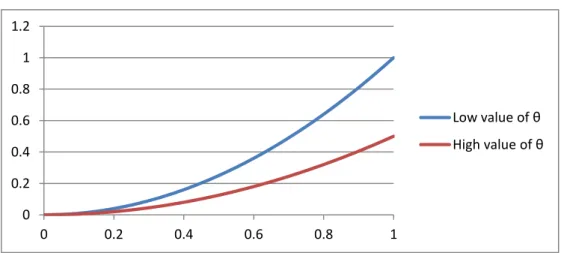
Figure 4. A possible illustration of the optimal path for
θ is depicted on the x-axis. The authorities can control this path by changing the terminal condition for x, .
The illustration above shows that the social planner will allow banks with better risk handling ability to invest more in the risky asset. However, since the social planner accounts for the aggregate risk, it is reasonable to imply that banks will be restricted in their investment decisions compared to the unregulated equilibrium. Given that “market capital requirements” decrease the optimal amount of risky investments, their strength will determine how much the assets will have to be restricted compared to the unregulated equilibrium in order to secure
0 0.1 0.2 0.3 0.4 0.5 0.6 0.7 0.8 0 0.2 0.4 0.6 0.8 1 Fraction of risky investment
19 financial stability. Since , banks with high θ and high u will also need to hold either the same or a larger fraction of capital as a result of market discipline. This suggests that will be a weakly increasing function of θ.
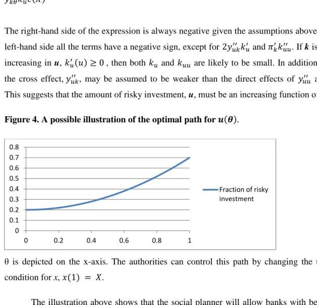
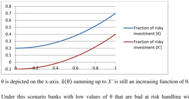
Suppose now that X is changed, set at a lower level X’. Then, since the aggregate risk is defined as ∫ , the amount of u must decrease. So if X is lowered, then the path for will also be lowered on the graph, but will still remain increasing, because different banks’ credit ability and the distribution of θ remain unchanged. Under perfect information, if X is set at a lower level, banks with low values of θ will not be allowed to operate. Graphically this implies the following shift:
Figure 5. The effect of lowering the allowed level of aggregate risk.
θis depicted on the x-axis. ̂ summing up to X’ is still an increasing function of θ.
As noted above the “liquidity coverage ratio” from Basel III “requires banks to back
their use of short-term funding with the holding of high-quality liquid assets” (Perotti, Suarez,
2011, p. 25). Since the asset side consists of just two alternatives in this model, imposing a prescription on the amount of investment in the risky asset for each bank of type θ is the same as imposing a prescription on the amount of investment in the safe alternative. So the path for
u found above could just as well be regarded as a liquidity requirement. If banks’ risk handling is perfect information, banks that are bad at risk handling would need to hold more liquidity reserves “that could be easily sold, presumably at no fire-sale loss, in case of a
crisis” (ibid.) in order to create trust and attract customers.
-0.1 0 0.1 0.2 0.3 0.4 0.5 0.6 0.7 0.8 0 0.2 0.4 0.6 0.8 1 Fraction of risky investment (X) Fraction of risky investment (X')
20
At the same time regulation of the asset side insures against liquidity but not credit risk. Illiquid assets can give unexpectedly low returns for each individual bank and losses would need to be covered with capital. Without any regulation of liabilities capital adjusts only through “market capital requirements” expressed by . If , the market has virtually no power on the banks. Without “market capital requirements” banks might still avoid investing everything in the risky alternative, because capital actually reduces the individual probability of going bankrupt. Without market power the adjustment equation becomes:
Differentiating the expression with respect to θ yields: ̇ ̇ or
̇
It is now even more obvious that u is an increasing function of θ. The optimal capital fraction
k for a given θ will be given by:
Given the assumptions about the two functions, it is clear that if a marginal reduction in the expected cost of system collapse is less than a marginal reduction in the bank’s profit from increasing capital, the bank will have an incentive to reduce its capital. Since < 0, banks that are bad at risk handling will have the biggest incentive of this kind. The individual probability of default, , could thus correspond to Internal Ratings-Based Approach used to assess credit risks. Without market discipline the amount of capital would be connected to the banks’ subjective estimates of the probability of going bankrupt. The high cost of capital might create an incentive to underestimate this probability, but even if it is estimated correctly, capital ratios will still not be connected to the amount of risky assets. So capital buffers can be optimal only by chance and might not be able to cover banks’ losses in cases of idiosyncratic shocks.
21
5.2 Regulation of liabilities
Suppose the social planner considers “market capital requirements” to be insufficient and wants to ensure stability of the system by regulating banks’ liabilities. One idea could be to tie the amount of capital to the bank’s overall assets. Since in this model kstands for the fraction of capital in the total liabilities and both assets and liabilities are equal to 1, this type of regulation could be modeled by simply making k exogenous in the optimization problem. Assuming that the social planner knows the level, at which k should be fixed, insufficiency of “market capital requirements” will result in an increase of capital buffers.
The social planner will then maximize:
∫ [ ] ̇ [ ] The Hamiltonian can be written as:
[ ] The condition for u is then:
The function satisfies the following equation: ̇
̇
, constant.
Since measures the contribution to the value function that the social planner is maximizing if was to increase with one more unit, it is reasonable to conjecture that is negative in this case.
In the first-order condition, due to assumptions about cross-derivatives of the two functions, will be unchanged, while will now be lower than in the case with “market capital requirements”. For given θ an increase in u is needed to equate both sides of the
22
expression. Regulating liabilities in this manner seems to create “incentives for banks to allocate resources to higher-risk assets because the returns on those assets were not offset by
a requirement to hold larger amounts of capital against them” (IMF, 2012, p. 116-117).
However, since aggregate risk X is determined solely by accumulation of risky assets, ̇ , an increase in u will not be allowed by the social planner, because the system will otherwise end up with the amount of aggregate risk higher than X. This suggests that the path for u should be left unchanged.
In order to deal with the incentive to invest more into risky assets the social planner may conclude that “the key determinant of the size of the required capital buffer should be the
riskiness of the bank’s assets” (Morris, Shin, 2008, p. 230). Assuming that the previously
described regulation on assets is in place, risk-weighted capital requirements could be modeled as:
or
Assuming that is a control variable as well, the new maximization problem becomes: [ ]
The solution for u is then:
, where D < 0 as previously. , which implies
for
Inserting the latter result into the first equation gives:
Differentiating the two conditions with respect to θ:
̇ ( ̇ ̇ ) ̇ ( ̇ ̇ )
23 ̇ ( ̇ ̇ ) ( ̇ ( ̇ ̇ ) ) Collecting terms: ( ) ̇ ̇ ( ) ̇ ̇
Using the fact that , and the first expression becomes ( ) ̇ ̇ or ̇ ̇ ̇
Inserting the expression for ̇ into the second expression: ( ) ̇ ̇ Collecting terms: ̇ ̇ The final result is thus:
( ) ̇
The signs of the left-hand side and the right-hand side are ambiguous. In order to arrive to formal conclusions, it will be assumed that the effect of the cross-derivative, , is weaker than the direct effects, and
24
For simplicity is set at 0:
( )
̇
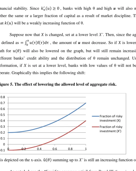
From this expression it is clear that the left-hand side of the equation is positive, while the right-hand side is ambiguous. If θ is characterized by sufficient variation in profit functions and probabilities of going bankrupt, so that the effect of – dominates, then optimal α will be a decreasing function of θ. In other words, if a marginal increase in θ increases the revenues from u and/or decreases the probability of going bankrupt from investing in u sufficiently much, then optimal capital requirements will be decreasing in θ. On
the other hand, if the effect of risky investment on the profit function and the individual probability of going bankrupt do not differ much across banks, flat or even increasing capital requirements could be optimal. In the following sufficient variation in θ with respect to profit functions and probabilities of going bankrupt is assumed. Intuitively, banks that are good at handling risk do not need the same amount of such type of buffer for the risky investments as do banks that are bad at handling risk. This is in line with the general idea in the theoretical literature on capital regulation stressing that “required equity is greatest for the riskiest
borrowers” (Coulter et al., 2013, p. 6). However, since α was originally defined as the ratio of
capital to risky investment, the fact that ̇ doesn’t imply anything about the absolute amount of capital for different banks: the latter could still be growing in θ together with the amount of risky investments.
Figure 6. The optimal path of risk-weighted capital requirements .
θ is drawn on the x-axis.
Returning back to the condition for ̇ :
0 0.1 0.2 0.3 0.4 0.5 0.6 0.7 0.8 0 0.2 0.4 0.6 0.8 1 α(θ)
25 ̇ ̇ ̇
Since ̇ , it is clear that ̇ will once again be an increasing function of θ given the assumption about the weak effect of the cross-derivative .
26
6 Regulation under asymmetric
information
The mechanisms illustrated above suggest a too rosy picture of the task faced by regulators. In a more realistic setting potential social planner would face several serious challenges. First of all, there is an estimation problem. In order to effectively regulate the asset side, the planner must know the amount of risk the system as a whole can tolerate represented by X, since this information is used to distribute risky assets among different types of banks. In reality authorities can only make estimates of the aggregate risk on the basis of growth rates of various assets and other financial indicators. In a recent report by Brunnermeier et al. (2009, p. 30) it is suggested that “financial authorities should be alerted when clear indicators of a
bubble emerge, even if the bubble cannot be identified for certain”. Secondly, such
parameters as the ability to handle risk θ, the impact of risky assets and capital on the profit function, and , and the impact of risky assets and capital on the individual probability of bankruptcy, and , are typically reported by banks themselves. If regulation is to be efficient, banks must then have an incentive to report such parameters truthfully. This represents a problem of private information.
In order to illustrate banks’ incentives, consider the regulation pattern outlined above. It was suggested that u must be following an increasing path and capital must either be tied to the risky or overall assets. If the latter is the case, then the fraction of capital is fixed, and since all banks are of equal size in the model, the absolute amount of capital kept as a buffer is the same for all types θ. In this situation banks with high values of θ, being allowed to invest more in risky assets than banks with low values of θ, will generate higher revenues. The cost of capital will be the same for all banks. This suggests that banks with high values of θ will generate higher profits. Since the probability of going bankrupt, , is increasing and convex in u and decreasing and convex in k, banks with low investments in u will face only a small marginal increase in if they increase risky investments. This creates an incentive for banks with low values of θ to pretend that they are better at risk handling than they are in reality if information about true θ is private.
The second case is a bit more challenging. If the regulator chooses to assign an increasing path for u and tie capital to risky assets, then the optimal ratio of capital to risky
27 assets is decreasing in θ, ̇ . Here a potential ambiguity arises, since banks with high values of θ have lower α, but larger investments in risky assets, so it is uncertain if they actually have more capital in absolute value compared to banks with low values of θ. Suppose that decreasing α means that banks with high values of θ hold less capital in absolute value than banks with low values of θ. Then by mimicking higher θ than what is the case in reality banks with low values of θ will face a possibility of increasing u and decreasing k. If they have relatively low investments in u and high capital buffers k to begin with, then marginal increase in u and decrease in k will produce a large positive effect on the NPV due to concavity of the profit function and a small negative effect on the individual probability of going bankrupt due to convexity of in both variables. This will create an incentive for banks with low values of θ to pretend they are better at risk handling. Suppose that decreasing α means that banks with high values of θ hold the same amount capital in absolute value as banks with low values of θ. Again, this suggests that banks with low values of θ will have incentives to pretend they are better at risk handling than they actually are. Finally, if decreasing α means that banks with high values of θhold more capital in absolute value than banks with low values of θ, then different scenarios are possible, and the conclusions will depend on the assumptions about the profit function, capital costs and effects of θ on the two functions. What is important, however, is that as long some banks receive larger profits, other banks would like to mimic them.
Suppose the social planner wants to find an optimal combination of the regulation mechanisms outlined above given informational asymmetry. Once again the NPV function of a single bank is given by:
If the social planner chooses to fix k, then, as mentioned above, banks with low values of θ and low prescribed investments in u may be willing to mimic banks with higher values of θ.
This effect will actually be reinforced if is underestimated through IRBA-modeling. Banks with high values of θ will also face an incentive to increase u due to concavity of the profit function and fixed cost of capital, but at the same time may experience a larger increase in the individual probability of going bankrupt. The situation for such banks is thus ambiguous. If banks with high values of θ do not change their investment strategy and since the aggregation of risky assets generates systemic risk in the model, the level of X is likely to
28
surpass the critical threshold. The social planner would then need to allow for less steep or even flat path of u, allowing banks with different values of θ to invest more or less the same in u. This will naturally result in ineffective risk-sharing: banks with high values of θ will have too big capital buffers as a proportion of risky assets or, alternatively, banks with low values of θ will have too small capital buffers. If k is set high enough, then banks with low values of θ may still have capital buffers that will prevent them from going bankrupt in a situation of crisis, but banks with high values of θ will end up with too much capital and suboptimal amount of risky investment. Moreover, since banks with low values of θ invest more in the risky assets than what is prescribed by the social planner, such banks will also end up with suboptimal liquidity buffers. If a large enough aggregate shock occurs, the system will need to rely on the interbank market or some sort of Lender of Last Resort, the Central Bank.
Alternatively, if the social planner chooses to combine regulation of assets with risk-weighted capital requirements under asymmetric information, different scenarios are possible. The crucial assumption here is what ̇ means for the absolute amount of capital. Recall that , and ̇ . Decreasing α is thus compatible with decreasing, unchanged and increasing k. However, as pointed out previously, both decreasing and unchanged k lead to a situation where it may become attractive for less capable banks to mimic banks that are better at risk-handling, which will consequently pose a threat to financial stability. Consider therefore the case where the social planner imposes ̇ as a capital requirement, which still means that k is growing in α. The cost of capital is linear, while the profit function is concave in u. This generates an ambiguous situation. For simplicity an illustration of what better risk handling implies for the profit function is provided.
29
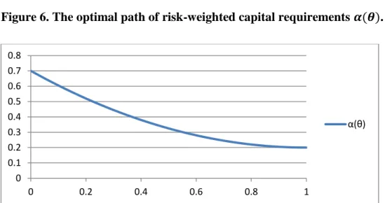
Figure 7. The effect of higher θ on optimal choice of the amount of risky investment.
The fraction of risky investments, u, is depicted on the x-axis, while revenues from u and the cost of capital k are on the y-axis.
Profit considerations may deter banks with low values of θfrom mimicking those with higher values of θ, simply because increasing risky investment given their risk handling may produce suboptimal or even negative NPV. This is because the cost of capital grows faster than the revenues from u. Since the individual probability of going bankrupt is increasing and convex in u and decreasing and convex in k, increasing both capital and the fraction of risky investments will at some point add negatively to the NPV. Banks will prefer the level of u
corresponding to the biggest wedge between the revenues from u and the cost of capital k
corresponding to maximum profit. However, if a bank with low value of θ is only allowed to make a small investment in u that it itself regards as suboptimal, then such bank will have an incentive to mimic banks with better risk handling both because marginal profit would exceed marginal cost of capital and because with very low investment in u increasing both risky investments and capital decreases the individual probability of going bankrupt. In other words, for low levels of investment in u, increasing both u and k is likely to contribute positively to the NPV through the individual probability of going bankrupt. The question is then, which level of u the bank will regard as optimal. Obviously, it must be the amount of investment corresponding to the unregulated equilibrium. As it has been pointed out before, regulation of assets entails lower investments in risky assets than under unregulated equilibrium especially for banks with low values of θ.
In order to secure an increasing path of risky investments and decreasing path of capital requirements, the social planner should opt for a high value of α for banks that are bad at risk handling and for a low value of α for banks that are good at risk handling. A high value
0 0.5 1 1.5 2 2.5 0 0.2 0.4 0.6 0.8 1
Revenues for low value of θ
Revenues for high value of θ Cost of capital