Visualization for Structured Constraint Satisfaction Problems
Xingjian Li
1and Susan L. Epstein
1,2Department of Computer Science
1
The Graduate Center and2Hunter College of The City University of New York New York, NY 10065 USA
[email protected], [email protected]
Abstract
Constraint satisfaction problems are mathematical models of real-world problems. In contrast to randomly generated arti-ficial problems, real-world problems usually have non-random structure. Knowledge about that structure, when identified in advance, can make search to find solutions more effective. This paper introduces DrawCSP, a visuali-zation program that can show both the original and the dis-covered structure of constraint satisfaction problems. DrawCSP provides insight into both search algorithm de-sign and into the challenges real-world problems present.
Introduction
Constraint satisfaction is a paradigm that applies to many challenging real-world problems, including planning and scheduling. Traditionally, algorithms and heuristics to solve constraint satisfaction problems (CSPs) have drawn both inspiration and guidance from visualizations called
constraint graphs. As solvers tackle more challenging
problems, however, these visualizations become larger and more opaque. The thesis of this paper is that, because real-world problems have non-random structure, proper visuali-zation can both support search algorithm design and pro-vide insight into the challenges inherent in real-world prob-lems. The principal results of this paper are several novel visualizations of structured CSPs, and the exploitation of that detected structure to improve search performance on challenging real-world problems.
Consider, for example, the driverlog problems from the Third International Planning Competition (Long and Fox, 2002). Each problem involves sets of drivers, trucks, loca-tions, and packages. The goal is to deliver packages to dif-ferent locations, and have the drivers and trucks finish at
Copyright © 2010, Association for the Advancement of Artificial Intelli-gence (www.aaai.org). All rights reserved.
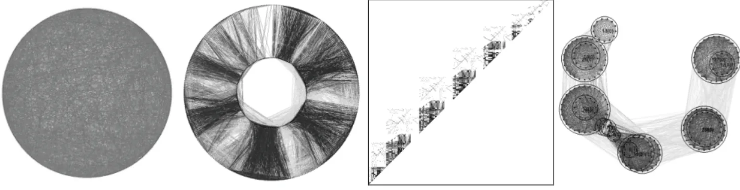
specified destinations. When cast as a CSP, a driverlog problem can be visualized as a constraint graph. The tradi-tional constraint graph in Figure 1(a), for example, plots 650 points for one driverlog problem along the circumfer-ence of a circle, and includes 17447 lines, each of which joins a pair of vertices. This picture offers little information about the structure of the problem. Figures 1(b)-1(d) are products of the program DrawCSP. They offer more strik-ing and more useful visualizations.
Formally, a CSP <X, D, C> is a set of variablesX, a set
of domains D (possible value sets for each of the
vari-ables), and a set of constraints C.Eachconstraintrestricts the simultaneous value assignment of itsscope, a subset of X. A constraint isn-aryif its scope is of sizen. This paper deals only withbinaryCSPs, those with constraints whose scopes are at most of size 2. In the constraint graph G = <V,E> for a CSP <X, D, C>,Vrepresents the variablesX, and E represents the constraints C. Thus the driverlog problem in Figure 1(a) has 650 variables and 17447 con-straints.
Thetightness tof a constraint is the percentage of value
tuples it excludes from the Cartesian product of the do-mains of its scope variables. In Figure 1 darker edges rep-resent tighter constraints. (DrawCSP actually produces diagrams in color, where tighter edges are represented with deeper colors. The figures in this paper have been adjusted for maximum contrast in grayscale printing.)
The density d of a CSP is the fraction of possible
con-straints included. Although the density of the problem in Figure 1 is less than 0.1, its many constraints mask any structure from view, at least when the variables are ar-ranged on a circle. To cope with this opacity, Figure 1(b) plots the same vertices on two concentric circles, odd-numbered vertices on the outer circle and even-odd-numbered vertices on the inner circle. (Variable numbers were as-signed by the planning competition.) Figure 1(b) reveals at
least six major, tightly-connected subproblems (darker edges) with looser (lighter) connections between subprob-lems.
Figure 1(c) is an alternative visualization of the same constraint graph as an adjacency matrix. With the lower-left corner as the origin, the x-axis andy-axis both record variable numbers. A point plotted at (x,y) represents a con-straint between variables numbered xand y, where x<y. Darker points denote tighter constraints and lighter points looser ones. In addition to the structural information that Figure 1(b) provides, Figure 1(c) makes clear that the tight subproblems form a secondary structure: a path. In Figure 1(c), subproblems are loosely connected only to neighbor-ing subproblems.
Based on such observed structural knowledge, we have designed a hybrid search algorithm. First it identifies the densely and tightly connected subproblems (clusters) shown circled in Figure 1(d), and then it solves the original problem guided by this structural knowledge (Epstein and Li, 2009b). This algorithm significantly outperforms a state-of-the-art search heuristic on real-world and bench-mark CSPs. Indeed, in some cases search becomes an order of magnitude faster.
The next section of this paper provides background on traditional CSP search algorithms and heuristics. Subse-quent sections explain how structural knowledge can guide search, describe the visualization program DrawCSP, and show the structure of various problems. Finally, we dem-onstrate improved search results with this structural knowledge.
Search for CSP Solutions
Global search for a solution to a CSP assigns a value to
one variable at a time. Global search repeatedly tries to ex-tend apartial instantiation, a set of value assignments, to a
full instantiation, where every variable is assigned a value.
Asolution to a CSP is a full instantiation that satisfies all
its constraints. During search, a future variable is one without an assigned value in the current partial instantia-tion. The (static) degree of a variable is the number of neighbors its vertex has in the constraint graph. The
dy-namic degree of a variable is the number of those
neigh-bors that represent future variables.
After each new assignment, propagation removes from the domains of the future variables any values that are in-consistent with the current partial instantiation, thus pro-ducing dynamic domains. When a dynamic domain be-comes empty (a wipeout) searchbacktracks, that is, it re-tracts previously assigned values and restores previously-reduced dynamic domains. All experiments reported here use MAC-3 propagation to maintain arc consistency (Sabin and Freuder, 1997) and chronological backtracking.
Global search iscompletebecause it either finds a solu-tion to a CSP or proves that no solusolu-tion exists. A problem is labeled “solved” if search achieves either. CSP search is usually evaluated by time (in CPU seconds) and by the number ofnodes(partial instantiations) explored.
Global search traditionally uses variable-ordering heu-ristics to select which variable to instantiate next. Many variable-ordering heuristics follow the fail first principle: address first those variables for which it is difficult to find values that lead to a solution (Haralick and Elliot, 1980). For example, a variable with a small domain and many fu-ture variables as neighbors is likely to be involved in a wipeout.MinDomDeg, the most popular traditional heuris-tic, accordingly prefers variables that minimize the ratio of their dynamic domain size to their dynamic degree. Be-cause MinDomDeg overlooks constraints’ tightness, how-ever, it can perform poorly on some CSPs with special structure, as shown below in the experimental results.
Learning can improve the quality of search heuristics when it identifies troubled variables dynamically. One way to do so is to assign a weight, initialized to 1, to every
con-(a) (b) (c) (d)
Figure 1.For the same driverlog CSP (a) an uninformative constraint graph plots variables on the circumference of a circle while (b) another constraint graph reveals more of its structure. (c) The adjacency matrix of the same graph (d) Subproblems, identified by local search, that significantly improve global search performance.
straint (Boussemart et al., 2004). Whenever, through propagation during search, a constraint causes a wipeout on a variable in its scope, that constraint’s weight is in-creased by 1. The variable-ordering heuristic MinDom-Wdeg minimizes the ratio of dynamic domain size to
weighted degree(the sum of the weights on all constraints
whose scope includes the variable). As some constraints’ weights gradually increase during search, MinDomWdeg favors variables in the scope of constraints that cause more wipeouts. At the beginning of search, however, MinDom-Wdegis identical to MinDomDeg,because all weights are 1. Therefore early search guided by MinDomWdeg is just like that guided by MinDomDeg. Because it learns,
Min-DomWdegcan eventually recover from poor initial choices
as search proceeds. Such recovery would be unnecessary, however, if these heuristics did not ignore tightness and structure.
Structure-guided search
AstructuredCSP has non-random characteristics that can
be exploited by a structure-sensitive method to outperform a more general one. For example, a composed CSP is an artificial problem that partitions its variables into con-nected components: one central componentconnected by constraints (links) to at least onesatellite. There are also constraints within satellites but no constraints between them. A class of composed problems has signature
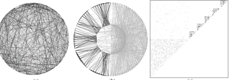
(a) (b) (c)
Figure 2.Constraint graphs for a CSP from the classComp: (a) an uninformative constraint graph (b) the actual structure of the problem showing a large, loose central component on the right and five small but tight satellites on the left (c) the adja-cency matrix constraint graph shows the central component at the lower left, the smaller satellites along the diagonal and, in the upper left, the loose links from the central component to its satellites, which are not connected to one another.
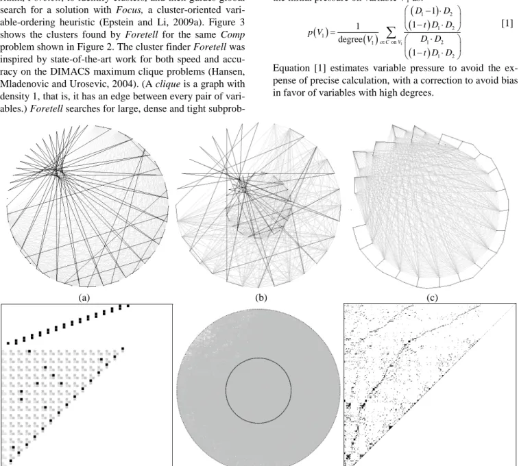
(a) (b) (c)
Figure 3. Foretellfinds clusters in the problem shown in Figure 2. Each cluster is circled; the labelx(y) denotes that it in-cludesxvariables and that it needsyadditional edges to become a clique. (a) Direct output from DrawCSP, where the five groups of clusters correspond to the five satellites (b) The nine clusters manually rearranged (c) Cluster variables are dark-ened in the adjacency matrix.
<n,k,d,t>s<n,k,d,t>dt
This specifies a central component <n,k,d,t> onnvariables with maximum domain size k, density d, and tightness t, plus s satellites <n,k,d,t> each on n variables with maximum domain sizek, densityd, and tightness t, and links between a satellite and the central component with density d and tightness t. For example, Figure 2 shows an unsolvable problem in the composed class
Comp= <100,10,0.15,0.05>5<20,10,0.25,0.50>0.012, 0.05
Structure-guided search first uses a local search
algo-rithm,Foretell, to identify clusters, and then guides global search for a solution with Focus, a cluster-oriented vari-able-ordering heuristic (Epstein and Li, 2009a). Figure 3 shows the clusters found by Foretell for the same Comp problem shown in Figure 2. The cluster finderForetellwas inspired by state-of-the-art work for both speed and accu-racy on the DIMACS maximum clique problems (Hansen, Mladenovic and Urosevic, 2004). (Acliqueis a graph with density 1, that is, it has an edge between every pair of vari-ables.)Foretellsearches for large, dense and tight
subprob-lems that either are cliques or near-cliques. (Anear-clique is a graph with density very close to 1. Note, for example, the missing edges in the clusters of Figure 3(b).) Whereas the maximum clique algorithm relies on variable degree,
Foretellrelies on the notion of pressure. Thepressureon a
variablev,given all the constraints upon it, is the probabil-ity that when one of v’s neighbors is assigned a value, at least one value will be excluded from v’s domain. For a constraint with tightnesstbetween variablesV1andV2with domain sizes D1 andD2, respectively, Foretell calculates the initial pressure on variableV1as:
1 1 2 1 2 1 on 1 2 1 1 2 1 1 1 degree 1 c C V D D t D D p V D D V t D D
[1]Equation [1] estimates variable pressure to avoid the ex-pense of precise calculation, with a correction to avoid bias in favor of variables with high degrees.
(a) (b) (c)
(d) (e) (f)
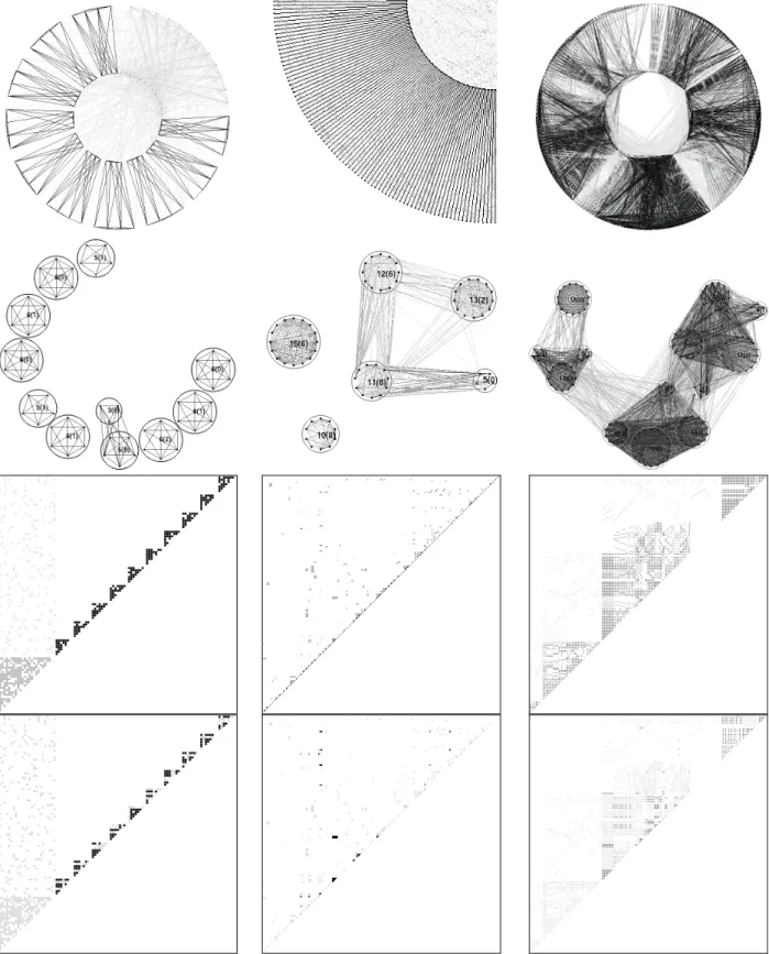
Figure 4.Examples of DrawCSP. Constraint graphs for BlackHole-4-4-e-0_ext.xml (a) with variables arranged on a single circle or (b) arranged on two circles and (c) after manual arrangement to reveal its structure, which includes a large tree and 5 short paths of length 2. (d) BlackHole-4-4-e-0_ext.xml displayed in the adjacency matrix mode. (e) Constraint graph on two concentric circles for a large optical network problem and (f) its adjacency matrix.
OnceForetelldetects the clusters,Focusrestricts search to one cluster at a time, and uses MinDomWdegto break ties within that cluster. Focus selects a cluster with the minimum ratio of dynamic domain size to original domain size for all future variables in the cluster. This ratio dy-namically estimates the extent to which tuples have been eliminated as possible cluster solutions, another application of the fail-first principle. Table 1 demonstrates that struc-ture-guided search significantly outperforms both
Min-DomDegand the adaptiveMinDomWdeg.
Related structure-based work in CSP includes identifica-tion and exploitaidentifica-tion of tractable (Dechter and Pearl, 1987; Gyssens, Jeavons and Cohen, 1994; Mackworth and Freuder, 1985) and complex structures (Gompert and Choueiry, 2005). Unlike clusters, however, that work ig-nores tightness along individual constraints, the crucial dis-tinction between the satellites and the central component in aCompproblem.
DrawCSP, a CSP visualization program
DrawCSP is a small, portable CSP visualization program, written in C++ with OpenGL and the OpenGL Utility Toolkit (GLUT). DrawCSP accepts a CSP in XCSP format (Roussel and Lecoutre, 2008), which is essentially a vari-ant of XML. DrawCSP uses the XML parser from (Berghen, 2009). There are two drawing modes; the graph mode that produced Figures 2(a) and 2(b), and the adja-cency matrix mode that produced Figure 2(c).In the graph mode, DrawCSP variables can be plotted either on one circle or on two concentric circles. The two-circle arrangement sometimes displays constraints between geometrically close variables more effectively than the single circle arrangement, as it did in Figures 1(b) and 2(b). The user can also manually move variables on the screen, and variables’ coordinates can be saved to files for future re-display. Figures 4(a-c) show a black hole CSP (Gent et al., 2007) plotted on one circle, on two concentric circles, and after manually rearrangement.
In the adjacency matrix mode, a constraint with scope variables numberedxandy, x<y,is displayed with coor-dinates (x,y). Manual rearrangement of constraints is not allowed in matrix mode. Although a constraint graph rep-resents a CSP, it can be difficult to detect the actual struc-ture when the number of constraints is large or the density of the CSP is high. Because constraints do not overlap on the adjacency matrix presentation, an adjacency matrix may better clarify relationships and thereby provide more structural information. Figure 4(d), the adjacency matrix of the same problem shown in Figures 4(a-c), shows the prob-lem’s structure without any manual re-arrangement.
Fig-ures 4(e) and (f) are, respectively, the double-circle con-straint graph and the adjacency matrix of a large optical network problem with 778 variables and 12876 constraints. No structure is visible in its constraint graph, but Figure 4(f) suggests that this problem has approximately three long paths of variables.
DrawCSP visualizes clusters when a cluster formation file (generated by the solver during search) is provided. If it is in graph mode, DrawCSP draws only the clusters, with the radius of each cluster proportional to the number of variables it contains. The center of each cluster’s circle is the geometric center of all the vertices it includes, with their coordinates computed from what would have been their single-circle locations. The geometric center is se-lected to preserve the relative positions of the subproblems, as presented by clusters, in the entire CSP graph. For ex-ample, the clusters shown in Figure 1(d) closely represent their corresponding subproblems in Figure 1(b). Supported manual rearrangement of clusters includes translation and rotation. In adjacency matrix mode, DrawCSP plots con-straints that are inside clusters darker than out-of-cluster constraints (Figure 3(c)).
Visualization and search results
The experiments reported in this section compare the state-of-the-art learning heuristicMinDomWdegagainstForetell
with Focus, and use MinDomWdeg to break ties within
clusters. To control for the vagaries of local search, ex-periments withForetellare always averaged across 10 tri-als for each problem. All experiments were run with the constraint solver ACE (Epstein, Freuder and Wallace, 2005). On each problem, Foretell was given a short time limit, usually less than 500 milliseconds, to find a cluster.
Foretell identified as many clusters as it could until it
could not find a cluster of size at least 3. The time that
Foretelluses to find clusters is included in the performance
measurements in Table 2.
Table 1: Structure-guided search speeds traditional heuris-tics on 50Compproblems by more than an order of magni-tude. Average and standard deviation are shown for search tree nodes and for time in CPU seconds, including time for cluster detection. Search is restricted to 1800 seconds.
MinDomDegfails to solve all but two instances; the other
two heuristics solve all 50 problems. Boldface denotes re-sults that are statistically significantly better at the 95% confidence level.
Heuristic Time Nodes
MinDomDeg 1728.16 (355.88) 285751.97 (61368.70)
MinDomWdeg 83.58 (38.96) 12519.36 (5811.37)
composed-25-10-20-1_ext.xml rlfap_scene11.xml driverlogw-08c-sat_ext.xml C o n st ra in t g ra p h s C lu st er s id en ti fi ed b y F o re te ll A d ja ce n cy m at ri ce s C lu st er s in ad ja ce n cy m at ri ce s
Figure 5. Constraint graphs, adjacency matrices and identified structures for a problem in composed-25-10-20-1_ext.xml, and for rlfap_scene11.xml and driverlogw-08c-sat_ext.xml. For clarity, only the lower-left quarters of the figures are shown for rlfap_scene11.xml’s cluster graph, adjacency matrix and clusters within its adjacency matrix, and for driverlogw-08c-sat_ext.xml’s adjacency matrix and clusters within its adjacency matrix.
Heuristics were compared on all the classes of composed problems on the benchmark website (Lecoutre, 2009), where there are 10 problems per class. A problem de-scribed there bya-b-cdenotes a central component witha variables, b satellites of 8 variables each andc links. All variables have domain size 10, with constraint tightness 0.150 within the central component and 0.050 on each link. Constraint density within a satellite is always 0.786. The upper section of Table 2 shows the results on these classes (together with Comp). On seven classes, structure-guided search provided an order of magnitude speedup.
The lower section of Table 2 shows the results on the three most difficult driverlog problems and on scene11, a Radio Link Frequency Assignment Problem (RLFAP) (Murphey, Pardalos and Resende, 1999). An RLFAP in-volves hundreds of radio broadcasting facilities with lim-ited broadcasting frequencies. If the frequencies of two geographically close broadcasting facilities are too close numerically, their signals will interfere with one another and communication will be distorted. Thousands of such pairs of broadcasting facilities in France are susceptible to interference. An RLFAP represents radio broadcasting fa-cilities as variables, and restricts their frequencies with constraints between pairs of variables. The domain of an RLFAP variable is the set of radio frequencies that a facil-ity can be assigned. A solution to an RLFAP CSP is equivalent to the establishment of interference-free com-munication. Scene11 is the most difficult solvable RLFAP problem.
While these pictures support improved search perform-ance, they also leave many questions for future investiga-tion. For example, the RLFAP problem has tight con-straints between every pairViandVi+1where i is an even
number. This is why the double-circle constraint graph re-sembles a sun with rays of light. The clusters thatForetell detects are also bipartite on tight edges. It would be inter-esting to study whether the structure of evenly distributed tight constraints makes this problem difficult. As another example, the constraint graph and the cluster graph of driverlogw-08c in Figure 5 show that a subproblem can be covered by more than one cluster. This observation raises questions about the possibility that some order should be imposed on how subsets of clusters are visited during search.
The semantics of tight subproblems (darker) in a con-straint graph are only sometimes available for inspection. For example, composed problems were designed and gen-erated to mislead traditional variable-ordering heuristics, such as MinDomDeg, to the loose central component, al-though the actual contention is in the tight satellites. Se-mantics for the tight subproblems in the driverlog problems are not provided.Foretell, however, does not rely on prob-lem semantics. It looks instead for structure that is likely to be contentious during search. When the problem is solv-able,clustersprovide guidance for a more effective search. When the problem is unsolvable, clusters provide an ac-cessible description of the unsolvable core and thereby suggest areas that might berelaxed, that is, made easier to satisfy, so that the problem has a solution. Relaxation could add values to the domains of core variables or accept more value pairs for core constraints.
Conclusion
This paper presents DrawCSP, a visualization program for constraint satisfaction problems. DrawCSP can display a
Table 2: Preference for variables in clusters improves search. Problem identifiers above the line are from (Lecoutre, 2009). For example, the first class is <25, 10, 0.67, 0.15> 10 <8, 10, 0.79, 0.50> 0.01, 0.05. Full descriptions are available in (Lecoutre, Boussemart and Hemery, 2004). All data forForetellwithFocusare averaged across 10 runs, and show mean and standard deviation.At the 95% confidence level, Foretell + FocusoutperformsMinDomWdegon these problems. Order of magnitude improvements overMinDomWdegare in boldface.
MinDomWdeg Foretell + Focus Time Foretell + Focus Nodes
Problems d t d Number of
instances Time Nodes
25-10-20 0.667 0.50 0.010 10 2.49 670.10 0.88 0.47 192.07 149.88 25-1-80 0.667 0.65 0.010 10 0.95 308.00 0.26 0.25 94.50 71.81 75-1-80 0.216 0.65 0.133 10 2.32 595.20 0.37 0.17 181.40 21.69 25-1-2 0.667 0.65 0.010 10 1.01 553.00 0.02 0.00 41.40 1.36 25-1-25 0.667 0.65 0.125 10 0.91 465.70 0.04 0.02 41.60 1.29 25-1-40 0.667 0.65 0.200 10 1.10 473.80 0.07 0.02 41.50 1.21 75-1-2 0.216 0.65 0.003 10 3.33 1171.70 0.04 0.01 91.60 1.50 75-1-25 0.216 0.65 0.042 10 3.29 1084.40 0.15 0.12 91.40 1.29 75-1-40 0.216 0.65 0.067 10 2.97 960.90 0.15 0.14 91.30 1.28 Comp 0.150 0.50 0.120 50 83.58 12519.40 4.31 2.41 497.96 324.33 RLFAP scene 11 — — — 1 40.74 2810.00 16.00 0.07 978.00 0.00 Driverlogw 02 — — — 1 19.49 1862.00 6.08 2.14 507.80 223.11 Driverlogw 08c — — — 1 101.58 4820.00 21.09 0.28 967.80 0.42 Driverlogw 09 — — — 1 634.03 15987.00 303.52 4.31 7847.10 153.74
CSP in two different ways. Each of them provides a direct view of the problem that may help design structure-oriented search algorithms for its solution. DrawCSP can also display the structure identified by solvers like ACE in a picture that users can easily verify and compare with the problem’s original structure.
Visualization of identified structure supports the design and improvement of search heuristics that exploit such structure. The constraint graph, the adjacency matrix, and the cluster graphs provide abstractions of the problem. They improve users' understanding of the internal structure and suggest possible alternative ways to model the problem if it proves too costly to solve. The structure observed in DrawCSP output inspired the design of a structure-guided search algorithm for constraints solvers, one which achieves significant performance improvement over a state-of-the-art search heuristic on structured problems.
Acknowledgements
We thank our collaborators at the Cork Constraint Compu-tation Centre for their continued support and involvement, particularly Eugene Freuder and Richard Wallace. This work was supported in part by the National Science Foun-dation under award IIS-0811437.
References
Berghen, F. V. 2009. "Small, simple, cross-platform, free and fast C++ XML Parser." from http://www.applied-mathematics.net/tools/xmlParser.html.
Boussemart, F., F. Hemery, C. Lecoutre and L. Sais 2004. Boosting systematic search by weighting constraints. In Proceedings of the Sixteenth European Conference on
Ar-tificial Intelligence (ECAI-2004), 146-150. Valencia,
Spain.
Dechter, R. and J. Pearl 1987. The cycle-cutset method for improving search performance in AI applications. In
Pro-ceedings of Third IEEE on AI Applications, 224-230.
Or-lando, Florida.
Epstein, S. L., E. C. Freuder and R. J. Wallace 2005. Learning to Support Constraint Programmers.
Computa-tional Intelligence21(4): 337-371.
Epstein, S. L. and X. Li 2009a. Cluster Graphs as Abstrac-tions for Constraint Satisfaction Problems. The Eighth Symposium on Abstraction, Reformulation and Approxima-tion(SARA), Lake Arrowhead, California
Epstein, S. L. and X. Li 2009b. Search on Constraint Satis-faction Problems with Sparse Secondary Structure.
Inter-national Symposium on Combinatorial Search, Lake
Ar-rowhead, California
Gent, I., C. Jefferson, T. Kelsey, I. Lynce, I. Miguel, P. Nightingale, B. M. Smith and S. A. Tarim 2007. Search in the patience game 'Black Hole'.AI Communications20(3): 211-226.
Gompert, J. and B. Y. Choueiry 2005. A Decomposition Techniques For CSPs Using Maximal Independent Sets And Its Integration With Local Search. In Proceedings of
FLAIRS-2005, 167-174. Clearwater Beach, FL, AAAI
Press.
Gyssens, M., P. G. Jeavons and D. A. Cohen 1994. De-composing constraint satisfaction problems using database techniques.Artificial Intelligence66(1): 57-89.
Hansen, P., N. Mladenovic and D. Urosevic 2004. Variable neighborhood search for the maximum clique. Discrete
Applied Mathematics145: 117-125.
Haralick, R. M. and G. L. Elliot 1980. Increasing Tree-Search Efficiency for Constraint Satisfaction Problems.
Artificial Intelligence14: 263-313.
Lecoutre, C. 2009. "Benchmarks - XML representation of CSP instances" from
http://www.cril.univ-artois.fr/~lecoutre/benchmarks.html. Lecoutre, C., F. Boussemart and F. Hemery 2004. Back-jump-based techniques versus conflict-directed heuristics.
InProceedings of ICTAI, 549-558.
Long, D. and M. Fox. 2002. "The Third International Plan-ning Competition." from
http://www.cs.cmu.edu/afs/cs/project/jair/pub/volume20/lo ng03a-html/node37.html.
Mackworth, A. K. and E. C. Freuder 1985. The Complex-ity of Some Polynomial Network Consistency Algorithms for Constraint Satisfaction Problems.Artificial Intelligence 25(1): 65-74.
Murphey, R. A., P. M. Pardalos and M. G. C. Resende 1999. Frequency assignment problems.Handbook of
Com-binatorial Optimization. Du, D. Z. and P. M. Pardalos,
Kluwer Academic Publishers, Netherlands.
Roussel, O. and C. Lecoutre. 2008. "XCSP 2.1: a format to represent CSP/QCSP/WCSP instances." from
http://www.cril.univ-artois.fr/~lecoutre/benchmarks.html. Sabin, D. and E. C. Freuder 1997. Understanding and Im-proving the MAC Algorithm. InProceedings of Principles
and Practice of Constraint Programming (CP1997),