GEM-PSO: Particle Swarm Optimization Guided by Enhanced Memory

(1)

Bowdoin College Bowdoin College

Bowdoin Digital Commons

Honors Projects Student Scholarship and Creative Work

2019

GEM-PSO: Particle Swarm Optimization Guided by Enhanced

Memory

Kevin Fakai Chen

Bowdoin College, zephyrembyr@gmail.com

Follow this and additional works at: https://digitalcommons.bowdoin.edu/honorsprojects

Part of the Artificial Intelligence and Robotics Commons, Numerical Analysis and Scientific Computing Commons, and the Theory and Algorithms Commons

Recommended Citation Recommended Citation

Chen, Kevin Fakai, "GEM-PSO: Particle Swarm Optimization Guided by Enhanced Memory" (2019). Honors Projects. 103.

https://digitalcommons.bowdoin.edu/honorsprojects/103

This Open Access Thesis is brought to you for free and open access by the Student Scholarship and Creative Work at Bowdoin Digital Commons. It has been accepted for inclusion in Honors Projects by an authorized administrator

(2)

B

OWDOIN

C

OLLEGE

A

N

H

ONORS

P

ROJECT FOR THE

D

EPARTMENT OF

C

OMPUTER

S

CIENCE

GEM-PSO: Particle Swarm Optimization

Guided by Enhanced Memory

Author:

Kevin Fakai C

HEN

Advisor:

Professor Stephen M

AJERCIK

Bowdoin College, 2019 c

(3)

Acknowledgements

I would like to express my sincerest gratitude to my research advisor, Professor Stephen Majercik. This year-long project truly would not have been possible without his continued guidance in many different aspects of the research process, and his crucial advice and helpfulness throughout this process. I had an amazing time working with him on this project and am incredibly thankful for the impact he has had on my years at Bowdoin.

I would also like to thank the Computer Science department, including my academic advisor, Professor Eric Chown, who provided much valuable advice during the process of writing this thesis. My time spent with the department at Bowdoin, both in and out of the classroom, directly inspired my passion for this subject. It also led to my continued love-hate relationship with coding in long hours of the night, and to making Searles 224 a veritable home away from home -experiences I will surely remember fondly.

My family has always been with me, be it through encouraging my academic endeavors, providing comfort, or simply offering their unwavering support through thick and thin. I have them to thank for so much of what I’ve accomplished and am extremely grateful for their continued support.

Finally, thank you to all my friends for their support, encouragement, and simply being there for me. They are without a doubt an integral part of what has made my time and work at Bowdoin special.

(4)

List of Algorithms

1 Standard PSO . . . 6

List of Tables

1 Additional PSO Parameter Variation . . . 15

2 List of all modifications, enumerated . . . 15

3 Combinations Passing First Filter . . . 25

4 Combinations Passing Second Filter . . . 25

5 Enumerated list of all modifications, again . . . 25

6 Personal Modifications Frequency . . . 26

7 Neighborhood Modifications Frequency . . . 26

8 List of all modifications, enumerated . . . 44

9 Benchmark functions, enumerated . . . 44

10 Neighborhoods, enumerated . . . 44

List of Figures

1 3-dimensional rendering of Rastrigin withn=2 . . . 16

2 3-dimensional rendering of Ackley withn=2 . . . 17

3 3-dimensional rendering of Ackley (zoomed in) withn=2 . . . 18

4 3-dimensional rendering of Griewank withn=2 . . . 19

5 3-dimensional rendering of Griewank (zoomed in) withn=2 . . . 19

6 3-dimensional rendering of Penalized Function 1 withn=2 . . . 20

8 3-dimensional rendering of Sphere Model withn=2 . . . 22

(6)

10 Dimension and Population Combinations for Personal-Modified PSO, 4 Past Bests,

in Rosenbrock . . . 27

11 Dimension and Population Combinations for Neighborhood-Modified PSO, 4 Past Bests, in Rastrigin . . . 28

12 Dimension and Population Combinations for Personal-Modified PSO, 4 Past Bests 29 13 Varying Neighborhood Topologies for Personal-Modified PSO, 4 Past Bests, on Griewank . . . 30

14 Varying Neighborhood Topologies for Personal-Modified PSO, 4 Past Bests, on Rosenbrock . . . 30

15 Varying Neighborhood Topologies for Neighborhood-Modified PSO, 4 Past Bests, on Griewank . . . 31

16 Varying Neighborhood Topologies for Neighborhood-Modified PSO, 4 Past Bests, on Rosenbrock . . . 32

17 Varying Neighborhood Topologies for [1, 2, 0] , 2 Past Bests . . . 33

18 Mann-Whitney Analysis of [1, 2, 0] on Rastrigin, 3 Past Bests . . . 34

19 Mann-Whitney Analysis of [0, 2, 2] on Griewank . . . 35

20 Mann-Whitney Analysis of [0, 2, 2] on Sphere . . . 35

21 Mann-Whitney Analysis of [0, 2, 2] on Rosenbrock . . . 35

22 Mann-Whitney Analysis of [0, 1, 0] on Ackley, 4 Past Bests . . . 36

24 Mann-Whitney Analysis of [0, 2, 2] and [0, 2, 3] on Penalized Function 2, 4 Past Bests . . . 38

25 Percent-Improvement Graphs, 2 Past Bests . . . 39

26 3-dimensional rendering of Rastrigin withn=2 . . . 45

27 3-dimensional rendering of Ackley withn=2 . . . 46

28 3-dimensional rendering of Ackley (zoomed in) withn=2 . . . 46

29 3-dimensional rendering of Griewank withn=2 . . . 47

30 3-dimensional rendering of Griewank (zoomed in) withn=2 . . . 47

33 3-dimensional rendering of Sphere Model withn=2 . . . 49

34 3-dimensional rendering of Rosenbrock’s Banana Function withn=2 . . . 49

35 Dimension and Population Combinations for Personal-Modified PSO, 4 Past Bests, in Rosenbrock . . . 50

36 Dimension and Population Combinations for Neighborhood-Modified PSO, 4 Past Bests, in Rastrigin . . . 50

37 Dimension and Population Combinations for Personal-Modified PSO, 4 Past Bests 51 38 Varying Neighborhood Topologies for Personal-Modified PSO, 4 Past Bests, on Griewank . . . 52

39 Varying Neighborhood Topologies for Personal-Modified PSO, 4 Past Bests, on Rosenbrock . . . 52

(7)

40 Varying Neighborhood Topologies for Neighborhood-Modified PSO, 4 Past Bests,

on Griewank . . . 53

41 Varying Neighborhood Topologies for Neighborhood-Modified PSO, 4 Past Bests, on Rosenbrock . . . 53

42 Varying Neighborhood Topologies for [1, 2, 0] , 2 Past Bests . . . 54

43 Mann-Whitney Analysis of [1, 2, 0] on Rastrigin, 3 Past Bests . . . 54

44 Mann-Whitney Analysis of [0, 2, 2] on Griewank . . . 55

45 Mann-Whitney Analysis of [0, 2, 2] on Sphere . . . 55

46 Mann-Whitney Analysis of [0, 2, 2] on Rosenbrock . . . 55

49 Mann-Whitney Analysis of [0, 2, 2] and [0, 2, 3] on Penalized Function 2, 4 Past Bests . . . 57

(8)

Abstract

Particle Swarm Optimization (PSO) is a widely-used nature-inspired optimization technique in which a swarm of virtual particles work together with limited communication to find a global min-imum or optmin-imum. PSO has has been successfully applied to a wide variety of practical problems, such as optimization in engineering fields, hybridization with other nature-inspired algorithms, or even general optimization problems. However, PSO suffers from a phenomenon known as prema-ture convergence, in which the algorithm’s particles all converge on a local optimum instead of the global optimum, and cannot improve their solution any further.

We seek to improve upon the standard Particle Swarm PSO algorithm by fixing this premature convergence behavior. We do so by storing and exploiting increased information in the form of

past bests, which we deemenhanced memory.

We introduce three types of modifications to each new algorithm (which we call a GEM-PSO: Particle Swarm Optimization, Guided by Enhanced Memory, because our modifications all deal with enhancing the memory of each particle). These are procedures for saving a found best, for removing a best from memory when a new one is to be added, and for selecting one (or more) bests to be used from those saved in memory. By using different combinations of these modifications, we can create many different variants of GEM-PSO that have a wide variety of behaviors and qualities.

We analyze the performance of GEM-PSO, discuss the impact of PSO’s parameters on the algorithms’ performances, isolate different modifications in order to closely study their impact on the performance of any given GEM-PSO variant, and finally look at how multiple modifications perform. Finally, we draw conclusions about the efficacy and potential of GEM-PSO variants, and provide ideas for further exploration in this area of study. Many GEM-PSO variants are able to consistently outperform standard PSO on specific functions, and GEM-PSO variants can be shown to be promising, with both general and specific use cases.

(9)

1

Introduction

In this section we introduce the Particle Swarm Optimization algorithm and its applications, and provide motivation for studying and improving this algorithm.

1.1

Why Study Particle Swarm Optimization?

Particle Swarm Optimization (PSO) is a nature-inspired stochastic optimization algorithm. We will discuss the nature-inspired component in the following sections and dedicate this section to the idea of optimization and its applications. Much of the usefulness of this algorithm stems from its versatility in applications and adaptability for various problems. At an abstract level (details of the algorithm will be discussed in the following section), we may consider a simple function

f(x₁,x₂,· · ·,x_n) =y (1)

with a valueyto be minimized, which is also dependent upon several parameters

x1,x2,· · ·,xn. (2)

Each parameter x_i can take a value within a certain range; in this scenario, optimization is the problem of finding the best assignment of thesex_ivalues in order to minimizey. In this problem,

Particle Swarm Optimization can be applied to f to determine an assignment of the parameters.

Through this abstraction, it is clear that there are a myriad of problems that can be reduced, restated, or adapted to be solved with Particle Swarm Optimization. For example, general mathematical functions with multiple variables and single outputs can all be optimized with PSO. Additionally, many problems in fields such as engineering have optimization problems that can be reduced to parameter assignment. These areas are where PSO can be most effectively applied. Furthermore, there are many variants of PSO adapted to solve functions with multiple outputs, which increases its functionality and usefulness.

It is important to note that PSO isstochastic. This is the antithesis of deterministic algorithms, which given the same inputs, will yield the same output. In a stochastic algorithm, probabilistic components are utilized, and therefore the solution found can (and often will) be different among different runs. However, this is often a desirable behavior. Some problems (such as those PSO is usually applied to) cannot be directly solved efficiently, or even at all. A stochastic algorithm makes no guarantee on findingtheoptimal solution, and doesn’t guarantee a specific error bound for the solution. However, in many general use cases, the algorithmalmostguarantees a solution of a certain quality, in a reasonable amount of time.

One may question what makes Particle Swarm Optimization an ideal candidate for a given problem compared to other nature-inspired or stochastic algorithms. It has been found that PSO is veryinexpensive- it is not computationally expensive compared to many other algorithms (for example, Ant Colony Optimization or Genetic Algorithms), it is not memory-intensive (space complexity is linear, in relation to the number of particles in the swarm, and linear at worst in relation to the number of variables being optimized), and it has relatively few algorithm parameters

(10)

to adjust. Ultimately, Particle Swarm Optimization is a powerful algorithm that can be applied efficiently in terms of time, space, and solution quality.

Of course, this algorithm is not without room for improvement. In the following sections we will explore some shortcomings of Particle Swarm Optimization and introduce our improvements (in the form of utilizing past bests) to increase the power and versatility of this algorithm.

(11)

2

Particle Swarm Optimization

Particle Swarm Optimization has had an extensive developmental history since its initial de-velopment in 1995 [3]. In this section, we will explore the origins of this algorithm and develop it chronologically, highlighting important improvements, until we reach the recognizable, accepted behaviors for a standard Particle Swarm Optimization algorithm.

2.1

Particle Swarm Optimization by Eberhart and Kennedy

This nature-inspired optimization technique was first developed by Russell Eberhart and James Kennedy - their original paper [3] provides the foundation for PSO as well as its inspiration. De-riving inspiration from the idea of limited communication between individuals in a group, particles in a particle swarm search for an optimal location in the solution space both individually and based on group-derived information. The algorithm consists of a swarm of particles, where each particle is free to move around within ann-dimensional space and has a particular position and velocity. These particles form the basis for the particle swarm, in which each particle manages and updates their position and velocity, and keeps track of a personal best, which is the best solution found by that individual particle so far. Particles communicate between each other in the swarm, and we refer topopulationas the entire swarm of particles as well as denoting the specific number of particles in the swarm. Particle Swarm Optimization relies on 5 basic principles.

1. Proximity principle: the population should be able to carry out simple space and time com-putations.

2. Quality principle: the population should be able to respond to quality factors in the environ-ment.

3. Principle of Diverse Response: the population should not commit its activities along exces-sively narrow channels.

4. Principle of Stability: the population should not change its mode of behavior every time the environment changes.

5. Principle of Adaptability: the population must be able to change behavior mode when it is worth the computational price to do so.

In more formal and concrete terms, the Proximity principle defines the space in which the particles reside (i.e. storing the position and velocity of any given particle in a particle swarm optimization). The Quality principle determines the existence of a function evaluation at any given point in the search space. There are many well-defined test functions [6] to measure the quality and performance of a PSO algorithm, such as Sphere, Ackley, Rosenbrock, and Rastrigin. To evaluate the fitnessof a given position in the search space, we evaluate the function given then -dimensional coordinate of that position. The principle of Diverse Response states the necessity for stochasticity in the algorithm - we are meant to understand the “excessively narrow channels” as deterministic algorithms (for example, having a swarm always produce the same output given

(12)

the same inputs). This would be unacceptable in Particle Swarm Optimization and as we will see, there are stochastic “kicks” that prevent this from happening. Principles 4 and 5 (Stability and Adaptibility) are particularly interesting in that they represent the oft-quoted exploration versus exploitation trade-off that is exhibited in so many optimization and search algorithms. Stability pushes us towards not deviating greatly from what could be an optimal solution, while Adaptibility urges the algorithm to explore nearby spaces and change its behavior in order to find potentially better solutions.

In the original PSO algorithm, the limited communication between individual particles is fa-cilitated through the personal best (kept track of by each individual particle), and the global best, which is determined through examining the personal best of all the particles at any given time. Ad-ditionally, each particle has a velocity whose update is determined by a stochastic factor multiplied by the vector from the particle’s position towards the particle’s personal best position (influencing the velocity vector) and another stochastic factor multiplied by the vector from the particle’s posi-tion towards the swarm’s global best posiposi-tion. The update equaposi-tion can be expressed as follows,

(3)

vi =vi+2.05·U(0,1)·(pbesti−xi) +2.05·U(0,1)·(gbest−xi)

Where xi represents the position of the particle i. We see the beginnings of a current standard PSO algorithm in this velocity update equation. In this equation, U(0,1) represents a vector of dimension equal to the dimension of the problem space, with each index of the vector having a random value between 0 and 1, andvidenotes the velocity of particle indexedi. The 2.05·U(0,1) factors found on the pbest and thegbest components of this equation ultimately becomes the φ1

andφ2 components of the regular velocity update equation, dictating the power and influence of

the personal and neighborhood best components, respectively. The assignment of 2.05 forφ1and

φ2is an empirically determined value. Significant deviation from this value for the parameters has

been shown to lead to divergent behavior [7]. The pbest_i is the personal best location of particlei, and thegbest variable represents the best location found by the entire swarm.

A natural extension to this algorithm is to change the influence of the limited communication

factor in PSO. In the original, we have thegbest component acting as the communication among

particles in the swarm. However, we can change this communication; for example, limiting the

gbest of any given particle ito just the best solution found by the particles(i,i−1,i+1), for all the particles, causes the communication to occur among different groups and changes the way the information of personal bests is spread throughout the algorithm. Along with this change comes a renaming of variables, instead of using agbest we use annbest, denoting a neighborhood best. The group(i−1,i,i+1)is therefore referred to as the neighborhood of particlei.

In our work, we implement and experiment with the global, ring, and Von Neumann neigh-borhoods. Global neighborhoods are the same as the original standard PSO’s concept of global bests. All particles belong to one neighborhood and the neighborhood best is equivalent to the global best. The Ring neighborhood can be constructed by creating a circle of all the particles and enumerating them from 1 to n. The neighborhood of particle iis thus itself and the particles to the left and right of it, corresponding to(i−1,i,i+1). Extending this idea to a two-dimensional grid with wrap-around, we can construct a Von Neumann neighborhood, in which any particle’s neighborhood consists of itself and the particles above and below it, as well as those to the left and the right.

(13)

One paper [5] describes Inertia Weighted PSO and Constriction PSO - two tools used by the basic Particle Swarm Optimization algorithm to stop the velocities of a particle from becoming too large (and disrupting the searching of the swarm) or for the swarm system to break down over time. We first examine the inertial version. This adds a sort of “friction” to the velocity. In the original PSO we have thevi=vi+· · ·, but now we multiply theviby an inertia weight, which yieldsω·vi, whereωis the inertia weight. After this weight is applied, the rest of the velocity update proceeds as normal, taking in the personal best and neighborhood best influences on the velocity. In this equation, ωacts as an inertial restriction component (ω is the percentage of the velocity kept for the next iteration). Additionally, φ1 andφ2take on lower values (around 1.49618). The result of

inertial PSO is somewhat similar to the constriction PSO, but the lowering of the φ values has a non-negligible influence on the impact of different factors of the PSO update equation.

The other version of PSO, constriction PSO, is the one we use in our work. Instead of using the inertial weighting which applies to only the previous velocity, the constriction coefficient applies to the velocity update by being multiplied with the velocity afterthe rest of the original velocity update equation (with the personal and neighborhood bests) has already been applied. The con-striction coefficient is determined according to a formula using φ1 andφ2, the influence strength

coefficients. We use a variableχto denote the constriction coefficient, where

χ= 2

φ−2+pφ2−4φ

(4)

[5]. Additionally, we utilize the (previously found) specific constraint of φ= φ1+φ2 > 4 to

achieve optimal behavior. In the usual assignment of parameters here, φ=4.1,φ1 =φ2=2.05,

andχ=0.7298. We may choose also to limit the maximum and minimum attainable velocity (and

sometimes limit the position as well, if we wish to bound the search space strictly) in order to confine our search to a reasonable range and reduce the speed (and therefore increase the level of detail when searching) of each particle.

PSO has another important variant called fully informed particle swarm (FIPS). This is an algorithm in which each particle is affected by all of its neighbors. The velocity update equation for a given particleiis as follows:

v_i=χ vi+ 1 K_i Ki

∑

n=1 U(0,φ)⊗(pbestnbrn−xi) ! (5)

[5] whereKiis the number of neighbors for particleiandnbrnisi’snth neighbor. FIPS sometimes finds better solutions in fewer iterations than regular PSO but is more dependent on population topology. We ultimately decided not to experiment with this method, as its population topology dependence is tangential to the aspects of PSO we seek to improve, but it certainly has potential for future work.

(14)

2.2

PSO and Pseudocode

Algorithm 1:Standard PSO

input : f, function to be minimized withdimdimensions

numIter, the number of iterations to be performed

pop, the number of particles in the particle swarm

output:x, a vector representing the final position of the minimum value found in f f(x), the minimum value found in f

fori=1topopdo

Initialize particleiwith a random position and velocity

end

foriter=1tonumIterdo foreach particledo

Update particlei’s velocity,v_i

Update particlei’s position,xi

Calculate f(x_i), the fitness value for particlei’s position

if f(x_i)>best_ithen Set pbest_i= f(x_i) end if f(x_i)>nbest_ithen Setnbest_i= f(x_i) end end end

returnbest solution found over all particles i

This is an accepted, current, standard form of PSO, which we will refer to as standard PSO throughout this study.irepresents the particle index,pbestiindicates the personal best value found over all iterations so far, and nbest_i indicates the best value found over all iterations so far by particle i’s neighborhood. It utilizes the following positional and velocity update equations, re-spectively:

x_i(iter) =x_i(iter−1) +x_i(iter) (6) (7)

v_i(iter) =χ[vi(iter−1) +U(0,φ1)·(xi(iter−1)− pbesti(iter−1)) +U(0,φ2)

·(nbest_i(iter−1)−x_i(iter−1))]

Here,(iter)denotes the iteration at which we are looking at the value. This helps differentiate the new velocity and position in the update equation from the velocities and positions used in the previous iteration used to calculate the new iteration values. Again, v_i represents the velocity of particlei,xiis the position of particlei,iteris the iteration that the PSO run is currently at,χis the constriction coefficient discussed earlier, andφ1andφ2represent the personal influence component

and the neighborhood influence component, respectively. pbest_i is the personal best coordinates found by particlei, andnbestiis the best solution coordinates found by the neighborhood of particle

(15)

2.3

Issues and Improvements

One of the most important issues in a stochastic optimization algorithm is the problem of pre-mature convergence as it relates to the exploration-exploitation duality. If the exploration is too large, an algorithm may never converge on a near-optimal solution, but it will fail to search more thoroughly in better potential solution candidate spaces in favor of searching more randomly over larger areas. If we exploit our known solutions more strongly, we can end up with premature convergence, i.e. the swarm ends up all converging on a sub-optimal solution. Our work centers around the problem of premature convergence in Particle Swarm Optimization. Our approach -modify the way the algorithm uses bests, by accounting for past personal bests and past neighbor-hood bestsas well as the regular bests. Along with this we need to determine how to store these bests, how to remove the bests, and how to actually use them.

Section 3 explores the literature and research related to this area of improvement for PSO, Section 4 discusses the techniques we decided to combine and implement, and Section 5 explains our high-level testing methodology and goals. Sections 6-9 are dedicated to our detailed data collection, testing, results analysis, conclusions, and outlines goals for further research and analysis in this area.

(16)

3

Related Work

In this section we describe related work. Each of the articles mentioned explores a different aspect of incorporating past bests, ranging from determining the best method for using multiple bests to the selection of various bests to store in memory, to other advanced modifications to dif-ferent variants of PSO.

Yin, Glover, and Manuel [9] modify Particle Swarm Optimization by merging it with adap-tive memory programming techniques. Their algorithm uses a generated reference set (akin to our idea of using past bests), and systematically selects subsets of the reference set to generate new solutions. It also implements path re-linking, inspired by the idea of treating one given solution as aninitiating solution(which strongly influences other solutions) and the others asguiding solu-tions(which influence other solutions less strongly, i.e. guiding). The paper draws on intelligent learning provided by scatter search and path re-linking. One specific concept applied to increase exploration of PSO used in the paper wastabu search, which strongly weights a particle’s velocity and position in order to push against revisiting the same solutions/spaces. In the end, the paper uses the particle’s best, the swarm’s best, and the particle’s second best. Weightings are varied among three methods: equal weighting, fitness weighting, self-weighting. The paper also explores the

relationship between this weighting and dynamic neighborhoods, and uses theMinimum Diversity

Strategy, which adds a new solutionyin place ofxif and only if the solution quality ofyis better than that ofx(i.e. the function evaluation ofyis lower than that ofx), and if the minimum distance betweenyand other members satisfies a specific threshold, which can be dynamic or static. This final idea is one of the key “adding” processes we used that will be discussed in Section 4.

Shin and Kita [8] focus specifically on the implementation of the “second best” particle influ-encing the PSO algorithm. Their algorithm looks at two types of second best particles, one being the personal second best for each particle, and one being the neighborhood second best for each neighborhood. Ultimately, they find a behavior of reducing convergence toward the optimal (which is, as we have discussed, a favorable behavior of the algorithm).

(8)

v_i(iter+1) =ωvi(iter) +c1·U(0,1)·(pbesti(iter)−xi(iter)) +c2·U(0,1)

·(gbest1(iter)−xi(iter)) +c3·U(0,1)·(gbest2(iter)−xi(iter))

describes the new update equation with a second global best. In this equation, ω is the inertia weight,c₁,c₂,c₃are acceleration coefficients, withc₁,c₂determining relative pull of pbest,gbest₁, andgbest2, respectively. These constants are experimentally determined to bec1=c2=1.5. iter

is the current iteration number, andU(0,1)is randomly distributed and functions as the stochastic

element of the algorithm. Each instance of U is independently randomly generated. This can

be easily adapted to a second neighborhood best for each neighborhood which is a specific topic we will adapt further in our study. The equation for the second personal best is quite similar to the previous, with c₄ replacing c₃ and the inclusion of a second factor in the personal influence

(17)

component of the velocity update equation:

(9)

v_i(iter+1) =ωvi(iter) +c1·U(0,1)·(pbesti,1−xi(iter)) +c2·U(0,1)

·(gbest −x_i(iter)) +c₄·U(0,1)·(pbest_i_,₂−x_i(iter))

Here, ω is once again inertia weight, and c1,c2,c4 are the acceleration coefficients. t is iteration

time, and the random variableU(0,1) is uniformly randomly distributed. Each instance ofU is independently randomly generated.

Broderick and Howley [1] conducted a study with a focus on the best utilization technique given multiple stored past bests. The algorithm presented in their paper uses a specific type of weighting: the contribution of each neighbor is weighted by previous fitness. It is an improvement built upon a Fully Informed Particle Swarm algorithm called Ranked FIPS, which itself uses a ranking system to weight the influences of all the past bests. This algorithm, named PSO EMP, incorporates particles that selectively remember some best positions; the personal influence factor of the velocity update equation is replaced with a new EMP-specific term:

(10)

v_i(iter+1) =χ∗(vi(iter) +U(0,1)·EMPterm+U(0,1)·c2·(gbesti−xi(iter)))

This new equation can split the personal influence component φ1 into N equal parts, where N

represents the number of remembered positions (akin to the equal weighting idea in the previous paper). Alternatively, it can weight the bests according to a power law distribution where a saved best coordinate with a rank ofnis weighted twice as heavily as a best coordinate with a rank of

n+1. Of course, there is a third and arguably easiest-implementation option, namely just picking a random best from the saved bests. Two clean conclusions can be derived from their testing data and analysis. First, too many remembered past best positions hinders convergence, but using two particles yields good results. More than three guiding solutions blurs the total guidance of the information provided by the bests and ultimately degrades performance. Second, the paper found that roulette selection (fitness-based selection of a best) appeared to yield the best overall performance. These conclusions are all derived in the framework of exploration/exploitation -the solutions approach a balance between increasing diversity without overly hindering overall convergence.

Another interesting PSO variant, Simple Adaptive Cognition PSO, makes these modifications to the position and velocity updates:

¨

x_t₊₁=φpU⊗(pt−xt) +φgU⊗(gt−xt) (11) ˙

xt+1=ωx˙t+x¨t+1 (12)

xt+1=xt+x˙t+1. (13)

[4] Here, φp,φg are the cognitive and social coefficients (in our terminology, personal and neigh-borhood influence weights), andωacts as a momentum coefficient, set between 0.4 and 1.0. This momentum coefficient functions as an alternative to the constriction coefficient normally used in constriction PSO. This value is not unlike that used in standard inertial PSO. Simple Adaptive Cog-nition (SAC) recognizes and exploits the tendency of particles to “periodically jump far outside of

(18)

the current region of exploration” (which they dub “bursts of outliers”). The paper briefly

criti-cizes the idea of linearly decreasing momentum ωover a PSO run, despite other papers pointing

to its success. It argues instead that the linearly-decreasing momentum methodology’s success has “more to do with the fact that they happen to pass through good values during an optimization run [4].” This is also the first article to discuss the importance of a best-related statistic the authors call “information age.” Essentially, if a particle hasn’t updated its personal best in a long time then it inhabits a region of the function that does not warrant further explanation. The solution: decay the magnitude of vectors toward locations in proportion to how long ago they were discovered with a simple coefficient. Thus, the new acceleration update equation reads:

(14) ¨

x_t+1=φpγt−tpU ⊗(pt −xt) +φgγt−tgU⊗(gt−xt)

whereγ∈(0,1)is the adaptation weight, starting at close to 1.tprecords the time of last update of

p_t, the personal best, andt_gis the time of the last update ofg, the global (which can be modified to work on neighborhoods as well). Every time a particle updates its own pt, it setstp=t, and every time the neighborhood updates theg_t, it sets t_g=t. If we have no decreased weighting towards older solutions, we setγ=1 and the behavior of the algorithm exactly matches regular PSO. This is one of the more unique articles because it doesn’t directly apply the influence of the past-best in the velocity update equation so much as it interprets the age of the past best. This procedure only adds one parameter,γ, and requires very little additional memory. This can be easily incorporated in conjunction with other methods which use multiple past bests. It also introduces the idea of keeping at least 1 past best, but keeping more only if they are found withinxmaximum time-frame (i.e. if they get too old then drop the best).

PSO has been combined with other search techniques to improve performance. In particular, evolutionary operators have been used to select best particles, increase diversity, and improve ability to escape local minima. There also exists collision avoidance mechanisms that attempt to prevent local minima convergence. This final paper uses all particles’ pbeststo update velocity of any one particle. Let the superscriptddenote a specific index in the overall vector for velocity and position of a particle [10]. The algorithm uses the equation

(15)

vd_i =w∗vd_i +crand_id ∗(pbestd_f

i(d)−x d i)

where f_i defines which particles’ pbests the particle i should follow. This algorithm also uses tournament selection to learn from another particle’spbest with probabilityPc:

• Randomly choose two particles out of the population which excludes particle whose velocity is updated

• Compare fitness of the pbestsand select the better one.

• Use the winner’s pbest as an exemplar to learn from that dimension. If all exemplars of a

particle are its own pbest, randomly choose one dimension to learn from another particle’s

(19)

While we ultimately do not use this tournament selection to learn from other pbests, we do

implement tournament selection on the particle’s own selection of a pbest in order to increase

diversity without decreasing quality of solutions.

Ultimately, the most important techniques and results we derive from these articles is a distance-based metric for increasing diversity, ideas for how to utilize a second past best in conjunction or in lieu of a standard personal or neighborhood best, and borrowing genetic-algorithm inspired tech-niques for applications in Particle Swarm Optimization. Some shortcomings of these studies are their narrowed range of focus. Our ideas, which will be discussed in the following section, focus on synthesis, expansion of some of the basic ideas proposed in these articles, and developing a clearer structuring of how the algorithm interacts with its Past Best information.

(20)

4

GEM-PSO

In this section, we discuss our approach to incorporating past bests in the PSO algorithm. In our methodology, we break this process into three components: adding bests to memory, removing bests from memory, and selecting a best from memory to use. The following sections cover these three components, providing our motivation to select our specific methods, as well as how they function. When we combine these 3 modifications into a single PSO algorithm, we call the result-ing algorithm a GEM-PSO variant. PSO stands for Particle Swarm Optimization, and GEM stands for Guided by Enhanced Memory - since our algorithm stores and uses Past Bests, we consider it to have enhanced memory.

4.1

Adding Bests

In traditional PSO, the initial pbest of each particle is the particle’s initial position. Our initial-ization process is the same, but because we are using multiple past bests, our general best adding mechanism must be different. We introduce three different methods to determine when a particle or a neighborhood will add a new best to the memory. For our first adding mechanism, we draw inspiration directly from standard PSO, in which a best with a greater fitness (i.e. a lower function evaluation) replaces a best with a lesser fitness. Therefore, this modification simply saves a best when it has a greater fitness than any existing saved best in the memory.

One difficulty is that if a particle is trapped near a local optimum, or if a neighborhood was already mostly converged on a local optimum, then the adding-best modification could potentially populate the entire memory for the particle or the neighborhood with a plethora of “bests” all originating from roughly the same location. In doing so, selecting different bests from the memory would not increase diversity - they would all influence velocities toward the same local optimum location.

We developed two strategies to counter this behavior. The first is simply to only store bests based upon a random factor. Given the previously mentioned problematic situation, saving with a random probability would reduce the number of past-bests saved from that local optimum, which would additionally provide a better chance for older, more diverse past bests to remain in the memory (and not get pushed out by our newly found bests).

The other way to deal with this issue is a distance-based metric [9]. In this modification, we only save a best that resides more than a certain distance from the other bests. As discussed, this ensures that we have a good amount of variation in our past bests memory and directly negates the possibility of multiple bests being saved from a single local optimum location.

This yields our three adding modifications: saving the best (i.e. best fitness), saving with probability, and saving with a minimum distance. We will refer to these modifications with the abbreviations save-best, save-prob, and save-distance, respectively.

4.2

Removing Bests (and Cache Replacement Policies)

Caches can give us some insight into how we should approach the problem of saving n past

(21)

or nbest as a single step, we may consider the process as adding a second best to the memory,

removing one of the bests based on a removal mechanism, and then being left with the new pbest

ornbest. In the original PSO, the lesser fitness solution is removed and the greater fitness solution remains. We may adapt this policy for multiple past bests by removing the best with the lowest fitness. This is precisely the framework for our first removal modification: Remove Worst.

Studying cache replacement policy yields three ideas for removal modifications. Two of the most straightforward cache replacement policies are LIFO (Last In, First Out) and FIFO (First In, First Out). LIFO is incompatible in ideology with our algorithm. If we were to use LIFO, we would essentially remove the newest-found best (which, due to convergence is more likely to have better fitness), while holding onto an array of bests that becomes older, and therefore very likely comparatively worse in quality over time. FIFO, however, is compatible. We can adapt it to our

algorithm and implement a policy of removing the oldest found solution. On a high level, this

seems reasonable - though there is no guarantee (because of stochastic behavior), a best found in a previous iteration is more likely to be worse than a best found in a later iteration as convergence occurs. This forms the basis for our second removal modification, Remove Oldest.

In cache replacement, a strong objective is to optimize the contents such that they are the most frequently accessed (and therefore save the most time by being saved). The policy that corresponds to this is referred to as Least Recently Used (LRU). If we pair this idea with weighted or tournament selection style where we are selecting better bests more often, then we would ostensibly remove less useful bests. However, frequency of use may not pair well with our selection mechanisms (discussed in the next subsection). On the other end of policies, we have MRU (most recently used). This seems like an apt choice; we may not want to use the same bests too often and end up with premature convergence again. In order to avoid this, we should artificially diversify our past bests in order to continually have access to varying influences from our past bests, increasing exploration. This forms the basis for another policy, which we call Replace Last Used.

Finally, we may want to artificially increase diversity by injecting additionally stochasticity into our algorithm. This directly corresponds to removing a best at random when the memory is full, to accommodate a new best. This policy has no bias toward either bests with higher or lower fitness - it adds stochastic behavior evenly. We call this final removal modification Replace Randomly.

We decided upon four modifications after studying cache replacement policy, namely Replace Worst, Replace Oldest, Replace Last Used, and Replace Randomly. We refer to these modifications in the rest of the study as replace-worst, replace-oldest, replace-last-used, and replace-randomly, respectively.

4.3

Using Bests

In this paper we strongly emphasize the breaking down of the velocity update equation into two components, which are the “personal influence,” and the “neighborhood influence” components. Each of the four selection ideas we are testing can be applied to either the personal influence component, the neighborhood influence component, or both components of the velocity update equation.

(22)

In standard PSO, we simply select the only current pbest or nbest and use it, for both the personal and neighborhood influences, respectively. This still serves as a valid method for us to use in our new PSO. It is important to keep in mind that because of the adding and removing modifications we discussed previously, selecting the past best with the greatest fitness from the past bests saved in the memory does not necessarily yield the location of the past best found. For example, that best could have been removed because it was recently used, or removed randomly, or it could have not been added because of our save-distance modification. We call this Select Best.

For our other selecting modifications, we also have random selection, in which a random best is selected from those available in the memory. Again, this is a potentially desirable modification because it introduces more stochasticity (and therefore, more exploration) to the algorithm. We call this modification Select Randomly.

We also use a concept introduced in a previously mentioned article [1] by including equal weighting-based selection. In this modification, two bests are selected, and the influence compo-nent (φ1for personal,φ2for neighborhood) is split evenly between the two particles. That is, if we

applied this modification when using personal past bests, instead of aU(0,φ1)·pbest, we would

haveU(0,φ1/2)·pbest1+U(0,φ1/2)·pbest2. Notice that the twoU(0,φ1/2)terms are

indepen-dently generated and not identical. We named this modification Select with Equal Weighting. Finally, we added a tournament selection paradigm, inspired by genetic algorithms. Simply put, this modification selects two bests at random without replacement from the past bests stored in the memory. It then compares the two past bests and returns the one with better fitness (lower function evaluation). This modification balances weighting towards bests with higher fitness (as in Select Best) and random selection (as in Select Randomly). This modification is referred to as Select with Tournament Selection.

Thus, our final four selection modifications are Select Best, Select Randomly, Select with Equal Weighting, and Select with Tournament Selection. We refer to these modifications with the abbre-viations select-best, select-random, select-equal-weighting, and select-tournament, respectively.

(23)

5

Experimental Methodology

Given all of our changes to the standard PSO algorithm that we would like to test, the simplest testing paradigm is to try each combination of the saving, removing, and utilization methods, as well as varying the memory size (i.e. the number of past bests saved per particle) in our preliminary testing. We settled on these different modifications for our three different modification components (enumerated for easy reference further on).

Adding/Saving Replacing/Removing Selecting/Using

0 - Save Best (Standard) 0 - Replace Oldest 0 - Select Best (standard)

1 - Save with Probability 1 - Replaced Last-Used 1 - Select Random

2 - Save with Distance Metric 2 - Replace Worst (standard) 2 - Select 2 Past Bests

with Equal Weighting

3 - Replace Random 3 - Select with

Tournament Selection

Additionally, we need to take into account that some of these combinations may not perform optimally under standard PSO parameters, but may outperform standard PSO under other param-eter assignments. Therefore, we need to vary some of PSO’s base paramparam-eters as well.

We aim to quantitatively judge our GEM-PSO combinations by the time taken for the code to find its ultimate solution, the number of iterations it runs through before it stops improving, and the quality of the best found solution.

Table 1: Additional PSO Parameter Variation

Parameter Possible Values

# of Past Bests 2, 3, 4

Dimensions 30, 50

Swarm Size 30, 50

Function Rastrigin, Ackley, Griewank, Penalized Function 1,

Penalized Function 2, Sphere, Rosenbrock

Neighborhood Topology Global, Ring, Von Neumann

Table 2: List of all modifications, enumerated

In this paper, we will often refer to a specific set of modifications by an ordered triplets of numbers within brackets, particularly when labeling graphs or discussing many different versions of PSO with modifications. For example, standard PSO can be written as [0,2,0], and [1,2,3] would correspond to a GEM-PSO with the modifications save-prob, replace-worst, and select-tournament. This GEM-PSO that saves past bests with a certain probability, selects from the saved past bests the one with the highest fitness (minimum), and applies tournament-selection to determine which best to use.

(24)

5.1

Functions

In this subsection, we take a look at the seven different generalized n-dimensional functions that we will apply to our modifications. These functions are commonly used as benchmarks [2] to test the performance of optimization functions and algorithms.

Because all functions can be generalized to ndimensions, we are able to construct both a 30-dimensional and 50-30-dimensional variant for our data collection procedure.

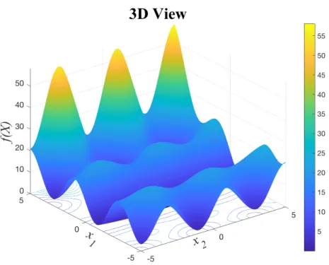
5.1.1 Generalized Rastrigin’s Function

f(X) = n

∑

i=1 x2_i −10 cos(2πxi) +10 (16) Minimum location: x_i=0∀i.

Minimum value: f(min) =0.

Rastrigin is a common and challenging benchmark function for optimization testing. The over-all behavior of the function is parabolic (bowl-shaped), with a minimum occurring around the center of the function. However, due to the cosine term, there are many local minima around the global minimum that have a tendency to cause premature, local convergence.

(25)

5.1.2 Ackley’s Path Function f(X) =−20 exp( −0.2× s 1 n n

∑

i=1 x2_i ! )−exp( " 1 n n

∑

i=1 cos(2πxi) # ) +20+e(1) (17) Minimum location: x_i=0∀i. Minimum value: f(min) =0.

Ackley’s Path Function (also known as Ackley’s Function No. 1) is another standard test func-tion for benchmarking optimizafunc-tion algorithms. This funcfunc-tion initially appears similar to Rastrigin, but differs in that while the previous function’s slope becomes more gradual when approaching the optimum, Ackley becomes progressively steeper, resembling a more conical shape. Again, the local behavior is oscillatory which creates many local optimum, presenting an opportunity for premature convergence.

(26)

Figure 3: 3-dimensional rendering of Ackley (zoomed in) withn=2

5.1.3 Generalized Griewank’s Function

f(X) = 1 4000 n

∑

i=1 x2_i − n

∏

i=1 cos xi √ i +1 (18) Minimum location: x_i=0∀i. Minimum value: f(min) =0.

The Generalized Griewank’s Function is a slightly less commonly used, but still well-known benchmark function. It resembles Rastrigin except the local optima are much more densely packed in the function in comparison - meaning more local optima but a smaller radius of strong “pull” for any given particle around that minimum coordinate.

(27)

Figure 4: 3-dimensional rendering of Griewank withn=2

(28)

5.1.4 Generalized Penalized Function No. 01 f(X) =π n× ( 10 sin2(πy1) + n−1

∑

i=1 (y_i−1)21+10 sin2(πyi+1) + (y_n−1)2 ) + n

∑

i=1 u(x_i,a,k,m) (19) Minimum location: x_i=−1∀i.

Minimum value: f(min) =0.

The Generalized Penalized Function No. 01 has a markedly different appearance from the previous few functions. It is the juxtaposition of increasing-magnitude peaks and troughs when

viewed in the positivexdirection, with increasing-magnitude peaks and troughs when viewed in

the positiveydirection as well. This presents entire lines of points of local convergence that present difficulties for optimization algorithms to “escape” (and explore outside). Note that the optimum location is wherexi=−1, rather than at 0 like the previous functions.

(29)

5.1.5 Generalized Penalized Function No. 02 (20) f(X) =0.1× ( sin2(3πx1) + n−1

∑

i=1 (xi−1)2 1+sin2(3πxi+1) + (xn−1)2 1+sin2(2πxn) ) + n

∑

i=1 u(xi,a,k,m) Minimum location: x_i=1∀i. Minimum value: f(min) =0.

The Generalized Penalized Function No. 02 is similar to No. 01 in that it has entire lines of troughs (following a parabolic structure when viewed in anxzplane slice). The large-scale behavior of the function is also parabolic, resulting in a bowl-shape and many local optimum which fall on a parabolic shape as well.

Figure 7: 3-dimensional rendering of Penalized Function 2 withn=2

5.1.6 Sphere Model f(X) = n

∑

i=1 x2_i (21)

(30)

Sphere Model (also known as Spherical Contours, Square Sum, Harmonic, 1st De Jong’s, or Schumer-Steiglitz’s Function No. 01), is a relatively simple function. Its large scale behavior looks similar to Rastrigin or Griewank, but this function differs greatly in that it has no local minima. This benchmark is a basic litmus test for optimization. If an optimization algorithm (particularly one of our PSO modifications) were to fail to converge on Sphere, we can say with a high degree of confidence that the algorithm is not viable and almost certainly strictly worse than standard PSO.

Figure 8: 3-dimensional rendering of Sphere Model withn=2

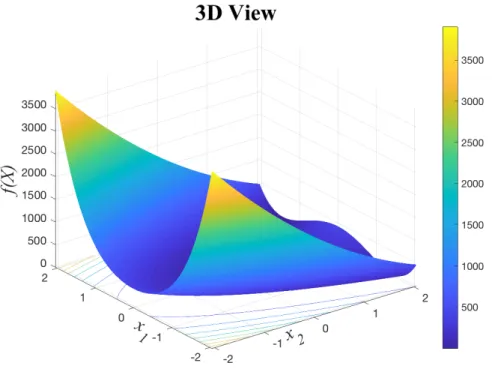
5.1.7 Generalized Rosenbrock’s Valley

f(X) = n−1

∑

i=1 h 100 x_i+1−x2i 2 + (x_i−1)2 i (22) The Generalized Rosenbrock’s Valley (also known as Rosenbrock’s Banana Function, or The 2nd De Jong’s Function) is the final generalized function we use for testing.

Rosenbrock is perhaps unique in our testing benchmarks. The function’s optimal point is lo-cated in a narrow, parabolic valley. Forn=2,3, this function only has one minimum. Forn=4−7, there are exactly 2 minima (one being local and the other global), and the number is unknown for highern.

What makes Rosenbrock a particularly interesting function to test with is that despite having no local minima in the search region, this function is nevertheless surprisingly difficult to optimize. The parabolic valley in which the global minimum resides is demonstrably very “easy” for an opti-mization algorithm to converge to. However, converging upon the global minimum after reaching

(31)

this valley is difficult. Essentially, one may think of it as testing for an opposite extreme case as Griewank and Ackley.

Figure 9: 3-dimensional rendering of Rosenbrock’s Banana Function withn=2

Our overall combination of these 7 different testing functions provides a significant range of different challenges to better discern specific function behaviors and determine the usefulness and performance of our GEM-PSO variants.

(32)

6

Results

In this section we detail our data collection process, as well as our results, broken down by single parameter variation performance, isolated modification performance, and combined modifi-cation performance, across different PSO parameters, memory size, and function. Single parameter variation refers to the parameters of the standard PSO algorithm, such as dimension of the function to optimize, population of the swarm, and the neighborhood type of the swarm. In the isolated modification section, we look at GEM-PSO variants with only one deviation from the standard-PSO algorithm, i.e. only one adding or one selecting or one removing modification. Finally, the combined modification performance covers our GEM-PSO variants with multiple modifications applied at the same time.

6.1

Early Testing and Filtering Techniques

Preliminary testing indicated that applying modified improvements to both personal and neigh-borhood bests strongly hindered convergence to the point that most runs on any arbitrary combina-tion of PSO parameters and funccombina-tions ended up diverging. Therefore, we limited our early testing methodology to varying only personal or neighborhood past best utilization methods.

We performed 30 runs of every combination of adding, selection, and removal mechanism applied to either neighborhood or personal combinations, crossed our varied parameters for di-mension, swarm population, function number, and neighborhood type, as well as the number of past bests to save. Iterations was fixed at 1000, as the nature of the functions we were working with guaranteed that this was more than sufficient for convergence to take place for standard PSO, and though a worse-performing modified algorithm may not converge as quickly, we were interested in finding modifications that improved behavior (so a function that did not manage to converge within 1000 iterations was likely to be an unsuitable combination). Our total number of unique settings is therefore

30×3×4×4×2×2×7×3×3=362880.

We wanted to perform a per-100 iteration statistical and numerical analysis on the best-performing modification combinations. This would be far more costly than our preliminary testing in terms of both space and time requirements, so we needed to filter the viable combinations down much further from this initial quantity. The simplest filtration we could perform was to take a baseline PSO solution average for each given combination of PSO parameters (with no personal or neigh-borhood modifications). We call this value s_base, and filtered all solutions by checking, for each combination of modifications, whether there was at least one occurrence of a solution (call it s2)

which satisfied

s₂<(s_base+1)∗10.

This eliminated all solutions that were beyond an order of magnitude worse than the baseline regular PSO, and also accounted for instances where the solution’s order of magnitude could be very small (for instance, in sphere, directly checking for an order of magnitude would require solutions better than 0.00001, which we decided was overly strict).

(33)

After the elimination process for personal modifications and neighborhood modifications, we were left with only 14 viable personal modifications and 14 (not the same) viable neighborhood modification combinations, down from the original 32 possible combinations. We use the enumer-ated modifications (Table 5) to concisely list the viable combinations.

Personal [010] [012] [020] [022] [030] [031] [032]

[110] [112] [120] [122] [130] [131] [132]

Neighborhood [020] [021] [022] [023] [030] [032] [033]

[120] [121] [122] [123] [130] [132] [133]

Table 3: Combinations Passing First Filter

One may notice that these are not the same 14 combinations. However, this initial filtering is not sufficient to guarantee our remaining modification combinations are worth further exploring. It is enough of a reduction in quantity, though, to apply more detailed analysis.

We then performed testing of 10 runs (recording the solution quality at each 100 iterations) for each remaining personal or neighborhood modification (varying all PSO parameters as before), along with 10 runs of a benchmark with the same PSO parameters, computed a Mann-Whitney U Test and a Student T Distribution Test on each 100 iterations’ data. Using a p-value cutoff of 0.05, we performed one last filtration of data by requiring either the p-value found by Mann-Whitney or the t-test to be above 0.05 for at least one combination of PSO parameters, or for the average solution quality to be better than the benchmark solution average. After this final filter, we were left with exactly 11 personal modification combinations and only 6 viable neighborhood modification combinations, allowing us to concentrate on this data.

Personal [0, 1, 0] [0, 1, 2] [0, 2, 0] [0, 2, 2] [0, 3, 0] [0, 3, 2]

[1, 1, 0] [1, 2, 0] [1, 2, 2] [1, 3, 0] [1, 3, 2]

Neighborhood [0, 2, 0] [0, 2, 2] [0, 2, 3] [0, 3, 0] [0, 3, 2] [0, 3, 3]

Table 4: Combinations Passing Second Filter

Here we re-print the legend of enumeration corresponding to different modifications for ease of understanding.

Adding/Saving Replacing/Removing Selecting/Using

0 - Save Best (Standard) 0 - Replace Oldest 0 - Select Best (standard)

1 - Save with Probability 1 - Replaced Last-Used 1 - Select Random

2 - Save with Distance Metric 2 - Replace Worst (standard) 2 - Select 2 Past Bests

with Equal Weighting

3 - Replace Random 3 - Select with

Tournament Selection

(34)

It is worth noting that in this final set of possible modification combinations that not a single combination utilizing replace-oldest (removing the earliest-found past best), in either personal or neighborhood modifications, was able to pass our defined filter, which strongly suggests that, similar to save-distance, this modification is likely to decrease performance quality. Therefore, it should be discarded.

This process of filtering, performing more detailed analysis, filtering again, and using the fi-nal viable data was a key component of our ability to conduct enough testing runs to verify that any behavior we noticed was statistically significant and that we could be reasonably certain our modifications were at least not statistically worse than the benchmark PSO.

As an additional point of interest, we computed the frequency with which a modification com-bination (averaged over 10 runs) yielded a better result than the benchmark PSO. The frequencies of these calculations are presented in the tables below.

Modifications (Personal) Frequency of Best Performance

Save with Probability,

Select with Equal Weighting 8

Replace Randomly,

Save with Probability,

Replace Last Used 9

Replace Randomly 4

(No Modifications) 21

Save with Probability 7

Save with Probability, Replace Randomly, Select with Equal Weighting

2

Replace Last Used 5

Table 6: Personal Modifications Frequency

Modifications (Neighborhood) Frequency of Best Performance

(No Modifications) 30

Select with Tournament Selection 30

Replace Randomly 1

Table 7: Neighborhood Modifications Frequency

From these tables, it is reasonable to conclude that these modifications hold significant poten-tial. At the very least, it establishes that the standard, benchmark PSO does not directly outperform all possible modifications we have created.

(35)

6.2

Impact of PSO Parameters

First, we observe the general impact of PSO’s parameters on the performance of our GEM-PSO variants.

6.2.1 Dimension and Population

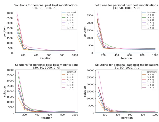
Extensive comparison of PSO performance across dimension and population shows that the performance of each algorithm is relatively consistent across all 4 combinations (30 or 50 dimen-sions in the test function, and 30 or 50 particles in the swarm).

The graphs below demonstrate selected examples of this consistency of behavior across dif-ferent functions. Figure 10 shows personal modification PSOs run on Rosenbrock, and Figure 11 shows neighborhood modification PSOs run on Rastrigin.

Figure 10: Dimension and Population Combinations for Personal-Modified PSO, 4 Past Bests, in Rosen-brock

(36)

Figure 11: Dimension and Population Combinations for Neighborhood-Modified PSO, 4 Past Bests, in Rastrigin

The [a,b,c,d,e] subtitle labels are created because of space constraints. These can be in-terpreted as [dimension, population, total number of iterations, function number, neighborhood type]. The function numbers and neighborhood numbers can be found in Table 9 and Table 10, respectively.

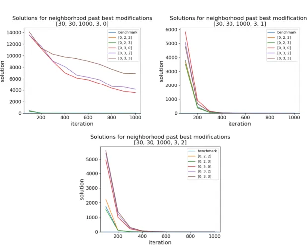
One may notice that three of the neighborhood PSO modifications seem to not be converging on even a near-optimal solution. Specifically, the modifications [0, 3, 0], [0, 3, 2], and [0, 3, 3] exhibit this undesirable behavior. They share in common the modification replace-random, and it turns out this observed behavior in our neighborhood modifications can be directly attributed to replace-random’s influence. We will discuss replace-random in a separate section about the impact of specific, isolated modifications on GEM-PSO performance.

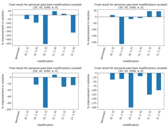
The consistency in each algorithm’s behavior across dimensions persists across different neigh-borhood types, different functions, and even whether the modifications are applied to personal or neighborhood components in the algorithm. However, it is important to note that there exists an exception, when using 50 dimensions and 50 particles, in the relative performance between bench-mark PSO and GEM-PSO variants. For example, consider this diagram, which shows personal-modified PSOs run on Penalized Function No. 01. Standard PSO tends to perform decently but

(37)

does yield significantly superior results to other modified PSOsexceptwhen using 50 dimensions and 50 particles.

Figure 12: Dimension and Population Combinations for Personal-Modified PSO, 4 Past Bests

As one can see from Figure 12, when using 50 dimensions and 50 population size, standard PSO performs significantly better than the other modifications, while it does not do so for every other tested combination of dimension and population. This supports our analysis that while the impact of dimension and population on the performance of our GEM-PSO variants is similar to its impact on standard PSO, the magnitude of the impact may be greater on our variants, which results in standard PSO’s better performance on this specific setting.

We believe that the consistency and frequency of this behavior suggests that standard PSO may scale more effectively when matching dimensions to particle size. However, one would need to construct many additional tests to fully understand the underlying cause for this behavior, and this falls outside the scope of our study.

6.2.2 Neighborhood Type

We know that the performance of standard PSO is quite different when applied to different functions (simply because convergence and exploration are highly dependent upon function topol-ogy), and our GEM-PSO algorithms are no different. It is more reasonable to compare the dif-ference in performance between GEM-PSO variants held constant in all parameters except for

(38)

neighborhood topology. The figures below demonstrate the effect of neighborhood topology, us-ing a representative figure with personal-modified GEM-PSO variants applied to Griewank and Rosenbrock, with 4 past best memory.

Figure 13: Varying Neighborhood Topologies for Personal-Modified PSO, 4 Past Bests, on Griewank

(39)

In order from left to right, top to bottom, we have Global, Ring, and Von Neumann neighbor-hoods, for both sets of diagrams. One may note some variation (Global converges fastest, followed by Von Neumann, and finally Ring topology), but we can see the influence of neighborhood topol-ogy on the performance of our GEM-PSO variants is quite similar to its influence on standard PSO (as shown by the variation on the benchmark line). This is an expected behavior - neigh-borhood topology doesn’t have nearly as much impact on our modifications here because these modifications are only applied to the personal influence component.

This of course raises the question: what is the influence of neighborhood topology on our based modifications? Below are graphs demonstrating this effect, applied to neighborhood-modified GEM-PSO variants, tested on Griewank and Rosenbrock, holding all other parameters constant.

(40)

Figure 16: Varying Neighborhood Topologies for Neighborhood-Modified PSO, 4 Past Bests, on Rosen-brock

Now we see a far more striking impact. When using global neighborhoods, some of our GEM-PSO variants completely fail to converge within 1000 iterations (if we were to let the program continue to run, it is possible judging by the graph that convergence could be achieved, but would take far too many iterations to be viable). Those same swarms converge (although still too slowly to be comparable to the three swarms on par with benchmark) when using Von Neumann neigh-borhood topology, and converge far more quickly when using Ring topology. However, the better these two swarms perform, the worse the other 3 swarms perform. This behavior can be attributed to a fundamental difference our modification has introduced - with the 3 successful swarms (stan-dard PSO, [0, 2, 2], [0, 2, 3]), introducing more past bests increases the neighborhood best solution fitness, because they share the remove-worst feature. The more particles are in a neighborhood, the more likely the solution quality is greater. The greater level of exploitation thus directly translates to faster convergence. On the other hand, the two swarms that fail to converge ([0, 3, 0] and [0, 3, 3]) use replace-random. The more particles are in a neighborhood, the more dilute and random the

neighborhood best becomes. And therefore,nbest introduces more exploration, which depending

on the neighborhood size, can hinder convergence too strongly. These functions therefore exhibit this opposite behavior we observed.

(41)

6.3

Isolated Modifications

Let’s observe our results for GEM-PSO variants with single modifications (i.e. only changing one of our 3 different modification types).

6.3.1 Personal Modifications

After our two levels of filtering, we are left with 4 GEM-PSO variants that use a single mod-ification. They are [0, 3, 0], [0, 2, 2], [1, 2, 0], and [0, 1, 0], corresponding to replace-random, select-equal-weighting, save-probability, and replace-last-used, respectively.

Let’s look at save-probability versus save-best (benchmark). Extensive testing (example graphs done with Rastrigin for consistency below) demonstrates that save-probability performs better with fewer past-bests.

Figure 17: Varying Neighborhood Topologies for [1, 2, 0] , 2 Past Bests

No discernable difference was found for varying the number of past bests saved (which is a reasonable behavior given we are selecting the past best with the highest fitness, meaning that more, likely less fit past bests will not influence our algorithm). However, to draw distinct conclusions about save-probability’s impact on performance, we refer to a different kind of graph, a line-plot

(42)

of Mann-Whitney tests performed at each 100 iterations on 10 independent solutions generated by benchmark and our GEM-PSO.

Figure 18: Mann-Whitney Analysis of [1, 2, 0] on Rastrigin, 3 Past Bests

We can see from the graph on the left a significant improvement (roughly by 100 units of solu-tion quality), but because this is an average of 10 values, the argument could be made that this may not be a significant improvement, or could be due to natural variation from a stochastic algorithm. Once we apply Mann-Whitney U Test, however, it becomes clear that our [1, 2, 0] function’s results are significantly different from the behavior of standard PSO, and therefore represents a significant improvement.

Because these behaviors are most strongly observed when using Ring topology, a neighborhood that is small (size 2) and therefore less computationally expensive to maintain, this function would be more desirable/better applied in scenarios where neighborhood computations are costly and ideally avoided as much as possible.

Now we analyze [0, 2, 2], corresponding to select-equal-weighting. This is a very promising modification to PSO, as judging by our frequency lists from earlier, this PSO was the best PSO possible for more different parameters than standard PSO was. In essence, it has potential to either outperform standard PSO in specific, specialized cases, or it could be a generally better-performing algorithm.

Preliminary testing shows that this modification exhibits some of the same behaviors as [1, 2, 0], such as being optimal under Ring topology, and generally performs better under smaller past-best memory. It consistently outperforms standard PSO on Griewank and Sphere, and performs almost exactly the same on Rosenbrock. These figures demonstrate performance and statistical significant with 2 past best memory.

(43)

Figure 19: Mann-Whitney Analysis of [0, 2, 2] on Griewank

Figure 20: Mann-Whitney Analysis of [0, 2, 2] on Sphere

(44)

Applied to Griewank, the algorithm improves sharply (to a point where at 400-700 iterations it performs