A Self-Improving Convolution Neural Network for
the Classification of Hyperspectral Data
Pedram Ghamisi,
Member, IEEE,
Yushi Chen,
Member, IEEE,
Xiao Xiang Zhu,
Senior Member, IEEE
Abstract—In this paper, a self-improving convolutional neural network (CNN)-based method is proposed for the classification of hyperspectral data. This approach solves the so-called curse of dimensionality and the lack of available training samples by iteratively selecting the most informative bands suitable for the designed network via fractional order Darwinian particle swarm optimization (FODPSO). The selected bands, then, are fed to the classification system to produce the final classification map. Experimental results have been conducted with two well-known hyperspectral data sets; Indian Pines and Pavia University. Re-sults indicate that the proposed approach significantly improves a CNN-based classification method in terms of classification accuracy. In addition, this paper uses the concept ofditherfor the first time in the remote sensing community to tackle overfitting.
Index Terms—Hyperspectram image classification, Deep
Learning, CNN, Feature Selection, FODPSO.
I. INTRODUCTION
C
OMPLEX light scattering mechanisms in naturalob-jects (e.g., vegetation), different atmospheric scattering conditions, and intra-class variability make the hyperspectral imaging process inherently nonlinear. It is believed that deep architectures can lead to progressively more abstract features at higher layers of features, and more abstract features are generally invariant to most local changes of the input.
Deep learning is characterized by the so-called “deep” neural network (DNN) architectures, i.e., deeper than three layers. If designed and trained properly, a DNN provides a hierarchical description of the input data in terms of relevant and easy to interpret features at every layers.
Depending on the architecture and the involved activation functions, several classes of DNNs have been developed such as: deep belief networks (DBN) [1], deep Boltzmann machines (DBM) [2], and autoencoders (AE) [3]. The use of deep learning for hyperspectral image analysis is still in its beginning period and the number of research works in this field is very limited. In [4], a stacked AE-based approach was introduced for hyperspectral data classification. In [5], a DBN-based feature extraction was proposed for the classification of hyperspectral data. In those approaches, however, there is a full connection between different layers and consequently, they Pedram Ghamisi and Xiao Xiang Zhu are with German Aerospace Cen-ter (DLR), Remote Sensing Technology Institute (IMF) and Technische Universit¨at M¨unchen (TUM), Signal Processing in Earth Observation, Mu-nich, Germany (corresponding authors, e-mail: [email protected] and [email protected]).
Yushi Chen is with the Department of Information Engineering, Harbin Institute of Technology. (e-mail: [email protected]).
This research has been partly supported by Alexander von Humboldt Fellowship for postdoctoral researchers, and Helmholtz Young Investigators Group “SiPEO” (VH-NG-1018, www.sipeo.bgu.tum.de).
demand to train a lot of parameters, which is an undesirable factor due to the lack of available training samples.
Among deep approaches, CNNs have attracted many re-searchers since they use local connections to handle spatial dependencies. In addition, CNNs share weights which sig-nificantly deceases the number of parameters needed to be trained in comparison with other deep approaches. However, the number of parameters is still high when one needs to deal with hyperspectral data. Inappropriate weights may cause getting trapped in a local minimal of the loss function. To obtain proper weights, a lot of training samples are needed for the training procedure. However, the number of available training samples is usually limited, which downgrades the result of most supervised learning approaches. Recently, few regularization methods have been introduced in order to deal with overfitting problems including L2 regularization and dropout [6]. Due to the high spectral dimensionality and the limited training samples in hyperspectral data, however, the existing regularization methods cannot handle the overfitting problem properly.
To address the issue of imbalance between dimensionality and the number of available training samples, different feature selection approaches can be considered. Conventional feature selection techniques usually demand many samples in order to accurately estimate statistics [7]. Moreover, most of those approaches are based on exhaustive search to find the best set of features among the whole dimensionality, which requires a huge CPU processing time and many RAMs in order to successfully lead to a conclusion [7]. To address the aforemen-tioned issues, the new trend for feature selection is based on
evolutionary-based optimization approaches, such as genetic
algorithm (GA) andParticle Swarm Optimization(PSO) [8].
For example in [9], a GA was used to regulate hyperplane parameters of an SVM, while it finds efficient features to be fed to the classifier.
PSO has a simple concept, which can be implemented in a few lines of code. Moreover, PSO has a memory of past iterations. However, the main disadvantage of PSO is the premature convergence of the swarm. The main reasons of this disadvantage are: (i) particles try to converge to a single point, which is located on a line between the global best and the personal best positions. This point, however, is not guaranteed to be a local optimum [7], and (ii) the fast rate of information flow between particles leads to the creation of similar particles, which results in a loss in diversity. In [10], an algorithm was proposed for feature selection based on fractional order Darwinian particle swarm optimization (FODPSO) to address the main shortcoming of the PSO, i.e.,
the premature convergence of a swarm.
This paper proposes a classification approach, here entitled as self-improving CNN (SICNN), which is based on con-sidering FODPSO as feature selection, and the classification accuracy of CNN on validation samples as fitness value. The proposed approach addresses the main shortcoming of a CNN-based classification approach for hyperspectral data, i.e., the lack of available training samples, by automatically selecting the best set of bands from the whole dimensionality suitable for the defined network. The proposed approach is applied to Indian Pines and Pavia University using the standard training and test samples. It should be noted that, in this paper, feature selection has been used for the first time to improve the capability of deep networks in the hyperspectral community.
In addition, this paper considers the concept of dither[11] as
a regularization method for the first time in the remote sensing community to further address the issue of overfitting for CNN. The rest of the paper is organized as follows: Section II introduces the methodology of the paper. Section III is devoted to experimental results. The main concluding remarks are mentioned in Section IV.
II. METHODOLOGY
We believe that there are two possible ways to cope with deep approaches for the classification of hyperspectral data: (1) one can experimentally modify the architecture of the network and set the parameters in a trial and error way, which is, of course, time demanding. It is easy to understand that the network defined in this way needs to be changed from one data to another and from one set of training samples to another one due to the lack of generalization. (2) One can define a fix yet logical network and define the most suitable bands based on the network. This paper follows the second possible way.
Fig. 1 depicts the main work flow of the proposed approach. In this paper, the performance of the CNN is improved via an FODPSO-based feature selection. In more detail, the overall accuracy (OA) of CNN on validation samples is improved toward the optimization process by iteratively selecting the most informative features in terms of the OA. Finally, a CNN is applied to the selected bands and the obtained result is eval-uated on the test samples. In the following sections, FODPSO-based feature selection and CNN-FODPSO-based classification, which are the backbones of SICNN, will be elaborated on.
CNNs have a unique architecture in comparison with other deep models by using local connections and shared weights. In CNN, some connections between neurons are replicated across the entire layer, which share the same weights and
biases.1 A deep CNN is composed of several convolutional
and pooling layers to form a deep architecture followed by a fully connected logistic regression (LR) layer at the end. We first define the convolutional layer as follows:
xlj =f M X i=1 xli−1∗klij+blj ! , (1)
1It should be noted that the concept of end-to-end training has been recently
introduced to obtain deeper networks and have fewer parameters to be trained to further improve the ability of CNNs.
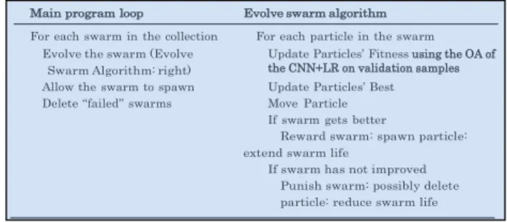
Self-Improving CNN
(1) Split the training set to two sets: training and validation (2) Run FODPSO with CNN+LR as the corresponding fitness criterion as follows until the maximum number of iterations is met.
Main program loop Evolve swarm algorithm For each swarm in the collection For each particle in the swarm
Evolve the swarm (Evolve Swarm Algorithm: right)
Update Particles’ Fitness using the OA of the CNN+LR on validation samples Allow the swarm to spawn Update Particles’ Best
Delete ‘‘failed’’ swarms Move Particle If swarm gets better
Reward swarm: spawn particle: extend swarm life
If swarm has not improved Punish swarm: possibly delete particle: reduce swarm life (3) Choose the best particle with the highest fitness as the output (4) Use the whole training set to train CNN+LR on the selected bands from (3).
(5) Evaluate the final classification results using test samples.
Fig. 1. The general idea of the SICNN.
where xli−1 represents the i-th feature map of (l-1)-th layer.
xl
j is the j-th feature map of the current (l)-th layer, and M
denotes the number of input feature maps. kl
ij and blj are
the trainable parameters in the convolutional layer. f(.) is a
nonlinear function and∗ is the convolution operation.
Pooling can extract invariant features by reducing the reso-lution of feature maps. Each pooling layer corresponds to the
previous convolutional layer, while it combines a smallN×1
patch of the convolution layer. The most common pooling technique is max pooling.
To handle the issue of overfitting to some extent, we
have considereddropout, and to accelerate the convergence, a
rectified linear unit(ReLU) is used. There are different types of ReLUs to be considered in the network. In this study, a simple nonlinear ReLU operation was considered, which accepts the input of a neuron if it is positive, while it returns 0 if the input is negative. Dropout sets the output of some hidden neurons to zero, and the dropped neurons do not contribute in the forward pass as well as the back propagation procedure. At different training epochs, the deep CNN introduces different neural networks by dropping neurons in a random way. By using ReLU and dropout, the outputs of many neurons turn to 0. The consideration of the ReLU and dropout at several layers build up a powerful sparse-based regularization for the deep network and address the overfitting problem for hyperspectral image classification.
In nonlinear signal processing, the use of additive noise prior to nonlinear processing can decorrelate nonlinear
dis-tortion products. Such process is regarded as dithering. In
this context, DNNs can be considered as discrete (sampled) systems composing of linear filters and nonlinear demodu-lation stages. As mentioned in [12], the so-called inherent nonlinear distortion and aliasing lead to the issue of overfitting. Therefore, if dither can suppress nonlinear distortion and aliasing, it might also be a useful tool to regularize the CNN. As a result, to further mitigate the issue of overfitting, in
addition to dropout, we introduce a simple yet effective method
named dither, based on [11], to improve the regularization
procedure. New sample ym is obtained by adding random
noise to a training sample xm as ym = xm+βn, in which
n is the additive noise, while β controls the intensity of the
random Gaussian noise n.
In this paper, the output of CNN is classified using an LR, which employs soft-max as its output-layer activation. Soft-max ensures the activation of each output unit sums to one. Therefore, the output can be seen as a set of conditional
probabilities. Given the input vectorR, the probability that the
input sample belongs to class iis estimated as follows:
P(Y =i|R, W, b) =s(W R+b) = e WiR+bi
P
jeWjR+bj
(2)
where W and b are weights and biases of the LR layer,
respectively, while the summation is done over all the output units. LR can be considered as a single layer neural network and as a result, it can be merged with the CNN to form a CNN+LR deep classifier. In this manner, the size of the output-layer should be equal to the number of classes.
A. FODPSO-based Feature Selection
FODPSO was proposed in [13] for image segmentation. FODPSO can overcome the main drawback of a simple PSO, i.e., the stagnation of particles around sub-optimal solutions by considering two main modifications:
1) FODPSO run many simultaneous parallel PSO algo-rithms, each one as a different swarm, on the same test problem and then a simple natural selection mechanism is applied. When a search tends to a sub-optimal so-lution, the search in that area is simply discarded and another area is searched instead. In this approach, at each step, swarms that get better are rewarded (extend particle life or spawn a new descendent) and swarms that stagnate are punished (reduce swarm life or delete particles). For more information, please see [13]. 2) Fractional calculus is used to control the convergence
rate of the algorithm. This method has been further in-vestigated for image segmentation and feature selection in [10, 13]. The main advantage of fractional calculus is that while an integer-order derivative just implies a finite series, the fractional-order derivative requires an infinite number of terms. More precisely, integer derivatives are “local” operators, while fractional derivatives have, implicitly, a “memory” of all past events, which is useful to control the dynamic of each swarm.
For detailed information about the FODPSO-based feature selection please see [10]. In order to consider the concept of the FODPSO for feature selection, the following points need to be considered:
1) The dimension of each particle should be equal to the number of bands. Therefore, the velocity dimension (dim
vn[t]), as well as the position dimension (dim xn[t]), at
iterationt, are equal to the total number of bands of the
hyperspectral image, i.e.,dim vn[t] =dim xn[t] =l.
2) Since FODPSO is used here for band selection, each particle should be represented its position in binary val-ues, in which 0 shows the absence of the corresponding band, while 1 shows the presence of the corresponding band. In this case, as mentioned in [10], the velocity of a particle can be considered as a probability to change the binary value from 0 to 1 or vice versa. In order to obtain a binary position, one can, first, normalize velocities in the range of 0 and 1 as follows:
∆xn[t+ 1] =
1
1 +e−vn[t+1] (3) Consequently, the position of each particle can be rep-resented as follows: xn[t+ 1] = ( 1, ∆xn[t+ 1]≥r 0, ∆xn[t+ 1]< r (4)
wherein r is a random l-dimension vector with each
component generally a uniform random number between 0 and 1.
3) The OA of CNN+LR on validation samples can be considered as the fitness value.
III. EXPERIMENTAL RESULTS
In this paper, two widely used hyperspectral data have been used. The first data set (Indian Pines) was captured by AVIRIS over a rural area in NW Indiana. For this data set, 200 data channels are used after the removal of the spectral bands affected by atmospheric absorption. The second data set (Pavia University) is of the Engineering School at the University of Pavia captured by ROSIS-03. In the experiments, 12 noisy data channels are eliminated, and 103 data channels are used for processing. We intentionally selected these two data sets since they are different in many aspects such as spatial resolution, number of bands and the type of the scene and land-covers, which can be useful to evaluate the generalization capability of the proposed method.
In order to evaluate the capability of SICNN in an ill-posed situation (i.e., when there is no balance between the number of training samples and bands), and make the approach fully comparable with the-state-of-the-arts, for both data sets, the standard sets of training and test samples have been taken into account. For detailed information about the data sets and their corresponding test and training samples, please see [14]. The total number of training and test samples for Indian Pines are 695 and 9671, respectively, while for Pavia University are 3912 and 42776, respectively.
Deep learning uses deep neural networks, which are in-herently parallel algorithms. To accelerate the training time, “matconvnet-1.0-beta18” with CUDA configuration is adapted. In order to keep the borders of different features through convolutional layers, the original image is padded with an extra artificial border, which mirrors the original border.
In this work, 90% of the training samples have been used to train weights and biases and the rest as validation samples to guide the design of a proper architecture in order to avoid overfiting. It should be noted that the validation samples are
different from the test samples. The validation samples have been extracted directly from the training set.
In this paper, we only included the classification accuracy of the SVM and RF (as two strong classifiers to handle high dimensional data with a limited number of training samples [7]) to show that the proposed method is also capable of handling ill-posed situations, while a direct comparison of these approaches with SICNN is not expected. For the SVM, an RBF kernel is taken into account and the hyperplane parameters have been adjusted via five-fold cross validation. The number of trees for RF is set to 200. For the FODPSO, we used the same set of parameters as [10].
The input hyperspectral data sets were normalized in the
range of [−0.5 0.5]. To exploit sufficient spatial information
for the pixel to be classified, a large patch with the size of
27×27was used. Since the studied areas are of small sizes,
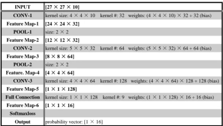
only three convolution layers and two pooling layers have been used. Details of the architecture for the CNN are listed in Fig. 2. It should be noted that the same network has been used for both data sets.
In the training procedure, a mini batch with a size of 32 was used. For relatively small training samples, as in our case, this could allow the training step to perform more frequent parameter updates and achieve faster convergence in practice. In addition, a dynamic learning rate is adopted in our case. The whole training period is divided into five stages, starting from a learning rate of 0.01, and decreasing by half for the subsequent stage. This setting provides a fast descend of loss function at the beginning, while the gradual decreasing rate can ensure a small but consistent progress. After reaching a certain stage of training, a big rate may no longer be suitable since it causes oversteps and gives a higher loss. This way of adjusting the learning rate enables the algorithm to be converged in a very few iterations. For Indian Pines, the inner number of iterations (CNN as the fitness metric for feature selection) is set to 20 while the outer number of iteration (for the final classification of the selected bands) is set to 80. For Pavia University, the inner and outer numbers of iterations are set to 10 and 20, respectively. The difference between the inner and outer number of iterations is due to the fact that the number of training samples for the inner feature selection is significantly fewer than the ones for the outer classification step. Hence, the number of demanded iterations is also lower. The reason why the number of iterations is different for Indian Pines and Pavia University lies on the differences between the data sets, i.e., the number of bands and classes.
In this paper, RF, SVM, andCNN+LR refer to situations
where the input data sets are classified by RF, SVM, and
CNN+LR respectively. SICNNdither and SICNN represent
the performance of the proposed approach, with and without dither, respectively.
A. Experimental Results
The obtained classification accuracies for both data sets have been reported in Table I. The results show that the proposed
SICNN can improve the classification accuracy ofCNN+LR,
RF, andSVM in almost all situations. The only exception is
INPUT CONV-1 Feature Map-1 POOL-1 Feature Map-2 CONV-2 Feature Map-3 POOL-2 Feature. Map-4 CONV-3 Feature Map-5 Full Connection Feature Map-6 Softmaxloss Output [27 × 27 × 10]
kernel size: 4 × 4 × 10 kernel #: 32 weights: (4 × 4 × 10) × 32 + 32 (bias) [24 × 24 × 32]
size: 2 × 2 [12 × 12 × 32]
kernel size: 5 × 5 × 32 kernel #: 64 weights: (5 × 5 × 32) × 64 + 64 (bias) [8 × 8 × 64]
size: 2 × 2 [4 × 4 × 64]
kernel size: 4 × 4 × 64 kernel #: 128 weights: (4 × 4 × 64) × 128 + 128 (bias) [1 × 1 × 128]
kernel size: 1 × 1 × 128 kernel #: 9 weights: (1 × 1 × 128) × 16 + 16 (bias) [1 × 1 × 16]
probability vector: [1 × 16]
Fig. 2. Detailed information about the network considered for CNN and SICNN. 10 20 30 40 50 60 70 80 90 100 Run 5 OA = 84.41% 20 40 60 80 100 120 140 160 180 200 Run 8 OA = 84.21%
Fig. 3. Selected bands by the proposed approach usingdither; from top to bottom: the fifth run on Pavia University and the eight run on Indian Pines.
that SVM yields the best AA compared to other approaches
for Pavia University.
According to Table I, in most cases, the SVM can
out-perform the CNN+LR. The reason is that for SVMs, in
order to train the classifier, only samples that are close to the class boundary (support vectors) are needed to locate the hyperplane vector in the feature space. Therefore, SVMs can efficiently handle high dimensional data with a limited number of training samples. However, the CNN needs to train a huge number of parameters and consequently, many training samples are demanded. With reference to Table I, this problem can be addressed to a great extent using the proposed approach combined by the FODPSO. In more detail, the FODPSO can iteratively selects the most appropriate set of bands suitable for the network.
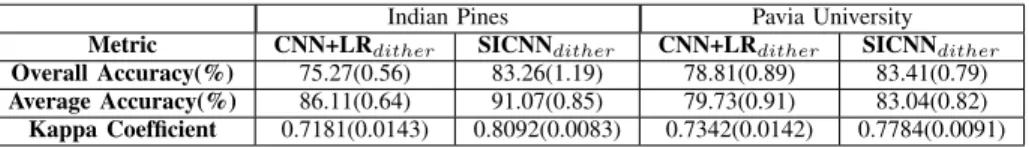
Table II gives information about classification accuracies
obtained by CNN+LR and SICNN with the dither. With
reference to Tables I and II, one can notice an improvement in terms of classification accuracy using this regularization approach. The main reason of this improvement is that dither
helps the CNN+LR and SICNN to tackle overfitting and
be converged quickly. As mentioned, the inner number of iterations for Indian Pines and Pavia are set to 20 and 10, respectively. However, this numbers might not be enough to guarantee the convergence of each swarm appropriately. Dither leads to a fast learning and convergence, which is beneficial for the proposed approach. Fig. 3 demonstrates the sets of bands with the highest OA among 10 runs selected by the
proposed approachSICNNdither. The OA of each set is also
shown in the figure. The number of selected bands for Pavia University and Indian Pines are 22 and 55, respectively.
IV. CONCLUSION
In this paper, a self-improving hyperspectral classification approach is proposed, which is based on a deep CNN and
TABLE I
CLASSIFICATION ACCURACIES OF DIFFERENT APPROACHES INCLUDING: RF, SVM, CNN+LRANDSICNNFOR BOTHINDIANPINES ANDPAVIA UNIVERSITY. THE BEST RESULT IS SHOWN IN BOLD TYPE FACE. FORCNN+LRANDSICNN,THE AVERAGE VALUES OF10RUNS ARE REPORTED AND
THE STANDARD DEVIATION OF THE RUNS HAVE BEEN SHOWN IN BRACKETS.
Indian Pines Pavia University
Metric SVM RF CNN+LR SICNN SVM RF CNN+LR SICNN
Overall Accuracy(%) 78.20 70.24 74.44(0.81) 81.66(1.70) 78.21 71.64 78.45(1.04) 82.67(1.27)
Average Accuracy(%) 86.00 76.98 85.39(0.58) 89.64(1.11) 87.14 82.25 79.05(0.67) 82.18(0.59)
Kappa Coefficient 0.75 0.6642 0.7123(0.0093) 0.7933(0.0165) 0.7333 0.6511 0.7312(0.0093) 0.7716(0.0156)
TABLE II
THE SIGNIFICANCE OF USING DITHER ON CLASSIFICATION ACCRACIES. Indian Pines Pavia University
Metric CNN+LRdither SICNNdither CNN+LRdither SICNNdither
Overall Accuracy(%) 75.27(0.56) 83.26(1.19) 78.81(0.89) 83.41(0.79)
Average Accuracy(%) 86.11(0.64) 91.07(0.85) 79.73(0.91) 83.04(0.82)
Kappa Coefficient 0.7181(0.0143) 0.8092(0.0083) 0.7342(0.0142) 0.7784(0.0091)
FODPSO. In this approach, we let the CNN find the most informative bands from the existing ones using the FODPSO-based feature selection. The overall accuracy of CNN+LR on validation samples was considered as fitness value. Based on obtained fitness values on validation samples, FODPSO iter-atively tries to eliminate extra bands by considering many si-multaneous parallel PSO algorithms, some specific punishment and reward rules, and using the concept of fractional calculus to model the dynamic of the swarm. Results indicate that the SICNN can significantly improve the CNN+LR in terms of classification accuracies and can classify hyperspectral data when there are only a limited number of training samples are available. In addition, in this paper, the concept of dither was proposed to efficiently regularize CNNs to improve the classification performance of the proposed method.
Both CNN and SICNN extracts spatial information using a fixed neighborhood system. In order to improve the classifica-tion accuracy, one can consider adaptive neighborhood system-based approaches such as morphological profile, attribute profiles, and segmentation approaches.
V. ACKNOWLEDGMENT
The authors would like to sincerely appreciate Prof. Paolo Gamba from the University of Pavia, Italy and Prof. David Landgrebe from Purdue University to provide Pavia University and Indian Pines data sets, respectively.
REFERENCES
[1] G. E. Hinton, S. Osindero, and Y. Teh, “A fast learning
algorithm for deep belief nets,” Neural Comp., vol. 18,
no. 7, pp. 1527–1554, 2006.
[2] R. Salakhutdinov and G. E. Hinton, “Deep boltzmann
machines,” Int. Conf. Art. Intel. Stat., pp. 448–455,
Clearwater Beach, Florida, 2009.
[3] Y. Bengio, P. Lamblin, D. Popovici, and H. Larochelle,
“Greedy layer-wise training of deep networks,” Neural
Inf. Proc. Sys. 19, pp. 153–160, Cambridge, USA, 2007. [4] Y. Chen, Z. Lin, X. Zhao, G. Wang, and Y. Gu, “Deep
learning-based classification of hyperspectral data,”IEEE
Jour. Sel. Top. App. Earth Obs. Remote Sens., vol. 7, no. 6, pp. 2094 – 2107, 2014.
[5] Y. Chen, X. Zhao, and X. Jia, “Spectra-spatial classifica-tion of hyperspectral data based on deep belief network,” IEEE Jour. Sel. Top. App. Earth Obs. Remote Sens., vol. 8, no. 6, pp. 2381–2292, 2015.
[6] A. Krizhevsky, I. Sutskever, and G. E. Hinton, “Imagenet classification with deep convolutional neural networks,” Proc. Adv. Neural Inf. Process, pp. 1097 –1105, 2012.
[7] J. A. Benediktsson and P. Ghamisi, Spectral-Spatial
Classification of Hyperspectral Remote Sensing Images. Artech House Publishers, INC, Boston, USA, 2015. [8] P. Ghamisi and J. A. Benediktsson, “Feature selection
based on hybridization of genetic algorithm and particle
swarm optimization,” IEEE Geos. Remote Sens. Let.,
vol. 12, no. 2, pp. 309 – 313, 2015.
[9] Y. Bazi and F. Melgani, “Toward an optimal svm classifi-cation system for hyperspectral remote sensing images,” IEEE Trans. Geos. Remote Sens., vol. 44, no. 11, pp. 3374–3385, 2006.
[10] P. Ghamisi, M. S. Couceiro, and J. A. Benediktsson, “A novel feature selection approach based on FODPSO and
SVM,”IEEE Trans. Geos. Remote Sens., vol. 53, no. 5,
pp. 2935–2947, 2015.
[11] A. J. R. Simpson, “Dither is better than dropout for
regularising deep neural networks,” arXiv:1508.04826,
2015.
[12] A. Simpsons, “Over-sampling in a deep neural network,” arxiv.org abs/1502.03648, 2015.
[13] P. Ghamisi, M. S. Couceiro, J. A. Benediktsson, and N. M. F. Ferreira, “An efficient method for segmenta-tion of images based on fracsegmenta-tional calculus and natural
selection,”Expert Syst. Appl., vol. 39, no. 16, pp. 12 407–
12 417, 2012.
[14] P. Ghamisi, J. A. Benediktsson, G. Cavallaro, and A. Plaza, “Automatic framework for spectral-spatial clas-sification based on supervised feature extraction and
morphological attribute profiles,” IEEE Jour. Sel. Top.
App. Earth Obs. Remote Sens., vol. 7, no. 6, pp. 2147– 2160, 2014.