Banco Central de Chile
Documentos de Trabajo
Central Bank of Chile
Working Papers
N° 610
Febrero 2011
STRESS TESTS FOR BANKING SECTOR: A
TECHNICAL NOTE
Rodrigo Alfaro Andrés Sagner
La serie de Documentos de Trabajo en versión PDF puede obtenerse gratis en la dirección electrónica: http://www.bcentral.cl/esp/estpub/estudios/dtbc. Existe la posibilidad de solicitar una copia impresa con un costo de $500 si es dentro de Chile y US$12 si es para fuera de Chile. Las solicitudes se pueden hacer por fax: (56-2) 6702231 o a través de correo electrónico: [email protected].
Working Papers in PDF format can be downloaded free of charge from:
http://www.bcentral.cl/eng/stdpub/studies/workingpaper. Printed versions can be ordered individually for US$12 per copy (for orders inside Chile the charge is Ch$500.) Orders can be placed by fax:
BANCO CENTRAL DE CHILE
CENTRAL BANK OF CHILE
La serie Documentos de Trabajo es una publicación del Banco Central de Chile que divulga los trabajos de investigación económica realizados por profesionales de esta institución o encargados por ella a terceros. El objetivo de la serie es aportar al debate temas relevantes y presentar nuevos enfoques en el análisis de los mismos. La difusión de los Documentos de Trabajo sólo intenta facilitar el intercambio de ideas y dar a conocer investigaciones, con carácter preliminar, para su discusión y comentarios.
La publicación de los Documentos de Trabajo no está sujeta a la aprobación previa de los miembros del Consejo del Banco Central de Chile. Tanto el contenido de los Documentos de Trabajo como también los análisis y conclusiones que de ellos se deriven, son de exclusiva responsabilidad de su o sus autores y no reflejan necesariamente la opinión del Banco Central de Chile o de sus Consejeros.
The Working Papers series of the Central Bank of Chile disseminates economic research conducted by Central Bank staff or third parties under the sponsorship of the Bank. The purpose of the series is to contribute to the discussion of relevant issues and develop new analytical or empirical approaches in their analyses. The only aim of the Working Papers is to disseminate preliminary research for its discussion and comments.
Publication of Working Papers is not subject to previous approval by the members of the Board of the Central Bank. The views and conclusions presented in the papers are exclusively those of the author(s) and do not necessarily reflect the position of the Central Bank of Chile or of the Board members.
Documentos de Trabajo del Banco Central de Chile Working Papers of the Central Bank of Chile
Documento de Trabajo
Working Paper
N° 610
N° 610
STRESS
TESTS
FOR
BANKING
SECTOR:
A
TECHNICAL
NOTE*
‡Rodrigo Alfaro Andrés Sagner
Banco Central de Chile Banco Central de Chile
Abstract
Credit and market risks are crucial for financial institutions. In this paper we present the model used by the Central Bank of Chile to conduct the stress tests for commercial banks in Chile.
Market risk uses a balance-sheet approach that is consistent with the credit risk. For exchange rate risk we consider a change in the value of the portfolio under an unexpected change in the exchange rate by X%, meanwhile the interest rate risk is computed using a model for the whole yield curve. In particular, the modeling of this risk follows Nelson and Siegel (1987).
Credit risk is computed using a non-linear VAR that relates banking system aggregates (loan loss provisions, credit growth, and write-offs) with macroeconomics variables (output growth, short and long term interest rates, terms of trade, and unemployment). For each Financial Stability Report (FSR) the model is calibrated using data from 1997 to the most recent date at monthly frequency. The effect on individual banks is computed adjusting the loan loss provision and total loans of each bank with the forecast value for the system. Given that forecasts are separated by type of loans (commercial, mortgage, and consumer) then the final effect on a particular bank depend on its initial composition.
Resumen
El riesgo de crédito y de mercado es fundamental para las instituciones financieras. En este artículo presentamos el modelo utilizado por el Banco Central de Chile para llevar a cabo las pruebas de tensión a los bancos comerciales en Chile.
El riesgo de mercado utiliza un enfoque de balance que es consistente con el riesgo de crédito. El riesgo de tipo de cambio considera un cambio en el valor del portafolio ante una variación inesperada de X% del tipo de cambio, mientras que el riesgo de tasas se calcula utilizando un modelo para toda la curva de rendimiento. En particular, la modelación de este riesgo se basa en Nelson y Siegel (1987).
El riesgo de crédito es calculado mediante un VAR no lineal que relaciona los agregados del sistema bancario (gasto en provisiones, crecimiento del crédito, y castigos) con variables macroeconómicas (crecimiento del producto, tasa de interés de corto y largo plazo, y desempleo). Para cada Informe de Estabilidad Financiera (IEF) el modelo es calibrado con datos en frecuencia mensual desde 1997 hasta la fecha más reciente. El efecto sobre bancos individuales es calculado ajustando el gasto en provisiones y los préstamos totales de cada banco con las proyecciones del sistema. Dado que las proyecciones se encuentran separadas por tipo de cartera (comercial, vivienda, y consumo), el efecto final sobre un banco particular depende de su composición inicial.
* This paper was prepared for the Financial Sector Assessment Program 2010-2011. The framework presented here benefits from previous works developed by Daniel Calvo, Natalia Gallardo, Alejandro Jara, Leonardo Luna, Jos´e Matus,
1
Introduction
Financial stability requires that financial institutions hold enough capital to protect against ad-verse events. In particular we consider those based on portfolio or default management. For that purpose stress tests could provide some light on the robustness of the system to tail-events that deteriorate the balance sheet of banks.
This paper provides a technical description of the models considered by the Central Bank of Chile for conducting stress tests to Chilean commercial banks. The framework is hybrid given that bottom-up and top-down approaches are mixed. First, market risk is computed at bank-level based on gap analysis. Second, credit risk is calculated by a dynamic model for the system as a whole. In a second stage this risk, considered as the most important source of risk, is distributed among banks.1
The paper is organized as follows. Section 2 presents the market risk in which the model used for interest rate risk is discussed in detail. Section 3 discusses the credit risk model which is a non-linear VAR between the system aggregates (loan loss provisions, credit growth, and write-offs) and the macroeconomics variables (output growth, short and long term interest rates, terms of trade, and unemployment). Finally, Section 4 contains implementation of those risks and how the results are presented in the Financial Stability Report.
2
Market Risk
Market risk can be decomposed into two main sources: interest rate and exchange rate. In both cases there are several financial instruments that can reduce the risk associated to these variables. An exchange rate shock leads to an instantaneous event in which the assets or liabilities indexed in that currency change at the time of the shock having a well defined result in profits. In our case we consider two possible scenarios as shocks for the exchange rate risk. Both are computed as percentile values of the distribution of exchange rate variation within fifteen working days. We consider that span since it is the observed frequency in which the weights in portfolios change
1
significantly. The percentiles considered are the median for baseline scenario, which implies a variation of 2% of the exchange rate, while the risk scenario uses a tail-event (percentile 99) of 20% variation.
Interest rate risk is a little more complex since almost all the financial instruments provide cash flows in future periods, for that a movement in the shape of the yield curve generates many changes along the maturity structure.
One standard approach to deal with interest rate risk is using the Value at Risk (VaR) ap-proach. In that case the interest rate risk of the portfolio is computed as the sensitivity of the portfolio to the volatility of the short term interest rate. This approach assumes that the yield curve is determined by the dynamic of the short term interest rate, and for that the only element that is necessary for the computation of the VaR is the duration of the portfolio.
Here we propose a more accurate approach improving the VaR in two ways: (i) we consider each cash flow in the portfolio, and (ii) we model the yield curve using factors. The second improvement relies on the model proposed by Nelson and Siegel (1987). This model is very popular among practitioners and central banking analysts. Even more, Christensen et al. (2009) provides a non-arbitrage proof for the existence of the model.
In our case, we follow a discrete-time version of the model, which is close related to Diebold and Li (2006) in which the parameters of the model are dynamic factors.2
We note that standard factor models as Vasicek (1977) and Cox et al. (1985) rely on a single factor which is the short term interest rate. Extensions of these models to have several factors can be found in several paper as well technical textbooks (Shreve, 2004), but they require a discrete-time adaptation similar to that presented in Campbell et al. (1997) and to be solved numerically in the case of using the original models. However, our goal is to provide a simple discrete-time version of the model that is similar to the VAR specification in time-series econometrics.
Because our goal is to compute the risk associated with the interest rate, we take a strong assumption which is the log pure expectation hypothesis. This assumption allows us to keep a
2
Alfaro (2011) shows that the Dynamic-Nelson-Siegel (DNS) model belongs to the affine class of models. Using the Stochastic Discount Factor and assuming that the Jensen terms are ignorable then the DNS is obtained following the procedure proposed by Campbell et al. (1997).
simple relationship between the n maturity discount rate and the short term interest rate. It is important to note that by construction, the model provides a consistent relation between the yield curve and the forward curve. Using that we are able to compute the two risks associated to the interest rate: valuation and repricing.
2.1 Building the Dynamic Nelson-Siegel Model
In this section we provide a pure econometrical derivation of the Dynamic Nelson-Siegel model. We considerZnt as the discount factor a timetfor a payment at timet+n. In short, that interest rate is the yield of anmaturity zero-coupon bond.
Following Campbell et al. (1997), we consider the log yield defined asznt = log(1 +Znt), and the validity of the log pure expectations hypothesis. The latter implies the long term interest rates are equal to average of the expected value of the short term interest rates:
znt = 1 n n−1 X i=0 Et(z1,t+i). (1)
Given (1) we need only to define the stochastic process for the short term interest rate, which in our case is z1t. This interest rate is defined over a set of factors which are serially correlated. In particular, we consider 3 factors collected in the vector Λt such asz1t=b′Λt, where
Λt≡ λ1t λ2t λ3t = φ1 0 0 0 φ2 θ 0 0 φ3 λ1t−1 λ2t−1 λ3t−1 + e1t e2t e3t , and b = (1,1,1)′ or b = (1,1,0)′
. The first setting implies a 3 factors Vasicek (1977) model, meanwhile the second calibration is based on Balduzzi et al. (1998) which includes the case of the Nelson and Siegel (1987) model.
It is important to note that the transitional matrix is constrained for the first factor. We could easily remove this constraint but that implies several additional degrees of freedom. Still underθ6= 0 we have some degrees to calibrate the model.
Vasicek (1977) provides a single factor model that can be easily extended with many factors (Shreve, 2004). In particular under our setting z1t=λ1t+λ2t+λ3t.
For simplicity we consider θ = 0, using that we could compute the effect of each factor separately. For example, for any factor we have Et(λt+i) = φiλt. Similar results hold for the other 2 factors. In addition to that, we note that
S≡ n−1 X i=0 φi = 1−φn 1−φ and lim φ→1S = limφ→1nφ n−1 =n.
where L’Hopital rule was used for the last term. As overall we can consider a model in which
φ1= 1 but both φ2 andφ3 are less than one. In that case the model for thenmaturity log yield
is as follows3 : znt = λ1t+ λ2t n 1−φn 2 1−φ2 +λ3t n 1−φn 3 1−φ3 . (2)
The use of a random walk component is for empirical reason only. We will apply the same criteria for the case of the Nelson-Siegel model.4
Note that we can take the dynamic of the factor in short as Λt=FΛt−1+Ut, whereF is the transitional matrix andUtcollects the error terms. We needFi for which we have:
F2 = φ2 1 0 0 0 φ2 2 θ(φ2+φ3) 0 0 φ2 3 and F3= φ3 1 0 0 0 φ3 2 θ(φ 2 2+φ2φ3+φ23) 0 0 φ3 3 .
It is clear that the coefficient located in the second row third column is the relevant for our analysis. In particular that expression forF4 isF4[2,3] =θ(φ3
2+φ 2 2φ3+φ2φ23+φ 2 3) =θ P3 k=0φ 3−k 2 φk3. From 3
RiskAmerica is a Chilean center for financial research. They provide daily estimates of the yield curve using this model in a continuous-time setting. Following the results of Tapia (2008) is possible to match the parameters of that model with the discrete-time version presented here. For example the estimates for persistence of each factor are 0.9947, 0.6516, and 0.001, meanwhile the estimated volatilities are 0.00657, 0.01750, and 0.03423. With these results we note that the volatility of the third factor is above 5 times the volatility of the highly persistent factor, we conclude that the first factor is random walk, and the third one is just noise.
4
It is clear that assuming that one factor is random walk implies that interest rates are non stationary. We use this assumption only to fit the empirical evidence.
here it is simple to generalize the result as follow πi≡Fi[2,3] =θφi2−1 i−1 X k=0 φ3 φ2 k = θφ i 2 φ2 1−(φ3/φ2)i 1−(φ3/φ2) =θ φi 2−φi3 φ2−φ3 .
Recalling that z1t=λ1t+λ2t we haveEt(z1,t+i) =b′Et(Λt+1) =b′FiΛt. Noting that
b′ Fi = 1 1 0 φi 1 0 0 0 φi 2 πi 0 0 φi 3 = φi 1 φi2 πi ,
we can compute a closed-form solution for znt using (1). As we discussed above we consider
φ1 = 1 in order to accommodate the empirical findings. Again φ2 and φ3 are less than one for
which we could find the coefficient for the second factor as we did it in the case of Vasicek model: (1−φn
2)/(1−φ2). In the case of the third factor we have
T ≡ n−1 X i=0 πi= θ φ2−φ3 n−1 X i=0 (φi2−φi3) = θ φ2−φ3 1−φn 2 1−φ2 − 1−φn 3 1−φ3 .
This implies a nmaturity interest rate as
znt = λ1t+ λ2t n 1−φn 2 1−φ2 +λ3t n θ φ2−φ3 1−φn 2 1−φ2 − 1−φn 3 1−φ3 . (3)
The model (3) is an extension of Balduzzi et al. (1998) in which we add a random walk factor. Since (1−φn)/(1−φ) is the coefficient of the factor in Vasicek model, then the last expression in the model above is a pseudo derivative of that coefficient.
Using previous results we can see that the discrete-time version of Nelson-Siegel is based on (3) in the case of φ2 =φ3 =φ. We will take this duty by two steps. First we replace φ3 by φ,
having T as follows T = θ φ2−φ 1−φn 2 1−φ2 − 1−φn 1−φ .
Second we takeφ2=φin limit using L’Hopital rule. lim φ2→φT = θφlim2→φ d dφ2 1−φn 2 1−φ2 = θ lim φ2→φ −nφn−1 2 + (1−φn2) (1−φ2)2 = θ 1−φ 1−φn 1−φ −nφn−1 .
Also, Nelson-Siegel model assumes that the second factor is a weighted average of its own past and the past of the tendency or the unobserved factor, which implies thatθ= (1−φ). With these assumptions we could write the nmaturity interest rate in closed-form as:
znt = λ1t+ λ2t n 1−φn 1−φ +λ3t n 1−φn 1−φ −nφn−1 . (4)
We note that the model has a random walk factor. In practice, this means that the Nelson-Siegel model assumes that interest rates for any maturity have unit root. This is empirically valid even when theoretically interest rate should be mean reverting. For the case of US, Hoti et al. (2009) provides newly evidence of the presence of unit roots for all US debt instruments studied: 3 and 6 months Treasury Bills; 1, 2, 3, 5, 7, and 10 years Treasury Notes, and corporate and mortgages bonds.
For a fixed φ the model (4) is linear in the factors which can be estimated by using cross-sectional regressions or the Kalman filter. Diebold and Li (2006) show minor differences of these two approaches for the case of DNS model. Based on that we estimate the factors (λ’s) using cross-sectional regression of the yield curve.
2.2 Stressing the Yield Curve
In this section we discuss about the factors of the Nelson-Siegel model and how they can be used for stressing the yield curve. We argue than only the second factor should be stressed in order to account for a temporary shock in the curve. In particular this is similar to stress the short term interest rate leading to some sort of liquidity shock.
Recalling that Nelson-Siegel model can be replicated by a factor model we could represent the model as follows λ1t λ2t λ3t = 1 0 0 0 φ 1−φ 0 0 φ λ1t−1 λ2t−1 λ3t−1 + e1t e2t e3t .
Since the first factor is a random walk we note that z∞t ≡limn→∞znt = λ1t which means that the first factor estimates the very long term interest rate. Diebold and Li (2006) call it the level because the entire yield curve reverts toward that number.
When n= 1 we havez1t=λ1t+λ2twhich means that the second factor is an estimator of the difference between the short term and very long interest rates. This is the negative of the slope of the yield curve.
Finally, for the third factor we consider m such that m/2 = (1−φm)/(1−φ), for a fixed φ. Using (4) we have zmt = λ1t+λ2t/2 + (1/2−φm−1)λ3t then a linear combination provides an estimate of the third factor asλ3t= (2zmt−z1t−z∞t)/(1−2φm−1).
It is interesting to note thatmimplies that the coefficient of the second factor should be equal to half of the maturity. Given that the coefficient is a function ofφwe could interpret this results as persistence of the second factor. Diebold and Li (2006) call this factor as curvature, since it is estimated by a linear combination of a middle interest rate and the two extreme values of the curve. For US, the authors found φ = 0.94 which implies m = 27.1, meanwhile in the case of Chile we have m= 16.5 usingφ= 0.9.
It should be noted that we have 3 possible shocks to accommodate a stressed yield curve. In particular shocking the error of the first factor provides a permanent effect on the very long term interest rate. This can be interpreted as well as a parallel shift of the entire curve. A shock in the second factor implies that the short term interest rate increases. This can be interpreted as a liquidity shock since the second factor is stationary. In other words, the shock will be diluted along the yield curve having no effect in the very long term interest rate. Finally, a shock in the third factor affects the “speed” in which the interest rate converges to its long term value.
Table 1: Descriptive Statistics of Yield Curve Factors Average Std. Dev. Min. Max
λ1 0.048948 0.016090 0.022055 0.082500
λ2 -0.033626 0.028709 -0.099340 0.030162
λ3 -0.013621 0.016450 -0.053356 0.028337
From the discussion above we conclude that shocking the second factor is more suitable for the purpose of stress tests. In particular, this shock puts a liquidity risk into the portfolio analysis. We agree that moving the third factor could be also interesting given that this will affect more to the repricing risk than the valuation. This because the first is associated with the renegotiation of current assets and liabilities.
Given that we compute monthly yield curves from October 2002 to May 2009, getting from there estimates of the factorsλ’s.
From Table 1 we estimate on the average a 5% long term interest rate and 1.71% of short term interest rate. In the case of the error terms associated with the dynamic factor model we define
σk as the standard deviation of ek. From the data we could get an estimator for the standard deviation of the error terms ˆσ1 = 0.005467, ˆσ2 = 0.012385, and ˆσ3 = 0.0087042.
In this sense a shock of 250 basis points to the second factor is equivalent to 2 standard devi-ations of this factor. This means a monthly event with probability 2.3% which is also consistent with the empirical movement in the yield curve observed when Lehman Brothers filed for chapter eleven.
Based on a stressed yield curve (z∗
nt) we need an algorithm for both type of risk: valuation and repricing. We consider the effect of a change in the value of the portfolio using the yield curve, meanwhile for repricing we use the consistent forward curve for changes in the financing across time.
For the first risk we take αjt = exp(−zjtj)−exp(−zjt∗j) as the change in the discount factors, and Njt = (Ajt −Ljt) as the net cash-flow to be received in time t+j. The total effect is
V = Pn
j=1αjNjt. In practice the information of the cash flows is available only in ranges of maturities. In that case we replace thej by the midpoint of each range.
For repricing βit = exp[Et(z1,t+i)]−exp[Et(z1∗,t+i)] is the change in the 1 period forward rate for the timet+i. It is important to note that the expected value of the short term interest rate is the forward rate under the log pure expectations hypothesis. Moreover, under the Nelson-Siegel model we have an explicit expression: Et(z∗1,t+i) = λ1t+φiλ2t+ (1−φ)iφi−1λ3t. In addition to that we should note that risk is based on the rolling of the cash-flows for that we use Γj =Pni=jβit such that the total effect isR =Pn
j=1ΓjNjt. In the case that cash flows are collapsed in ranges we need to adjust Γj appropriately.
3
Credit Risk
By law, banks are required to have a minimum level of capital in order to cover default or credit risk. Indirect measures of defaults are available in the market, such as ratings or credit spread. However, the business of a representative bank involves several sectors and exposures which makes it hard to standardize a default measure in order to evaluate risk for the whole system. Moreover, many business activities do not have appropriate default measures forcing the researcher to make ad-hoc assumptions in both levels: banks and the system.
In this section we choose an aggregate model in which the banking system is taken as a whole. We consider that the model is good enough for policy makers in the sense that it captures the relationship between macroeconomic variables and banking system aggregates such as loans, write-offs, and provisions. Given that aggregate risk is directly affected by macroeconomic variables through a non-linear system, our model could be considered as a non-linear Vector Auto-Regressive model (VAR).
3.1 Models and Assumptions
A standard measure in the industry of risk exposure is the ratio loan loss provision stock (S) over total loans (L). This measure -usually reported by loans categories- is considered a good estimate of expected loss. However, statistical properties of this measure, and contagion channels are not provided in financial reports.
In order to understand the relationship between these component we define their dynamics. First, the dynamics of loans can be decomposed into previous loans, plus new ones, minus paid, and minus no-paid loans (write-offs): Lt=Lt−1+Ln,t−Pt−Wt. Also, the dynamic of loan loss provision stock can be written as previous stock, plus provision expenditure, minus write-offs, and minus recovered write-off loans: St=St−1+Et−Wt−Rt. We note that these equations are simple accounting relationships. A structural equation requires the following assumption:
Assumption 3.1. The stock of loan loss provisions is proportional to the level of loans, and recovered write-offs are zero.
We denote the first statement as St = ϕtLt, where factor ϕ means systemic risk. Later, we make further assumptions on this factor relating it with macroeconomic variables.5
The second statement is the assumption used to simplify the problem.
Combining the new equations with the accounting relationships we can write provision expen-diture as follows: Et=Wt+ϕt∆Lt+Lt−1(ϕt−ϕt−1). Based on this equation we want to have a
measurement of risk. Following Matus (2007), we will focus our analysis in the following variables:
Xt≡Pn
−1
i=0 Et−i/Ltand Yt≡(Et−Wt)/Lt−1. Statistical properties of these variables rely on the
distribution assumption of loans, write-offs, and systemic risk. In practice Yt is stationary but
Xtis not. That could be explained by the low variation of write-offs related to the credit growth such that the persistence on Limplies thatXt is also persistent.6
Assumption 3.2. The factor ϕt is a linear function of economic variables. However, those
variables are known with lags.
This assumption impliesϕt=α+z′t−1β, wherezstands for a vector of macroeconomic variables.
Note thatϕthas two effects in loan loss provisions: (1) direct, as a change in the macroeconomic variables; and (2) indirect, as a factor of credit growth.
5
The ratio between stock of provisions over total loans is a widespread metric of risk in the industry.
6
Alfaro et al. (2009) provides a theoretical result for this finding which proves thatXtis a martingale meanwhile
Yt is centered at zero. The result is based on a simple binomial model for loans and keeping other variables fixed.
However, the authors also provide empirical support showing that unit root tests cannot be rejected forXtmeanwhile
3.2 Empirical Application
We use balance sheet information for banks available at the Superintendency of Banks and Finan-cial Institutions (SBIF). We have monthly data from 1997 to 2010 by type of loans: consumer, commercial, and mortgage. The series, used at the system level, are loan loss provisions, write-offs and loans.
As it was discussed in the previous section we use expenditure which is proportional to the change in the stock. The dependent variable is the difference between provision expenditure and write-offs, that could be considered as a measure of the difference between expected and realized credit risk. It should be noted that provision expenditure should increase sufficiently the stock of provision to satisfy the regulatory requirements of provisions. The latter are computed based on the portfolio quality of each bank using statistical models.
On the exogenous variables we have a monthly measure of output growth which is the annual change of Economic Activity Index (IMACEC). Alfaro et al. (2009) use a monthly measure of output gap having similar results than using output growth. However the use of the former variable for forecasting implies additional assumptions on future path of both the trend and cycle of the output growth. A second key variable is the Short-Term Interest Rate (STIR). For this purpose we use an indexed rate for loans with maturity between one and three years. This interest rate is a good measure of funding cost for commercial business and also reflects the dynamics of that part of the yield curve. The unemployment rate has additional information relative to the output growth and interest rate and accounts for uncertainty related to future income.7
The benchmark model considers these three variables. However, the current state of analysis includes two additional variables that improves the fit of the equations: terms of trade and long-term interest rate. Terms of trade (TOT) is used in commercial aggregates as well for improving the fit of the rate of unemployment equation. The variable is generated as the ratio between the price of copper and the price of oil. Finally, Long-Term Interest Rate (LTIR) is measured by mortgage interest rate and it has a marginal impact on the growth of this kind of loans.
7
A more accurate measure of future income would be the job-finding rate proposed by Shimer (2008). Unfortu-nately, methodological changes incorporated in the National Employment Survey in March 2009 by the National Statistics Institute (INE) difficult the incorporation of this variable in the model.
The forecast of the macroeconomic variables is obtained from the dynamic model, which is a structural VAR. It should be noted that banking aggregates are not included in the dynamic specification of macroeconomic variables. Therefore, the macroeconomic module is exogenous for the financial module. As the forecasts could be different than the one published in the latest Monetary Policy Report of the Central Bank the model is calibrated under the baseline scenario in order to match the dynamic of the output growth implicit in that report.
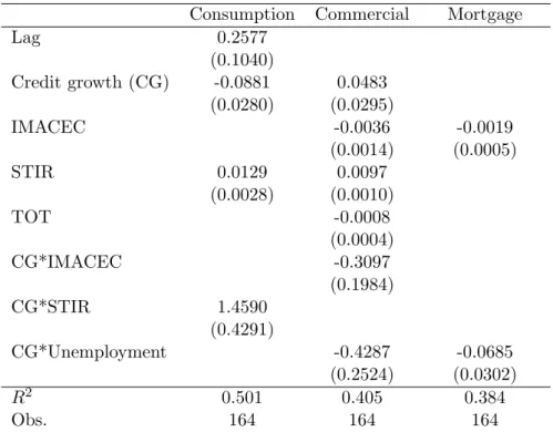
Based on the latest estimation of the model we consider the sample from January 1997 to August 2010. Tables 2 to 4 show the main results for the model. For the case of provisions we can see that the signs of the macroeconomics variables are as expected, and also the overall fit is about 50%. The short-term interest rate has a positive impact meanwhile output growth has a negative one. It is interesting to note that interactions between credit growth and macroeconomics variables are significant as we stated in the theoretical framework. This finding will be relevant for the simulation part as non-linear effects will be generated with this interactions.
The auxiliary equations for write-offs and credit growth show the persistence of those aggre-gates and also the relationship with macroeconomic variables included in the analysis. The fit for consumer credit growth seems reasonable but most of them is due to the seasonal effects and the persistence of the variable. Indeed, removing seasonal dummies the fit is 49% and removing this and the lag structure the fit is only 30%. In the cases of commercial and mortgage credit growth we can see that the fit is relative small (around 20%). This will lead to the fact that in simulations we will have large confidence intervals. Those could overlap under different scenarios. In particular that could imply no difference between baseline and risk scenarios. This problem does not happen in our analysis given that risk scenario is constructed on tail-events and the computed confidence interval do not overlap.
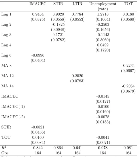
The macroeconomic model is reported in Table 5, there we can see that the sign of the variables are as expected and the overall fit is reasonable for the sample size. It is important to stress that this model is considered only for the dynamic of macroeconomic variables and for that it does not represent the core model used by the bank for conducting Monetary Policy. The latter is based on several dynamics models as VAR and DSGE, and the macroeconomic model presented here is
calibrated to match the dynamic published as baseline scenario in the Monetary Policy Report.
Figure 1: Credit Growth and Loan Loss Provisions Forecasts
Following the steps summarized above in this section we are able to forecast loan loss provisions and credit growth for consumer, commercial and mortgage loans (see Figure 1). Passing those forecasts to the bank level implies to use the current level of loan loss provision and loans as the
initial value of the forecast of each bank. For example a particular bank has total loans forLtwith an initial composition of 70% on consumer, 20% on commercial, and 10% on mortgage. Given that the forecast for Lt+i will be the weighted average of the forecasts for credit growth of each type of loan. In addition to that the cumulated expenditures betweent and t+iare subtracted from earnings which implies that both the Return on Equity (ROE) and the Capital Adequacy Ratio (CAR) moves under the risk scenario. At this point is relevant to note that the model always implies a reduction on ROE but the final effect on CAR depends on the initial position of the bank. Indeed, the data shows that under the Asian crisis in 1998 the CAR for the system exhibited a large increment as result of the strong contraction of credit growth.
Table 2: Results for Provision Model
Consumption Commercial Mortgage
Lag 0.2577 (0.1040) Credit growth (CG) -0.0881 0.0483 (0.0280) (0.0295) IMACEC -0.0036 -0.0019 (0.0014) (0.0005) STIR 0.0129 0.0097 (0.0028) (0.0010) TOT -0.0008 (0.0004) CG*IMACEC -0.3097 (0.1984) CG*STIR 1.4590 (0.4291) CG*Unemployment -0.4287 -0.0685 (0.2524) (0.0302) R2 0.501 0.405 0.384 Obs. 164 164 164
Table 3: Results for Write-Off Model
Consumption Commercial Mortgage
Lag 1 0.4699 0.1808 0.1806 (0.0787) (0.0689) (0.0925) Lag 2 0.2717 (0.0740) IMACEC -0.0114 0.0026 (0.0051) (0.0010) STIR 0.0027 (0.0011) Unemployment 0.0122 0.0012 (0.0017) (0.0002) CG*IMACEC -0.5275 (0.3045) R2 0.353 0.397 0.648 Obs. 164 163 162
Robust standard errors in parentheses. Dummies are not reported.
Table 4: Results for Credit Growth Model Consumption Commercial Mortgage
Lag 1 0.4063 0.1376 (0.0624) (0.1039) Lag 3 0.1276 0.0548 (0.0445) (0.0659) Lag 6 0.3286 (0.0746) IMACEC 0.0885 0.0877 (0.0256) (0.0221) IMACEC(-1) -0.0525 (0.0253) STIR -0.0720 (0.0288) LTIR -0.0794 (0.0322) Write-offs -0.5385 -4.1385 (0.2461) (2.2898) R2 0.604 0.187 0.201 Obs. 164 163 164
Table 5: Results for Macroeconomic Model
IMACEC STIR LTIR Unemployment TOT (rate) Lag 1 0.9454 0.9020 0.7784 1.2718 0.0180 (0.0375) (0.0558) (0.0553) (0.1064) (0.0580) Lag 2 -0.1825 -0.2503 (0.0948) (0.1656) Lag 3 0.1721 -0.1143 (0.0782) (0.3060) Lag 4 0.0492 (0.1720) Lag 6 -0.0996 (0.0404) MA 8 -0.2234 (0.0667) MA 12 0.2020 (0.0783) MA 14 -0.2054 (0.0679) IMACEC -0.0145 (0.0127) IMACEC(-1) -0.0100 (0.0160) IMACEC(-2) -0.0078 (0.0183) STIR -0.0821 (0.0456) TOT 0.0160 -0.0041 (0.0084) (0.0021) R2 0.842 0.864 0.641 0.978 0.081 Obs. 164 164 164 164 164
4
Financial Stability Report
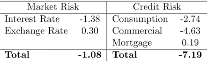
In the previous sections we discussed how the market and credit risks are computed for banks. It should be noted that the latter implies a path of losses which are added on a yearly basis. For that we add the effects up to one year after the shock. The sum of market and credit risks is simple given that both risks are computed in monetary terms: change in the value of the portfolio in the first case and increasing in the loan loss provision in the second. Both can be considered as an increment on expenditures and for that reducing directly the return on equity. Given that the initial value of return on equity is the first buffer to support the increment on expenditures generated by the simulated risk scenario (Table 6).
Table 6: Risk Summary Market Risk Credit Risk Interest Rate -1.38 Consumption -2.74 Exchange Rate 0.30 Commercial -4.63 Mortgage 0.19
Total -1.08 Total -7.19
% of basic capital.
The results obtained are at the bank level and that information is discussed directly with a committee from the SBIF. This is a regular biannual meeting previous to the release of the Financial Stability Report (FSR). The goal of this meeting is to discuss the results obtained in the simulations with the regulator, and for that giving more sense of the numbers. After that qualitative analysis the results are adjusted accordingly and a new set of bank level results are available for the board of the Central Bank. Comments received from the board are discussed again with SBIF team and a final round of results are obtained.
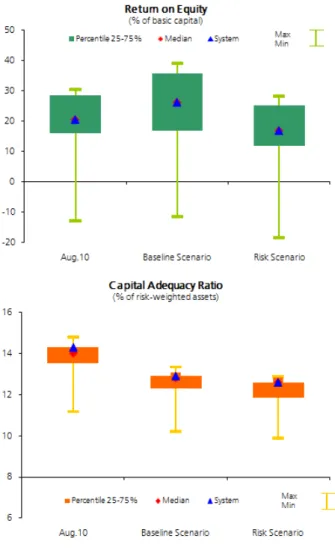
Finally, for the FSR we consider the results for the whole system. Indeed, the details of each risk are summarized at the level of the system and the distribution of banks is presented in a graph where the amount of capital is used as a weight (see Figure 2). In terms of ROE banks exhibiting losses remain in a similar situation under the baseline and risk scenarios, also
over-exposed banks change this indicator dramatically. However, CAR is usually well-above the norm given that most of the bank are well-capitalized. It should be noted that the norm is 8% but in the case of Chile there are financial incentives to be over 10% due to the regulation of the pension funds administrators.
References
Alfaro, R. (2011) “Affine Nelson-Siegel Model,” Economics Letters 110(1): 1-3.
Alfaro, R., D. Calvo, and D. Oda (2009) “Riesgo de Cr´edito de la Banca de Consumo,” Journal
of Chilean Economics12(3): 59-77.
Balduzzi, P., S. Das, and S. Foresi (1998) “The Central Tendency: A Second Factor in Bond Yields,”Review of Economics and Statistics 80: 62-72.
Campbell, J., A. Lo, and A. MacKinlay (1997)The Econometrics of Financial Markets, Prince-ton University Press.
Christensen, J., F. Diebold, and G. Rudebusch (2009) “The Affine Arbitrage-Free Class of Nelson-Siegel Term Structure Models,” Manuscript, University of Pennsylvania.
Cox, J., J. Ingersoll, and S. Ross (1985) “A Theory of the Term Structure of Interest Rates,”
Econometrica53: 385-407.
Diebold, F., and C. Li (2006) “Forecasting the Term Structure of Government Bond Yields,”
Journal of Econometrics130: 337-364.
Hock-Yuen Wong, J., K. Choi, and P. Fong (2008) “A Framework for Stress-Testing Banks’ Credit Risk,” The Journal of Risk Model Validation, 2(1): 3-23.
Hoti, S., E. Maasoumi, M. McAleer, and D. Slottje (2009) “Measuring the Volatility in US Treasury Benchmarks and Debt Instruments,”Econometric Reviews28(5): 522-554. Jara, A., L. Luna, and D. Oda (2007) “Pruebas de Tensi´on de la Banca en Chile,” Financial
Stability Report: Second Half, Central Bank of Chile.
Matus, J. M. (2007) “Indicadores de Riesgo de Cr´edito: Evoluci´on de la Normativa,”Manuscript, Central Bank of Chile.
Nelson, C., and A. Siegel (1987) “Parsimonious Modeling of Yield Curve,”Journal of Business
60(4): 473-489.
Shimer, R. (2008) “The Probability of Finding a Job, ” American Economic Review 98(2): 268-273.
Shreve, S. (2004)Stochastic Calculus for Finance II: Continuous-Time Models, Springer Finance Textbook.
Tapia, C. (2008) “Modelaci´on de Spreads en Mercados Emergentes: Estimaci´on Multi-Familia Usando Filtro de Kalman,”Manuscript, Pontificia Universidad Cat´olica de Chile.
Vasicek, O. (1977) “An Equilibrium Characterization of the Term Structure,”Journal of
Finan-cial Economics 5: 177-188.
Wilmott, P. (2007) Paul Wilmott on Quantitative Finance, Volume 3, Second Edition. John Wiley & Sons, Ltd.
Documentos de Trabajo
Banco Central de Chile
Working Papers
Central Bank of Chile
NÚMEROS ANTERIORES PAST ISSUES
La serie de Documentos de Trabajo en versión PDF puede obtenerse gratis en la dirección electrónica:
www.bcentral.cl/esp/estpub/estudios/dtbc. Existe la posibilidad de solicitar una copia impresa con un costo de $500 si es dentro de Chile y US$12 si es para fuera de Chile. Las solicitudes se pueden hacer por fax: (56-2) 6702231 o a través de correo electrónico: [email protected].
Working Papers in PDF format can be downloaded free of charge from:
www.bcentral.cl/eng/stdpub/studies/workingpaper. Printed versions can be ordered individually for US$12 per copy (for orders inside Chile the charge is Ch$500.) Orders can be placed by fax: (56-2) 6702231 or e-mail: [email protected].
DTBC – 609
Riding the Roller Coaster: Fiscal Policies of Non-renewable Resources Exporters in Latin America and the Caribbean
Febrero 2011
DTBC – 608
Floats, Pegs and the Transmission of Fiscal Policy
Giancarlo Corsetti, Keith Kuester and Gernot J. Müller
Febrero 2011
DTBC – 607
A Bunch of Models, a Bunch of Nulls and Inference About Predictive Ability
Pablo Pincheira
Enero 2011
DTBC – 606
College Risk and Return
Gonzalo Castex
Enero 2011
DTBC – 605
Determinants of Export Diversification Around The World: 1962 – 2000
Manuel R. Agosin, Roberto Álvarez y Claudio Bravo-Ortega
Enero 2011
DTBC – 604
A Solution to Fiscal Procyclicality: the Structural Budget Institutions Pioneered by Chile
Jeffrey Frankel
DTBC – 603
Eficiencia Bancaria en Chile: un Enfoque de Frontera de Beneficios
José Luis Carreño, Gino Loyola y Yolanda Portilla
Diciembre 2010
DTBC – 602
Chile’s Structural Fiscal Surplus Rule: A Model – Based Evaluation
Michael Kumhof y Douglas Laxton
Diciembre 2010
DTBC-601
Price Level Targeting and Inflation Targeting: a Review
Sofía Bauducco y Rodrigo Caputo
Diciembre 2010
DTBC-600
Vulnerability, Crisis and Debt Maturity: Do IMF Interventions Shorten the Length of Borrowing?
Diego Saravia
Noviembre 2010
DTBC-599
Is Previous Export Experience Important for New Exports?
Roberto Álvarez, Hasan Faruq y Ricardo A. López
Noviembre 2010
DTBC-598
Accounting for Changes in College Attendance Profile: A Quantitative Life-cycle Analysis
Gonzalo Castex
Noviembre 2010
DTBC-597
Fluctuaciones del Tipo de Cambio Real y Transabilidad de Bienes en el Comercio Bilateral Chile - Estados Unidos
Andrés Sagner
Octubre 2010
DTBC-596
Distribucion de Probabilidades Implicita en Opciones Financieras
Luis Ceballos
Octubre 2010
DTBC-595
Extracting GDP signals from the monthly indicator of economic activity: Evidence from Chilean real-time data
Michael Pedersen