This is the authors’ accepted manuscript of an article published in the
Journal of Business Finance and Accounting
. The definitive version is
available at www3.interscience.wiley.com.
The Value Premium and Time-Varying Volatility
Xiafei Li*, Chris Brooks** and Joëlle Miffre***
Abstract
Numerous studies have documented the failure of the static and conditional capital asset pricing models to explain the difference in returns between value and growth stocks. This paper examines the post-1963 value premium by employing a model that captures the time-varying total risk of the value-minus-growth portfolios. Our results show that the time-series of value premia is strongly and positively correlated with its volatility. This conclusion is robust to the criterion used to sort stocks into value and growth portfolios and to the country under review (the U.S. and the U.K.). Our paper is consistent with evidence on the possible role of idiosyncratic risk in explaining equity returns, and also with a separate strand of literature concerning the relative lack of reversibility of value firms’ investment decisions.
Keywords: Value premium, Time-varying volatility, CAPM, GJR-GARCH(1,1)-M. JEL classifications: G12, G14.
________________________________
* Nottingham University Business School, Jubilee Campus, Nottingham NG8 1BB, UK,
Xiafei.Li@nottingham.ac.uk
** (Corresponding author) ICMA Centre, University of Reading, Whiteknights, Reading RG6 6BA, U.K., C.Brooks@rdg.ac.uk
*** EDHEC Business School, 393 Promenade des Anglais, BP 3116, 06202 Nice, France,
Joelle.Miffre@edhec.edu
Acknowledgements The authors would like to thank the Editor, Norman Strong, and an anonymous referee for very useful comments on a previous version of this paper. We are also grateful to J. Doukas, H. Lohre, N. Todorovic and seminar participants at the EDHEC-EFM 2008 symposium for their comments. Naturally, all remaining errors are ours.
1.
INTRODUCTION
This paper adds to the asset pricing literature by studying the post-1963 relationship between the value premium and its time-varying volatility, finding that they are positively related. Our measure of time-varying volatility takes into consideration the total and idiosyncratic volatilities of the value and growth portfolios’ returns as described by the family of GARCH (generalised autoregressive conditional heteroskedasticity) models (Engle, 1982; Bollerslev, 1986).1 Within this specification, we also investigate the relationship between the returns of value and growth stocks and their levels of total and idiosyncratic risks.
The rationale for choosing the GARCH(1,1) family of models is twofold. First, our model incorporating a GARCH(1,1) specification explicitly deals with the problem of conditional heteroskedasticity that has plagued studies of the Capital Asset Pricing Model (CAPM). As well as having constant betas, the static CAPM also assumes that the variances of the error terms are constant. However, numerous researchers have found that for financial time series, the variances of the error terms change over time in a partially predictable fashion (see, for example, French et al., 1987; Schwert and Seguin, 1990) and exhibit volatility clustering, where large (small) volatility changes tend to be followed by large (small) volatility changes. Our model suitably relaxes the assumption of homoscedasticity in the disturbances by capturing the impact of new information (as measured by the error term) on the conditional variance of the portfolio’s returns through the most recent squared error. Second, our model explicitly includes the conditional volatility of portfolio returns (as modelled by the GARCH(1,1)-in-mean of Engle et al., 1987) in the mean equation. The essence of the argument for doing so is that the release of new information (captured by the error term) may cause the risk (conditional variance) of the value and growth portfolios to change over time in a way that is priced and can be captured by our model.
While the outperformance of value stocks relative to growth stocks is commonly accepted, interpreting the premium and identifying its causes has been more controversial. Two explanations have been put forward. The behavioural explanation, presented by Lakonishok et
1
Within this class of models, we follow the vast majority of studies in this area in using the most parsimonious specification, the GARCH(1,1) form.
al. (1994), La Porta (1996) and La Porta et al. (1997), attributes the value premium to investors’ judgment biases and to the systematic forecast errors that they make while extrapolating past performance.2 The second explanation argues that markets are efficient and that the value premium is compensation for risk. Both static and conditional versions of the CAPM and the Consumption CAPM have been used to study the outperformance of value stocks. Unfortunately the results are mixed3 and thus the question remains as to whether the value premium conforms to an asset pricing model.
We make two contributions to the asset pricing literature that are worth noting. First, we find a positive relation between the value premium and its conditional volatility. We also show that value stocks have greater exposure to their conditional volatility than growth stocks and thus earn a higher return.4 Second, these conclusions are robust to the criterion used to sort stocks into value or growth portfolios (B/M, C/P and E/P) and to the country under review (the U.S. versus the U.K.).
We offer two possible explanations for our finding of a positive relation between the value premium and its conditional volatility. The first relates to the static CAPM missing a systematic risk factor that correlates with the conditional volatility of the value premium and possibly with the business cycle (Kogan, 2004; Zhang, 2005). The argument, which we detail in Section 2.2,
2 As a result, investors underprice out-of-favour (value) stocks and overprice glamour (growth) stocks.
Eventually, overly enthusiastic growth investors are disappointed by the poor earnings announcements of growth stocks while overly pessimistic value investors are pleasantly surprised. The market then corrects previous mis-pricings such that value stocks become winners and growth stocks become losers. However, Michou (2009) shows that, in a time-series context, the value spread is a poor predictor of the returns on various stock portfolios.
3 Fama and French (2006) and Ang and Chen (2007) find that the static CAPM captures the value premium
of 1926-1963, but fails to explain it for the post-1963 period. Conditional versions of both the CAPM and the consumption CAPM have been shown to perform substantially better than their static counterparts (Jagannathan and Wang, 1996; Lettau and Ludvigson, 2001). Yet the ability of the conditional CAPM to capture the value premium is still open to debate. Using a conditional consumption CAPM, Lettau and Ludvigson (2001) show that the value premium is attributable to the high conditional risk of value stocks, a result echoed by Adrian and Franzoni (2005) and Ang and Chen (2007). Along the same lines, Petkova and Zhang (2005) find that the conditional betas of the value-minus-growth strategies are higher in bad states of the economy. However, the conclusions of these papers are put into question by Fama and French (2006) and Lewellen and Nagel (2006), who argue that variations in market betas are not large enough to fully explain the outperformance of value stocks.
4
This work is, in spirit, related to that presented in Li et al. (2008), who show that momentum profits are related to time-varying risk.
relates to the counter-cyclical nature of the value premium and its conditional volatility. Since our measure of total risk uses a GARCH(1,1) specification and thus depends on both past return volatility and past idiosyncratic risk, a second explanation lends support to the idea that the value premium may relate to a lack of diversification of the value and growth portfolios. This result is in line with the notion that agents who fail to fully diversify their portfolios demand higher average returns to compensate them for holding larger levels of firm-specific risk (Merton, 1987).
The remainder of the paper is organised as follows. Section 2 develops a model for time-varying risk within a GARCH(1,1)-M framework and discusses the econometric specifications. Section 3 describes the data. Sections 4 and 5 report the empirical results for U.S. and U.K. data, respectively. Section 6 provides an analysis of the findings and finally, Section 7 offers some concluding remarks.
2.
ECONOMETRIC FRAMEWORK
1. The Static CAPM
Letting rit and rMt denote excess returns on asset i and on the market portfolio of all assets in period t, the static CAPM of Sharpe (1964) can be written as follows
rit iE
rMtE
where
i Cov
rit,rMt
/Var
rMt , and E
. , Cov
. and Var
. denote expectation, covariance and variance, respectively. This static CAPM assumes that the ratio of the expected asset excess return to the expected market excess return remains constant over time, that is, all investors have the same expectations about asset returns for any given time period. However, in practice investors may update their expectations each period according to new information and this leads to conditional expectations, which are stochastic rather than constant.2. Model Specifications
We start by considering the static CAPM in ex-post form given by model (1)
Mt ft
PtPt R R
r
(1)high-minus-low (HML) portfolio of Fama and French (1993), RMt is the value-weighted return on the market portfolio of all assets, Rft is the one-month Treasury bill rate and
0, 2~
Pt N . If the static CAPM is valid, alpha should equal zero.
The market model with a standard GARCH(1,1) process (Bollerslev, 1986) for the conditional variance of portfolio returns is given by model (2)
1 2 1 Pt Pt Pt Pt ft Mt Pt h h R R r
(2)where Pt ~ N
0,hPt
, hPt is the conditional variance of portfolio returns, and , , and are parameters to estimate. To ensure that hPt is non-negative, non-degenerate and that the GARCH(1,1) process is covariance stationary, the conditions
0,0
1, 0
1 and 1 are imposed. The market model with a GARCH specification for the conditional variance allows expected excess returns, and the conditional variances and covariances of asset returns to vary over time. The conditional variance depends on both the square of past return shocks (past idiosyncratic risk) and past realisations of the conditional variance itself (past total risk).According to Nelson (1991), Glosten et al. (1993) (hereafter GJR) and Rabemananjara and Zakoian (1993), good news (measured by positive return shocks) and bad news (measured by negative return shocks) may have an asymmetric impact on the conditional variance of stock returns. In particular, it has been shown that volatility is higher for negative returns than positive returns of the same magnitude. This has been argued to arise either from “leverage” (the impact of falling versus rising stock prices on a firm’s debt-to-equity ratio) or “volatility feedback” effects. In model (3), we explicitly capture this potential asymmetric effect and test whether value and growth stocks respond in the same way to good and bad news. Therefore we obtain
1 2 1 1 2 1 Pt Pt t Pt Pt Pt ft Mt Pt h I h R R r
(3)where measures any asymmetric response of volatility to good and bad news,
Pt
Pt ~ N 0,h
conditions for non-negative and non-degenerate hPt and covariance stationarity are 0
,0 1, 0 1,
0 and
/2
1.In models (4) and (5), we follow Engle et al. (1987) and add to (2) and (3) a conditional standard deviation term in the mean equation that captures the time-varying risk premium of value and growth stocks. The resulting models are as follows
1 2 1 Pt Pt Pt Pt Pt ft Mt Pt h h h R R r (4)
1 2 1 1 2 1 Pt Pt t Pt Pt Pt Pt ft Mt Pt h I h h R R r (5) where Pt ~ N
0,hPt
and measures the loading of the portfolio return on its time-varying conditional volatility hPt . These models imply that increased risk as measured by the conditional standard deviation leads to a rise ( > 0) or fall ( < 0) in the level of compensation for holding the asset.Following Nelson (1991) and Hentschel (1995), for the sake of comparison and completeness, we adopt another commonly used functional form for capturing the time-varying risk in models (6) and (7), which instead of the conditional standard deviation, uses the conditional variance in the mean equation. Therefore, we obtain
1 2 1 Pt Pt Pt Pt Pt ft Mt Pt h h h R R r
(6)
1 2 1 1 2 1 Pt Pt t Pt Pt Pt Pt ft Mt Pt h I h h R R r (7)where Pt ~ N
0,hPt
and measures the loading of the portfolio return on its time-varying conditional variance hPt. Models (4) to (7) imply that there are serial correlations in asset returns arising through the introduction of the conditional variance, which is itself autocorrelated, in the mean equation. In addition, the conditional expected portfolio return is a linear function of the conditional variance.investment of Kogan (2004) and Zhang (2005), where capital purchases are either irreversible or costly to reverse. Kogan (2004) uses a general equilibrium model to examine the relationship between asset prices and real investment. He shows that the conditional volatility of stock return is related to the real economy, and rigidities in the investment process give relevance within the model to the book-to-market ratio because it proxies for states of the economy. When the ratio takes relatively low values, its relationship with volatility is negative, but it is positive when the ratio is high because the irreversibility of investment decisions makes the conditional volatility of value firms more countercyclical than that of growth firms.
The key insight in Zhang’s (2005) study is to consider the value anomaly at the level of the firm’s production. The intuition is that the risk premium is counter-cyclical, that is, it is higher when the economy is in recession, and also that reversing existing investments in capital is costly. Therefore, in bad states of the economy, value firms will be burdened by more capital than they need but face large costs if they wish to reduce capacity. Growth firms, on the other hand, hold options to expand but will not have such excess capacity when demand falls. The time-varying nature of the risk premium implies that the relatively high cost of this capital for value firms will be most severe exactly when it is least productive, which results in the value premium being counter-cyclical.
If the theoretical predictions from the models of Kogan (2004) and Zhang (2005) are brought together, we conjecture that the value premium and its conditional volatility are positively correlated over time because they are both counter-cyclical. In order to test this conjecture, we examine in models (4) to (7) the null hypothesis that the value premium is compensation for time-varying risk, which implies that either or (depending on the model) is statistically significant and positive. We also analyze the impact on the volatility of the value and growth portfolio returns of more recent information (as measured by ), of older information (as measured by ) and of negative versus positive return shocks (as measured by in models (3), (5) and (7)).
3.
DATA
Our U.S. data comprise portfolios that include all NYSE, AMEX, and NASDAQ stocks.5 At the end of June, all stocks are ranked into decile portfolios based on the ratios of B/M, C/P or E/P. The stocks in the portfolios are value-weighted and the positions are held over the following 12 months, when the portfolios are re-formed. A value portfolio contains the top 10% of stocks ranked by each ratio and a growth portfolio contains stocks in the bottom 10%. HML is the return of a more or less size-neutral portfolio that is long value and short growth (Fama and French, 1993). The sample covers the period July 1963 to June 2006. The value-weighted return on all NYSE, AMEX, and NASDAQ stocks in excess of the one-month Treasury bill rate is used as a proxy for the market risk premium.
In order to provide comparative evidence for a different market, we first examine the U.K. return series of value and growth portfolios sorted on B/M, C/P and E/P from K. French’s website. At the end of December each year, all stocks listed on the U.K. stock market are ranked into 3 groups based on their B/M, C/P or E/P ratio. This time, the value portfolio contains stocks in the top 30% and the growth portfolio contains stocks in the bottom 30%. The value premium in French’s U.K. dataset is only significant and positive when the portfolio construction is based on C/P and E/P. Possibly due to the different ranking method and sample period from the U.S., the high B/M U.K. portfolio does not significantly outperform the low B/M U.K. portfolio over the 1975 to 2001 period.6 By contrast, Dimson et al. (2003) report a strong value premium (when value is measured by B/M) in the U.K. stock market over the period 1955 to 2001. Unlike French who uses for the U.K. the 30%, 40% and 30% breakpoints, the value (growth) portfolio of Dimson et al. (2003) contains stocks in the top (bottom) 40% by B/M ranking. Therefore, in order to investigate the value premium, in all subsequent tests using U.K. data in this study, we use the B/M series of Dimson et al. (2003)7 and the C/P and E/P series of K. French. The sample period runs from January 1963 to December 2001 for the B/M portfolios and from January 1975 to December 2001 for the C/P and E/P portfolios.
5 The return series of portfolios are downloaded from K. R. French’s website. 6
Fama and French (1998) report a similar result for the period 1975 to 1995.
4.
THE U.S. VALUE PREMIUM
This section analyzes the mean returns of the U.S. B/M, C/P and E/P portfolios and their performance within the static CAPM (subsection 1). We then explicitly test whether the post-1963 returns of the value, growth and HML portfolios relate to their time-varying risk, as described by different specifications of the GARCH(1,1) model (subsection 2).
1. Summary Statistics of the Value Premium and Performance within the Static CAPM
Panel A of Table 1 presents summary statistics for the monthly returns of the U.S. B/M, C/P and E/P portfolios. High represents a value portfolio containing stocks in the top 10% of each ratio, while Low represents a growth portfolio containing stocks in the bottom 10% of each ratio. HML measures the value premium as the return of a long value, short growth portfolio. The t-statistics reported in Table 1 are for the significance of the mean based on heteroskedasticity- and autocorrelation-robust (Newey and West, 1987) standard errors.
<< Insert Table 1 around here >>
Consistent with the evidence in Fama and French (1992, 1993, 2006), Davis et al. (2000) and Ang and Chen (2007), we find that the B/M-sorted growth portfolio has a low mean return of 0.81%. By contrast, the value portfolio has high mean returns of 1.39% per month. As a result, there is a reliable value premium in returns. The value premium is 0.57% per month on average and is significant at the 1% level (t = 2.88). The monthly mean returns of the C/P and E/P-sorted portfolios are of a similar magnitude to those of the B/M portfolios.
Panel B of Table 1 reports OLS estimates of the static CAPM for the B/M, C/P and E/P portfolios. The results confirm the findings of Fama and French (1992, 1993, 2006) and Ang and Chen (2007) that for the post-1963 period, the static CAPM is rejected for the B/M, C/P and E/P value premia since the α coefficients of 0.62%, 0.59% and 0.69% per month respectively are significant at the 1% level. The goodness of fit statistics confirm this finding since the R2 values are a mere 1% to 5%. It is also evident that the value portfolios have less market risk (lower betas) than the growth portfolios. The market betas of the C/P and E/P HML portfolios are negative and significant at the 1% level, while the market beta of the B/M HML portfolio is negative though insignificant (β = -0.11, t = -1.69).
If the static CAPM is an adequate characterisation of the temporal variation in returns, the variances of the error terms should be constant. This motivates us to perform a series of Lagrange Multiplier (LM) tests to assess the validity of the static CAPM under the null hypothesis that there is no autoregressive conditional heteroskedasticity (ARCH) (Engle, 1982) in the errors. Following previous studies in the time-series literature, we test for ARCH-effects of order up to 5. The test statistic is asymptotically distributed as a 2 with 5 degrees of freedom under the null hypothesis of no ARCH. The results, reported in Panel B of Table 1, clearly indicate that the B/M, C/P and E/P value, growth and HML portfolios period show substantial evidence of ARCH effects as the LM statistics are significant at the 5% level or better. Therefore, it is perhaps no surprise to see that the static CAPM cannot explain the post-1963 value premium.
2. The Value Premium within a GARCH Framework
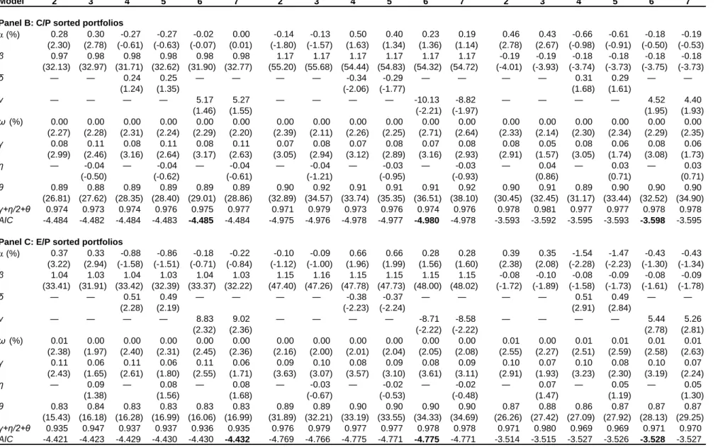
In order to allow for heteroskedasticity (and autocorrelation) in the errors of the CAPM for the value, growth and HML portfolios, we assume that the conditional variances of portfolio returns follow a GARCH(1,1) process. Table 2 presents the estimates of models (2) to (7) for the value, growth and HML portfolios. The decision to allocate a stock to either the value or growth portfolio is based on B/M in Panel A, on C/P in Panel B and on E/P in Panel C. The estimation method is Maximum Likelihood with Bollerslev-Wooldridge robust standard errors. Akaike information criterion (AIC) values are also reported in Table 2.8
<< Insert Table 2 around here >>
Portfolios Sorted on B/M
Table 2, Panel A reports estimates of the model that includes GARCH(1,1) and GJR-GARCH(1,1) specifications for the errors (models (2) and (3)). In model (2), the market beta of the value portfolio is 0.96 (t = 28.04) and that of the growth portfolio is 1.09 (t = 48.91). Although the value premium seems prima facie to have less market risk than the growth portfolio, the beta of the HML portfolio is insignificant, albeit negative (β = -0.07, t = -1.5),
8 AIC is a function of the maximised value of the log-likelihood function and is used to compare the relative
merits of models; a model with the lowest value of AIC is preferred. The rationale for reporting AIC instead of R2 is that the former is designed for any model while the latter is only applicable for linear regression models and will not reflect any goodness of fit in the conditional variance equation.
implying that the CAPM cannot explain the positive B/M value premium. The coefficient measures the impact of recent information on volatility and is equal to 0.13 for the value portfolio and 0.04 for the growth portfolio, indicating that recent information has a stronger impact on the volatility of value stocks than on that of growth stocks. The coefficient captures the impact of historical information on volatility and is equal to 0.85 for the value portfolio and 0.94 for the growth portfolio, suggesting that older information has less influence on the volatility of the value portfolio than on that of the growth portfolio. The positive and significant
and coefficients also suggest that both historical and more recent information have strong impacts on the volatility of the value, growth and HML portfolios.
Model (3) allows good news and bad news to have an asymmetric impact on volatility of portfolio returns by adding a leverage effect term,
It1
Pt21, to the variance equation of model(2). The estimated value of this parameter for the value portfolio is 0.07, which is statistically insignificant (t = 1.01). Thus, no matter whether the announcement represents good or bad news, the impact on the volatility of the value portfolio is symmetric. The same conclusion applies to the HML portfolio. On the other hand, for the growth portfolio is -0.05, which is statistically significant at the 5% level. Therefore, after an announcement of good news, the volatility of the growth portfolio increases more than after the announcement of bad news.
Models (4) and (5) add a time-varying risk premium,
hPt , to the mean equations of models (2) and (3). The results show that the excess return of the value portfolio is positively related to its time-varying risk as the δ coefficient of model (4) is 0.35 (t = 2.16) and that of model (5) is 0.33 (t = 2.07). Conversely, the excess return on the growth portfolio is negatively related to its time-varying risk as the δ coefficient of model (4) is -0.32 (t = -2.04) and that of model (5) is -0.23 (t = -1.69). Therefore, the value portfolio appears to be more sensitive to its conditional time-varying risk than the growth portfolio (Value > Growth). As a result, the expected return of the HML portfolio is positively and significantly related to its time-varying risk as the δ coefficient of (4) is 0.50 (t = 2.46) and that of (5) is 0.46 (t = 2.36).Models (6) and (7) use the conditional variance to replace the conditional standard deviation as a time-varying measure of risk in the mean equations of models (4) and (5). Most of the
estimates from these two models are similar to those of models (4) and (5). The loading on time-varying risk, ν, of the HML portfolio is 5.63 (t = 2.48) for model (6) and 5.28 (t = 2.46) for model (7). Both are statistically significant at the 5% level. The AIC figures are lowest for models (6) and (7), which support the finding that these models are better suited to model the value premium.
Portfolios Sorted on C/P and E/P
Panels B and C present similar results to Panel A, but this time we use C/P and E/P as the criteria on which to sort stocks into value or growth portfolios. The value portfolio has less market risk than the growth portfolio since the average market beta is 0.98 (1.03) for the C/P (E/P) value portfolio and 1.17 (1.15) for the C/P (E/P) growth portfolio. Since the market beta of the HML portfolio is negative and significant at the 1% or 10% level, it fails to explain the post-1963 positive C/P and E/P value premium. As for the B/M sort, the loadings on conditional risk, δ and ν, are positive for the value portfolios and negative for the growth portfolios. This suggests that the value portfolios are more sensitive to their time-varying total risk than the growth portfolios. Time-varying total risk plays a central role in explaining the C/P and E/P value premium too as the loadings on time-varying risk of model (6) (ν = 4.52 in Panel B and ν = 5.44 in Panel C) and model (7) (ν = 4.4 in Panel B and ν = 5.26 in Panel C) are statistically significant at either the 1% or 10% level. The AIC values for the HML portfolios in Panels B and C also suggest that system (6) best models the premium.9
Overall, the results of the C/P and E/P portfolios are consistent with our findings for the B/M portfolios: the value premium directly relates to the conditional volatility of the value and growth portfolios, with the value (growth) portfolio having a positive (negative) loading on conditional volatility. This intuitively suggests that the dispersion in returns between value and growth relates to their different responses to a change in time-varying total risk.10
9 In addition, we carry out a series of ARCH LM test for the residuals of models (2) to (7) for the value,
growth and HML portfolios and find that the test statistics are statistically insignificant, suggesting that there is no evidence of ARCH effects in the errors after using our GARCH(1,1) specifications.
10 Loughran (1997), Daniel and Titman (1997), Davis et al. (2000) and Fama and French (2006) report that
the post-1963 value premium is greater for small capitalisation stocks than for large capitalisation stocks. Their results raise a question as to whether the size effect can explain the post-1963 value premium. We examine this hypothesis by adding a Fama and French (1993)-style size factor to models (2) to (7) described
5.
THE U.K. VALUE PREMIUM
Using U.S. data, we show above that the conditional model incorporating a GARCH(1,1)-M specification best models the post-1963 value premium. However, in order to ensure that these results are not an artifact unique to this market, we conduct in this section a comparison in which we reapply the models to the U.K. market.
Table 3 reports summary statistics for monthly returns on the U.K. value, growth and HML portfolios (Panel A) and tests the ability of the standard CAPM to explain the value premium (Panel B). Consistent with the U.S. evidence, the value premia in returns are 0.5%, 0.42% and 0.36% per month for the B/M, C/P and E/P HML portfolios, respectively. They are statistically significant at the 10% level or better. The unconditional standard deviation of the B/M-sorted value portfolio (at 5.22%) is similar to that of the B/M-sorted growth portfolio (at 5.26% per month). Thus, the results of Table 3 confirm the U.K. findings of Gregory et al. (2001, 2003) that the value premium is not a compensation for total unconditional risk.
<< Insert Table 3 around here >>
The alphas for the B/M, C/P and E/P HML portfolios in Table 3, Panel B are 0.52%, 0.77% and 0.60% per month, respectively; all of these are significant at the 5% level or better. The CAPM betas of the HML portfolios are statistically insignificant. These results provide comparative evidence that the static CAPM is rejected for the U.K. value premium. In order to examine the statistical validity of the static CAPM for U.K. data, Table 3, Panel B reports the ARCH-LM statistics and associated p-values. The results show that the LM statistics are significant at the 5% level or better in all cases: all the U.K. value, growth and HML portfolios, irrespective of the sorting criteria used, have ARCH effects in their errors. This indicates that the models are mis-specified, and so it is perhaps not surprising that the static CAPM fails to explain the U.K. value premium.
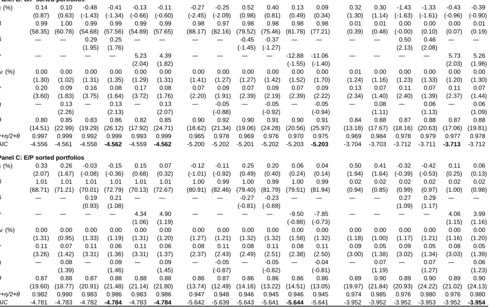
Table 4 presents the parameter estimates of models (2) to (7) for the U.K. value, growth and HML portfolios. Overall, the U.K. results fully support the conclusions from the U.S. data. First,
above. The evidence from Table 2 is robust to the inclusion of a size factor in the mean equation of the market model with a GARCH specification and hence these results are not presented to conserve space.
while the market betas of the value and growth portfolios are positive and significant at the 1% level, the betas of the HML portfolios are statistically insignificant at the 5% level, confirming that the static model cannot explain the value premium. Second, the loadings on conditional risk, δ and ν, of models (4) to (7) are positive for the value portfolios and negative for the growth portfolios, suggesting that the performance of the value and growth portfolios critically relates to their time-varying total risk. Third, the value premia are positively related to the conditional volatilities of the HML portfolios.
<< Insert Table 4 around here >>
6.
INTERPRETATION OF THE RESULTS
How can the result that time-varying measures of total risk are correlated with the value premium be rationalised? One possible explanation is that the conditional volatility GARCH(1,1)-M term is related to a risk factor that is missing from existing asset pricing specifications. But what might be the nature of this risk factor? We offer three potential explanations.
Doukas et al. (2004) provide a possible answer by relating the outperformance of value stocks to the greater disagreement characterising their future growth in earnings. They show that because beliefs regarding the future prices of value stocks are more heterogeneous than for growth stocks, value stocks are perceived as more risky and thus earn more, a finding consistent with our results.
Another possible justification based on the business cycle could be brought forward as an explanation for the higher loadings on conditional volatility (as measured by and ), and thus the better performance of value stocks. The time-varying risk premium
hPt in (4) and (5) and hPt in (6) and (7) that we identify for value stocks possibly relates to the higher costs of value firms in reversing existing investment in capital in periods of recession as discussed in Section 2 above (see Kogan, 2004; or Zhang, 2005).11 The implication is then that value firms
11
In bad states of the economy, value firms are burdened by more capital than they need and face large costs if they wish to reduce capacity. The relatively high cost of this capital for value firms will be most severe
are indeed more risky than growth firms when risk is thought of as the possibility that the firm will be stuck with excess capacity that it cannot use or sell off in adverse states of the world. Along the same lines, Fama and French (1996) conjecture that the value premium is priced as a risk factor because it is related to investment opportunities, a suggestion that is given credence empirically by Hahn and Lee (2006) and Petkova (2006) using financial variables that can capture such opportunities. It is worth noting however that Gregory et al. (2003) find no evidence that value stocks perform poorly in poor market conditions, in effect ruling out the business cycle explanation for the U.K.
Since our measure of total risk uses a GARCH(1,1) specification and thus depends on both past return volatility and past idiosyncratic risk, a third explanation to account for the observed positive relation between the value premium and time-varying volatility relates to the idea that idiosyncratic risk commands a risk premium (Merton, 1987). While the value and growth portfolios comprise sufficiently large numbers of stocks that most academics and market practitioners would consider them well diversified, the compositions are not proportionately stratified from an industrial perspective. It is widely known that value portfolios tend to attach disproportionately large weights to utilities, mining, and basic manufacturing companies whereas growth portfolios imply disproportionately large bets on technology, software, advertising and pharmaceutical companies, for example. This lack of diversification could lead to persistent non-trivial level of unsystematic risk in the two portfolios. Supporting evidence for this hypothesis is provided in Campbell et al. (2001) who argue that 50 randomly selected stocks are now needed to achieve full diversification. In our case, stocks in the value and growth portfolios are not randomly selected but are drawn from similar industries. Thus, despite their large number of stocks, the value and growth portfolios might fail to reach complete diversification. It is possible that the remaining idiosyncratic risk commands a risk premium that is unrelated to the CAPM beta and is captured by our conditional GARCH model. Our paper therefore could indirectly contribute to the debate on the possible role of unsystematic risk in explaining stock returns 12
exactly when it is least productive; namely, in periods of recessions. Growth firms, on the other hand, hold options to expand, thus they do not have such excess capacity when demand falls.
7.
CONCLUSIONS
The puzzle that the static CAPM fails to capture the post-1963 value premium, variously defined, has been a concern in the financial literature for over a decade. This paper adds to the static CAPM a conditional volatility term and tests whether this conditional specification is related to the value premium and to the performance of value and growth stocks. We draw two main conclusions from our analysis. First, the time series of value premia is strongly and positively related with conditional volatility as modelled by GARCH(1,1)-M terms. Second, this finding is robust to the sorting technique used to define value and growth and to the choice of the stock market under investigation (U.S. versus U.K.).
Our primary finding that the value premium is highly positively correlated with its time-varying volatility is consistent with the notion, put forward by Fama and French (1996), Kogan (2004), Zhang (2005), Hahn and Lee (2006) and Petkova (2006), that HML may proxy the business cycle. Hence it may be that the CAPM in its static form is mis-specified: it omits a risk factor that is proxied by the conditional volatility of the portfolio returns. This risk factor relates to differences in the amount of investment capital that value and growth firms possess and the difficulties that value firms have in reducing such investments during economic downturns.
An alternative explanation is that the positive correlation between time-varying total risk and the value premium may arise from the ability of conditional volatility to capture the unsystematic risk present in the value and growth portfolios. Our result could instead give credence to recent empirical findings that relate stock returns to a lack of diversification and idiosyncratic risk (Merton, 1987; Goyal and Santa-Clara, 2003; Ghysels et al., 2005; Jiang and Lee, 2006; Diavatopoulos et al., 2008; Fu, 2009). Since the relation between average return and idiosyncratic risk has been found to be positive (Goyal and Santa-Clara, 2003; Ghysels
et al., 2005; Fu, 2009; Jiang and Lee, 2006; Diavatopoulos et al., 2008) as well as negative average returns, Goyal and Santa-Clara (2003), Ghysels et al. (2005), Fu (2009), Jiang and Lee (2006) and Diavatopoulos et al. (2008) find the opposite, namely a positive relation between idiosyncratic risk and stock market returns. Bali et al. (2005) and Bali and Cakici (2008) argue that the results of Goyal and Santa-Clara (2003) could be spuriously driven by small illiquid stocks traded on the Nasdaq and critically depend on the measure of idiosyncratic volatility used, the sample studied and data frequency.
(Ang et al., 2006, 2009), we are tempted to conjecture that the argument based on the irreversibility of investments is the most compelling explanation for our results. However, we have not tested this hypothesis empirically and we see disentangling the two explanations as an interesting topic for future research. Should neither hypothesis be supported by the data, then one would be forced to conclude as in Gregory et al. (2003) that the return of value investment strategies relates to a mispricing story à la Lakonishok et al.
REFERENCES
Adrian, T., F. Franzoni (2005), ‘Learning about Beta: Time-Varying Factor Loadings, Expected Returns, and the Conditional CAPM’, Working Paper (Federal Reserve Bank of New York and HEC School of Management, Paris).
Ang, A., J. Chen (2007), ‘The CAPM over the Long-Run: 1926-2001’, Journal of Empirical Finance, Vol. 14, pp. 1–40.
Ang, A., R. J. Hodrick, Y. Xing, X. Zhang (2006), ‘The Cross-Section of Volatility and Expected Returns’, Journal of Finance, Vol. 61, pp. 259-299.
Ang, A., R. J. Hodrick, Y. Xing, X. Zhang (2009), ‘High Idiosyncratic Volatility and Low Returns: International and Further U.S. Evidence’, Journal of Financial Economics
Vol. 19, pp. 1-23.
Bali, T. G., and N. Cakici (2008), ‘Idiosyncratic Volatility and the Cross-Section of Expected Returns’, Journal of Financial and Quantitative Analysis, Vol. 43, pp. 29-58.
Bali, T. G., N. Cakici, X. Yan, Z. Zhang (2005), ‘Does Idiosyncratic Risk Really Matter?’,
Journal of Finance, Vol. 60, pp. 905-929.
Bollerslev, T. (1986), ‘Generalized Autoregressive Conditional Heteroskedasticity’, Journal of Econometrics, Vol. 31, pp. 307-327.
Campbell, J. Y., M. Lettau, B. G. Malkiel, Y. Xu (2001), ‘Have Individual Stocks Become more Volatile? An Empirical Exploration of Idiosyncratic Risk’, Journal of Finance, Vol. 56, pp. 1-43.
Daniel, K., S. Titman (1997), ‘Evidence on the Characteristics of Cross Sectional Variation in Stock Returns’, Journal of Finance, Vol. 52, pp. 1-33.
Davis, J., E. F. Fama, K. R. French (2000), ‘Characteristics, Covariances, and Average Returns: 1927-1997’, Journal of Finance, Vol. 55, pp. 389-406.
Diavatopoulos, D., J. S. Doran, D. R. Peterson (2008), “The Information Content in Implied Idiosyncratic Volatility and the Cross-Section of Stock Returns: Evidence from the Option Markets”. Journal of Futures Markets, Vol.28, pp. 1013-1039.
Dimson, E., S. Nagel, G. Quigley (2003), ‘Capturing the Value Premium in the United Kingdom’, Financial Analysts Journal, Vol. 59, pp. 35-45.
Doukas, J. A., C. F. Kim, C. Pantzalis (2004), ‘Divergence of Opinions and the Performance of Value Stocks’, Financial Analysts Journal, Vol. 60, pp. 55-64.
Engle, R. F. (1982), ‘Autoregressive Conditional Heteroskedasticity with Estimates of the Variance of United Kingdom Inflation’, Econometrica, Vol. 50, pp. 987-1008.
Engle, R.F., D.M. Lilien and R.P. Robins (1987), ‘Estimating Time-varying Risk Premia in the Term Structure: The ARCH-M Model, Econometrica, Vol. 55, pp. 391-407. Fama, E. F., K. R. French (1992), ‘The Cross-Section of Expected Stock Returns’, Journal of
Fama, E. F., K. R. French (1993), ‘Common Risk Factors in the Returns on Stocks and Bonds’, Journal of Financial Economics, Vol. 33, pp. 3-56.
Fama, E. F., K. R. French (1996), ‘Multifactor Explanations of Asset Pricing Anomalies’,
Journal of Finance, Vol. 51, pp. 55-84.
Fama, E. F., K. R. French (1998), ‘Value versus Growth: The International Evidence’,
Journal of Finance, Vol. 53, pp. 1975-1999.
Fama, E. F., K. R. French (2006), ‘The Value Premium and the CAPM’, Journal of Finance, Vol. 61, pp. 2163-2185
French, K. R., G. W. Schwert, R. F. Stambaugh (1987), ‘Expected Stock Returns and Volatility’, Journal of Financial Economics, Vol. 19, pp. 3-30.
Fu, F. (2009), ‘Idiosyncratic Risk and the Cross-Section of Expected Stock Returns’, Journal of Financial Economics Vol. 91, pp. 24-37.
Ghysels E., P. Santa-Clara and R. I. Valkanov (2005), ‘There is a Risk-Return Tradeoff after All’, Journal of Financial Economics, Vol. 76, pp. 509-548.
Glosten, L. R., R. Jagannathan, D. E. Runkle (1993), ‘On the Relation between the Expected Value and the Volatility of the Nominal Excess Return on Stocks’, Journal of Finance,
Vol. 48, pp. 1779-1801.
Goyal, A., P. Santa-Clara (2003), ‘Idiosyncratic Risk Matters!’, Journal of Finance, Vol. 58, pp. 975-1007.
Gregory, A.; R. Harris, and M. Michou (2001), ‘An Analysis of Contrarian Investment Strategies in the UK’, Journal of Business Finance and Accounting, Vol. 28, pp. 1931-1228.
Gregory, A.; R. Harris, and M. Michou (2003), ‘Contrarian Investment and Macroeconomic Risk’, Journal of Business Finance and Accounting, Vol. 30, pp. 213-254.
Hahn, J., H. Lee (2006), ‘Yield Spreads as Alternative Risk Factors for Size and Book-to-Market’, Journal of Financial and Quantitative Analysis, Vol. 41, pp. 245-269.
Hentschel, L. (1995), ‘All in the Family Nesting Symmetric and Asymmetric GARCH Models’, Journal of Financial Economics, Vol. 39, pp. 71-104.
Jagannathan, R., Z. Wang (1996), ‘The Conditional CAPM and the Cross-Section of Expected Returns’, Journal of Finance, Vol. 51, pp. 3-53.
Jiang X. and B.-S. Lee (2006), ‘The Dynamic Relation between Returns and Idiosyncratic Volatility’, Financial Management Vol. 35, pp. 43-65.
Kogan, L. (2004), ‘Asset Prices and Real Investment’, Journal of Financial Economics, Vol. 73, pp. 411-431.
Lakonishok, J., A. Shleifer, R. Vishny (1994), ‘Contrarian Investment, Extrapolation, and Risk’, Journal of Finance, Vol. 49, pp. 1541-1578.
LaPorta, R. (1996), ‘Expectations and the Cross Section of Stock Returns’, Journal of Finance, Vol. 51, pp. 1715-1742.
LaPorta, R., J. Lakonishok, A. Shleifer and R. Vishny (1997), ‘Good News for Value Stocks: Further Evidence on Market Efficiency’, Journal of Finance, Vol. 52, pp. 859-874. Lettau, M., S. Ludvigson (2001), ‘Resurrecting the (C)CAPM: A Cross-Sectional Test when
Risk Premia are Time-Varying’, Journal of Political Economy, Vol. 109, pp. 1238-1287.
Lewellen, J., S. Nagel (2006), ‘The conditional CAPM does not Explain Asset-Pricing Anomalies’, Journal of Financial Economics, Vol. 82, pp. 289-314.
Li, X., J. Miffre, C. Brooks, N. O’Sullivan (2008), ‘Momentum Profits and Time-Varying Unsystematic Risk’, Journal of Banking and Finance, Vol. 32, pp. 541-558.
Loughran, T. (1997), ‘Book-to-Market across Firm Size, Exchange, and Seasonality: Is there an Effect?’, Journal of Financial and Quantitative Analysis, Vol. 32, pp. 249-268. Merton, R. C. (1987), ‘Presidential Address: A Simple Model of Capital Market Equilibrium
with Incomplete Information’, Journal of Finance, Vol. 42, pp. 483-510.
Michou, M. (2009), ‘Is the Value Spread a Good Predictor of Stock Returns? UK Evidence’,
Journal of Business Finance and Accounting forthcoming
Nelson, D. B. (1991), ‘Conditional Heteroskedasticity in Asset Returns: A New Approach’,
Econometrica, Vol. 59, pp. 347-370.
Newey, W. K., K. D. West. (1987), ‘Hypothesis Testing with Efficient Method of Moments Estimation’, International Economic Review, Vol. 28, pp. 777-787.
Petkova, R. (2006), ‘Do the Fama-French Factors Proxy for Innovations in Predictive Variables?’ Journal of Finance, Vol. 61, pp. 581-612.
Petkova, R. and L. Zhang (2005), ‘Is Value Riskier than Growth?’, Journal of Financial Economics, Vol. 78, pp. 187-202.
Rabemananjara, R., J.-M. Zakoian (1993), ‘Threshold ARCH Models and Asymmetries in Volatility’, Journal of Applied Econometrics, Vol. 8, pp. 31-49.
Schwert, G. W., P. J. Seguin (1990), ‘Heteroskedasticity in Stock Returns’, Journal of Finance, Vol. 45, pp. 1129-1155.
Sharpe, W. F. (1964), ‘Capital Asset Prices: A Theory of Market Equilibrium under Conditions of Risk’, Journal of Finance, Vol. 19, pp. 425-442.
Table 1: Returns and Estimates of the Static CAPM for U.S. Value, Growth and HML Portfolios
Panel A of the table reports the monthly mean returns (%), standard deviations (Std Dev, %) and t-statistics for the significance of the mean for the value-weighted portfolios. At the end of June each year during the sample period, all stocks listed on NYSE, AMEX and Nasdaq are ranked into decile portfolios based on the ratios of B/M, C/P and E/P. B/M is the ratio of the book value of equity to market value of equity, C/P is the ratio of cash flow to market value of equity, E/P is the ratio of earnings to market value of equity. High represents a value portfolio containing stocks in the top 10% by each ratio. Low represents a growth portfolio containing stocks in the bottom 10%. HML (high minus low) is a portfolio that is long value and short growth; t-ratios are in parentheses. Panel B reports coefficient estimates of the static CAPM, given by rPt = + (RMt - Rft ) + Pt, where rPt is either the excess return of the value or growth portfolio or the return of the
HML portfolio, RMt is the value-weighted return on the market portfolio of all assets, Rft is the one-month Treasury bill rate, (%) is the regression intercept, β measures the market risk of the portfolio. R2 is the goodness of fit statistic. White’s heteroskedasticity robust t-statistics are in parentheses. LM are autoregressive conditional heteroskedasticity (ARCH) Lagrange Multiplier test statistics for the null hypothesis that there is no ARCH up to order 5 in Pt. Associated
p-values are in brackets.
High Low HML High Low HML High Low HML
Panel A: Summary Statistics for Portfolio Returns
Mean (%) 1.39 0.81 0.57 1.33 0.84 0.49 1.42 0.82 0.60 (5.90) (3.58) (2.88) (6.03) (3.42) (2.58) (6.12) (3.24) (2.96) Std Dev (%) 5.34 5.18 4.52 5.01 5.58 4.30 5.27 5.74 4.60
Panel B: Estimates of the CAPM and a Test for ARCH
α (%) 0.46 -0.16 0.62 0.41 -0.18 0.59 0.48 -0.21 0.69 (3.31) (-1.87) (3.15) (3.48) (-1.97) (3.22) (3.73) (-2.04) (3.45) βM 0.98 1.09 -0.11 0.96 1.18 -0.22 1.00 1.20 -0.19 (21.10) (44.64) (-1.69) (22.34) (46.60) (-3.45) (22.51) (39.84) (-2.84) R2 0.65 0.86 0.01 0.71 0.86 0.05 0.70 0.84 0.03 LM 27.24 10.94 19.26 27.82 12.70 26.07 82.72 25.91 70.15 [0.00] [0.05] [0.00] [0.00] [0.03] [0.00] [0.00] [0.00] [0.00]
B/M Portfolio C/P Portfolio E/P Portfolio
Table 2: Estimates of the Conditional Model with GARCH Specifications for the U.S. Value Premium
The table reports coefficient estimates for models (2) through (7) for value, growth and HML portfolios. The models are defined by: rPt
RMt Rft
hPt
hPt
Pt
and 1 2 1 1 2 1 Pt t Pt Pt Pt I hh
, wherePt ~
0,hPt
, rPt is either the excess return of the value (High) or growth (Low) portfolio or the return of the HML (high-minus-low) portfolio, RMt is the value-weighted return on the market portfolio of all assets, Rft is the one-month Treasury bill rate. (%) is the regression intercept, measures the market risk of the portfolio,
hPt and hPt (with either = 0 or v = 0) are the two competing estimates of the risk premium, , , and θ are estimated parameters and 0, 0 1,1
0 ,
/2
1, and It-1 takes a value of 1 when Pt-1 is negative and a value of 0 otherwise. The sample period runs from July 1963 toJune 2006. Akaike’s information criterion (AIC) is based on the maximised value of the log-likelihood function and is used to select the preferred model, which has the lowest value (in bold). Bollerslev-Wooldridge robust t-statistics are in parentheses.
Model 2 3 4 5 6 7 2 3 4 5 6 7 2 3 4 5 6 7
Panel A: B/M sorted portfolios
(%) 0.46 0.41 -0.49 -0.48 0.08 0.07 -0.12 -0.11 0.45 0.30 0.27 0.18 0.52 0.46 -1.51 -1.39 -0.45 -0.44 (3.51) (3.34) (-1.12) (-1.11) (0.37) (0.31) (-1.45) (-1.37) (1.58) (1.20) (1.43) (1.08) (2.97) (2.60) (-1.81) (-1.76) (-1.07) (-1.12) β 0.96 0.96 0.96 0.96 0.96 0.96 1.09 1.10 1.09 1.09 1.09 1.09 -0.07 -0.08 -0.07 -0.08 -0.07 -0.08 (28.04) (28.26) (28.20) (28.40) (27.88) (28.14) (48.91) (46.54) (49.36) (47.11) (49.42) (47.41) (-1.50) (-1.64) (-1.45) (-1.60) (-1.44) (-1.59) δ ― ― 0.35 0.33 ― ― ― ― -0.32 -0.23 ― ― ― ― 0.50 0.46 ― ― (2.16) (2.07) (-2.04) (-1.69) (2.46) (2.36) ν ― ― ― ― 4.68 4.29 ― ― ― ― -11.30 -8.64 ― ― ― ― 5.63 5.28 (1.88) (1.79) (-2.21) (-1.83) (2.48) (2.46) ω (%) 0.00 0.00 0.00 0.00 0.00 0.00 0.00 0.00 0.00 0.00 0.00 0.00 0.01 0.01 0.01 0.01 0.01 0.01 (1.48) (1.33) (1.55) (1.54) (1.55) (1.54) (1.95) (1.68) (1.81) (1.73) (2.57) (2.31) (1.66) (1.36) (1.70) (1.70) (1.71) (1.72) γ 0.13 0.10 0.13 0.10 0.13 0.10 0.04 0.04 0.04 0.04 0.04 0.04 0.10 0.06 0.09 0.06 0.10 0.06 (3.53) (2.43) (3.77) (2.61) (3.65) (2.60) (2.45) (2.42) (2.73) (2.58) (2.72) (2.64) (3.43) (2.18) (3.57) (2.29) (3.57) (2.37) η ― 0.07 ― 0.06 ― 0.06 ― -0.05 ― -0.04 ― -0.04 ― 0.07 ― 0.05 ― 0.05 (1.01) (0.95) (0.96) (-1.98) (-1.84) (-1.78) (1.58) (1.31) (1.34) θ 0.85 0.85 0.85 0.85 0.85 0.85 0.94 0.96 0.94 0.96 0.94 0.96 0.87 0.88 0.88 0.89 0.88 0.89 (18.84) (19.39) (21.93) (22.49) (20.81) (21.27) (44.35) (59.51) (43.52) (59.18) (51.25) (66.59) (22.33) (26.70) (25.93) (30.41) (26.27) (31.22) γ+η/2+θ 0.977 0.982 0.981 0.981 0.979 0.980 0.974 0.983 0.977 0.982 0.978 0.981 0.971 0.981 0.972 0.975 0.973 0.976 AIC -4.177 -4.178 -4.181 -4.181 -4.179 -4.180 -5.040 -5.046 -5.043 -5.045 -5.045 -5.046 -3.433 -3.435 -3.440 -3.440 -3.441 -3.441 High Low HML
Table 2 – Continued
Model 2 3 4 5 6 7 2 3 4 5 6 7 2 3 4 5 6 7
Panel B: C/P sorted portfolios
(%) 0.28 0.30 -0.27 -0.27 -0.02 0.00 -0.14 -0.13 0.50 0.40 0.23 0.19 0.46 0.43 -0.66 -0.61 -0.18 -0.19 (2.30) (2.78) (-0.61) (-0.63) (-0.07) (0.01) (-1.80) (-1.57) (1.63) (1.34) (1.36) (1.14) (2.78) (2.67) (-0.98) (-0.91) (-0.50) (-0.53) β 0.97 0.98 0.98 0.98 0.98 0.98 1.17 1.17 1.17 1.17 1.17 1.17 -0.19 -0.19 -0.18 -0.18 -0.18 -0.18 (32.13) (32.97) (31.71) (32.62) (31.90) (32.77) (55.20) (55.68) (54.44) (54.83) (54.32) (54.72) (-4.01) (-3.93) (-3.74) (-3.73) (-3.75) (-3.73) δ ― ― 0.24 0.25 ― ― ― ― -0.34 -0.29 ― ― ― ― 0.31 0.29 ― ― (1.24) (1.35) (-2.06) (-1.77) (1.68) (1.61) ν ― ― ― ― 5.17 5.27 ― ― ― ― -10.13 -8.82 ― ― ― ― 4.52 4.40 (1.46) (1.55) (-2.21) (-1.97) (1.95) (1.93) ω (%) 0.00 0.00 0.00 0.00 0.00 0.00 0.00 0.00 0.00 0.00 0.00 0.00 0.00 0.00 0.00 0.00 0.00 0.00 (2.27) (2.28) (2.31) (2.24) (2.29) (2.20) (2.39) (2.11) (2.26) (2.25) (2.71) (2.64) (2.33) (2.14) (2.30) (2.34) (2.29) (2.35) γ 0.08 0.11 0.08 0.11 0.08 0.11 0.07 0.08 0.07 0.08 0.07 0.08 0.08 0.05 0.08 0.06 0.08 0.06 (2.99) (2.46) (3.16) (2.64) (3.17) (2.63) (3.05) (2.94) (3.12) (2.89) (3.16) (2.93) (2.91) (1.57) (3.05) (1.74) (3.08) (1.73) η ― -0.04 ― -0.04 ― -0.04 ― -0.04 ― -0.03 ― -0.03 ― 0.04 ― 0.03 ― 0.03 (-0.50) (-0.62) (-0.61) (-1.21) (-0.95) (-0.93) (0.86) (0.71) (0.71) θ 0.89 0.88 0.89 0.89 0.89 0.89 0.90 0.92 0.91 0.91 0.91 0.92 0.90 0.91 0.89 0.90 0.90 0.90 (26.81) (27.62) (28.35) (28.40) (29.01) (28.86) (32.89) (34.57) (33.74) (35.35) (36.51) (38.10) (30.45) (32.45) (31.17) (33.44) (32.52) (34.90) γ+η/2+θ 0.974 0.973 0.974 0.976 0.975 0.977 0.971 0.979 0.973 0.976 0.974 0.976 0.978 0.981 0.977 0.977 0.978 0.978 AIC -4.484 -4.482 -4.484 -4.483 -4.485 -4.484 -4.975 -4.976 -4.978 -4.977 -4.980 -4.978 -3.593 -3.592 -3.595 -3.593 -3.598 -3.595
Panel C: E/P sorted portfolios
(%) 0.37 0.33 -0.88 -0.86 -0.18 -0.22 -0.10 -0.09 0.66 0.66 0.28 0.28 0.39 0.35 -1.54 -1.47 -0.43 -0.43 (3.22) (2.94) (-1.58) (-1.51) (-0.71) (-0.84) (-1.12) (-1.00) (1.96) (1.99) (1.56) (1.60) (2.38) (2.08) (-2.28) (-2.23) (-1.30) (-1.34) β 1.04 1.03 1.04 1.03 1.04 1.03 1.15 1.16 1.15 1.15 1.15 1.15 -0.08 -0.10 -0.08 -0.09 -0.08 -0.09 (33.41) (31.91) (33.42) (32.39) (33.37) (32.22) (47.40) (47.26) (47.78) (47.73) (48.00) (48.02) (-1.72) (-1.89) (-1.58) (-1.73) (-1.61) (-1.78) δ ― ― 0.51 0.49 ― ― ― ― -0.38 -0.37 ― ― ― ― 0.51 0.49 ― ― (2.28) (2.19) (-2.23) (-2.24) (2.91) (2.84) ν ― ― ― ― 8.83 9.02 ― ― ― ― -8.71 -8.58 ― ― ― ― 5.44 5.26 (2.32) (2.36) (-2.22) (-2.22) (2.78) (2.81) ω (%) 0.01 0.00 0.00 0.00 0.00 0.00 0.00 0.00 0.00 0.00 0.00 0.00 0.01 0.00 0.01 0.01 0.01 0.01 (2.38) (1.97) (2.40) (2.31) (2.45) (2.36) (2.16) (2.00) (2.01) (2.04) (2.05) (2.08) (2.55) (2.27) (2.51) (2.59) (2.58) (2.63) γ 0.11 0.06 0.11 0.06 0.11 0.06 0.09 0.10 0.08 0.09 0.08 0.09 0.10 0.07 0.10 0.08 0.10 0.07 (2.43) (1.65) (2.61) (1.80) (2.55) (1.71) (3.63) (3.07) (3.57) (3.10) (3.61) (3.11) (2.91) (1.93) (3.23) (2.30) (3.19) (2.24) η ― 0.09 ― 0.08 ― 0.08 ― -0.03 ― -0.02 ― -0.02 ― 0.07 ― 0.05 ― 0.05 (1.38) (1.56) (1.68) (-0.67) (-0.53) (-0.48) (1.47) (1.19) (1.30) θ 0.83 0.84 0.83 0.83 0.83 0.83 0.89 0.89 0.90 0.90 0.90 0.90 0.87 0.88 0.86 0.87 0.87 0.87 (15.43) (16.18) (16.28) (16.99) (16.06) (16.99) (31.89) (32.21) (33.19) (33.55) (34.33) (34.69) (26.26) (27.42) (27.09) (27.92) (28.13) (29.25) γ+η/2+θ 0.935 0.947 0.937 0.937 0.936 0.935 0.976 0.979 0.977 0.977 0.978 0.978 0.971 0.980 0.969 0.969 0.971 0.970 AIC -4.421 -4.423 -4.429 -4.430 -4.430 -4.432 -4.769 -4.766 -4.775 -4.771 -4.775 -4.771 -3.514 -3.515 -3.527 -3.526 -3.528 -3.527 High Low HML
Table 3: Summary Statistics and Estimates of the Static CAPM for U.K. Value, Growth and HML Portfolios
Panel A reports the monthly mean returns (%), standard deviations (Std Dev, %) and t-statistics with Newey-West standard errors for the significance of the mean for the U.K. value-weighted portfolios. B/M is the ratio of the book value of equity to market value of equity, C/P is the ratio of cash flow to market value of equity, and E/P is the ratio of earnings to market value of equity. At the end of December each year, all stocks listed on the U.K. stock market are ranked into 3 groups based on the ratios of B/M, C/P and E/P. For the B/M (C/P and E/P) portfolios, High represents a value portfolio containing stocks in the top 40% (30%) of a ratio. Low represents a growth portfolio containing stocks in the bottom 40% (30%) of a ratio. HML (high minus low) is a portfolio that is long value and short growth. The sample period runs from January 1963 to December 2001 for the B/M portfolios and from January 1975 to December 2001 for the C/P and E/P portfolios. Panel B reports coefficient estimates of the static CAPM. (%) is the regression intercept and β measures the market risk of the portfolio. R2 is used to compare the goodness of fit of the model. LM are autoregressive conditional heteroskedasticity (ARCH) Lagrange Multiplier test statistics for the null hypothesis that there is no ARCH up to order 5 in the CAPM residuals. Associated p-values are in brackets.
High Low HML High Low HML High Low HML
Panel A: Summary statistics
Mean (%) 1.65 1.15 0.50 1.83 1.41 0.42 1.79 1.43 0.36 (6.86) (4.74) (4.92) (5.10) (4.17) (1.89) (5.12) (4.21) (1.90) Std Dev (%) 5.22 5.26 2.21 6.58 6.14 4.10 6.42 6.16 3.55 Panel B: CAPM α (%) 0.45 -0.07 0.52 0.44 -0.34 0.77 0.41 -0.19 0.60 (4.57) (-0.90) (5.09) (1.97) (-2.28) (2.39) (2.05) (-1.55) (2.09) β 0.87 0.91 -0.03 1.02 0.97 0.05 1.02 0.99 0.03 (47.60) (45.45) (-1.71) (55.26) (66.96) (1.64) (54.05) (77.95) (1.15) R2 0.84 0.89 0.01 0.86 0.92 0.01 0.89 0.95 0.00 LM 20.76 163.58 71.99 21.30 13.64 11.76 32.28 12.20 14.25 [0.00] [0.00] [0.00] [0.00] [0.02] [0.04] [0.00] [0.03] [0.01]
Table 4: Estimates of the Conditional Model with GARCH Specifications for the U.K. Value Premium
The table reports coefficient estimates for models (2) through (7) for value, growth and HML portfolios. The models are defined by:
Mt ft
Pt Pt Pt Pt R R h h r
and 1 2 1 1 2 1 Pt t Pt Pt Pt I hh
, wherePt ~
0,hPt
, rPt is either the excess return of the value (High) or growth (Low) portfolio or the return of the HML (high-minus-low) portfolio, RMt is the value-weighted return on the market portfolio of all assets, and Rft is the one-month Treasury bill rate. (%) is the regression intercept and measures the market risk of the portfolio,
hPt andPt
h
(with either = 0 or v = 0) are the two competing estimates of the risk premium, , , and θ are estimated parameters and
0, 0
1, 10 ,
/2
1, It-1 takes a value of 1 when Pt-1 is negative and a value of 0 otherwise. The sample period runs from January 1963 toDecember 2001 for the B/M portfolios and from January 1975 to December 2001 for the C/P and E/P portfolios. Akaike’s information criterion (AIC) is based on the maximised value of the log-likelihood function and is used to select the preferred model, which has the lowest value (in bold). Bollerslev-Wooldridge robust t-statistics are in parentheses.
Model 2 3 4 5 6 7 2 3 4 5 6 7 2 3 4 5 6 7
Panel A: B/M sorted portfolios
(%) 0.38 0.35 -1.01 -0.60 -0.22 -0.04 -0.04 -0.03 0.18 0.16 0.06 0.05 0.47 0.45 -0.41 -0.11 0.08 0.24 (4.87) (4.27) (-2.37) (-1.65) (-1.09) (-0.23) (-0.76) (-0.49) (0.76) (0.67) (0.52) (0.50) (6.12) (5.62) (-1.47) (-0.34) (0.56) (1.93) β 0.88 0.89 0.88 0.89 0.88 0.89 0.90 0.89 0.89 0.89 0.89 0.89 -0.02 -0.02 -0.03 -0.03 -0.03 -0.02 (54.19) (53.44) (54.80) (54.77) (54.28) (54.45) (64.29) (63.30) (64.60) (63.73) (64.57) (63.77) (-1.60) (-1.56) (-1.64) (-1.65) (-1.61) (-1.59) δ ― ― 0.71 0.50 ― ― ― ― -0.16 -0.14 ― ― ― ― 0.51 0.33 ― ― (3.23) (2.54) (-0.97) (-0.81) (3.15) (1.78) ν ― ― ― ― 15.27 10.03 ― ― ― ― -4.76 -4.11 ― ― ― ― 10.13 6.02 (2.91) (2.27) (-1.04) (-0.88) (2.62) (1.77) ω (%) 0.00 0.00 0.00 0.00 0.00 0.00 0.00 0.00 0.00 0.00 0.00 0.00 0.00 0.00 0.00 0.00 0.00 0.00 (1.44) (1.16) (1.47) (1.38) (1.42) (1.36) (1.93) (1.83) (1.87) (1.84) (1.86) (1.83) (1.74) (1.75) (1.81) (1.91) (1.77) (1.88) γ 0.13 0.05 0.11 0.07 0.11 0.06 0.12 0.13 0.11 0.12 0.11 0.12 0.16 0.02 0.15 0.05 0.15 0.03 (3.12) (1.56) (3.42) (1.85) (3.34) (1.75) (2.62) (2.18) (2.58) (2.12) (2.57) (2.13) (2.74) (0.75) (2.89) (1.68) (2.77) (1.25) η ― 0.11 ― 0.08 ― 0.08 ― -0.03 ― -0.03 ― -0.02 ― 0.15 ― 0.12 ― 0.13 (2.18) (1.70) (1.82) (-0.51) (-0.43) (-0.41) (2.27) (2.06) (2.11) θ 0.82 0.87 0.85 0.86 0.85 0.86 0.85 0.86 0.86 0.87 0.86 0.87 0.80 0.87 0.83 0.86 0.83 0.86 (11.14) (16.15) (15.95) (15.70) (15.29) (16.10) (16.00) (17.49) (17.28) (18.41) (17.31) (18.33) (12.15) (17.73) (16.44) (18.31) (15.19) (18.60) γ+η/2+θ 0.947 0.981 0.960 0.968 0.959 0.970 0.969 0.973 0.974 0.975 0.974 0.975 0.969 0.968 0.979 0.966 0.977 0.965 AIC -4.952 -4.968 -4.968 -4.972 -4.966 -4.972 -5.400 -5.497 -5.497 -5.494 -5.498 -5.495 -5.104 -5.134 -5.121 -5.135 -5.115 -5.133 High Low HML
Table 4 – Continued
Model 2 3 4 5 6 7 2 3 4 5 6 7 2 3 4 5 6 7
Panel B: C/P sorted portfolios
(%) 0.14 0.10 -0.48 -0.41 -0.13 -0.11 -0.27 -0.25 0.52 0.40 0.13 0.09 0.32 0.30 -1.43 -1.33 -0.43 -0.39 (0.87) (0.63) (-1.43) (-1.34) (-0.66) (-0.60) (-2.45) (-2.09) (0.98) (0.81) (0.49) (0.34) (1.30) (1.14) (-1.63) (-1.61) (-0.96) (-0.90) β 0.99 1.00 0.99 0.99 0.99 0.99 0.98 0.97 0.98 0.98 0.98 0.98 0.01 0.01 0.00 0.00 0.00 0.01 (58.35) (60.78) (54.68) (57.56) (54.89) (57.65) (88.17) (82.16) (79.52) (75.46) (81.78) (77.21) (0.39) (0.48) (-0.00) (0.10) (0.07) (0.19) δ ― ― 0.29 0.25 ― ― ― ― -0.45 -0.37 ― ― ― ― 0.50 0.46 ― ― (1.95) (1.76) (-1.45) (-1.27) (2.13) (2.08) ν ― ― ― ― 5.23 4.39 ― ― ― ― -12.88 -11.06 ― ― ― ― 5.73 5.26 (2.04) (1.82) (-1.55) (-1.40) (2.03) (1.98) ω (%) 0.00 0.00 0.00 0.00 0.00 0.00 0.00 0.00 0.00 0.00 0.00 0.00 0.01 0.00 0.00 0.00 0.00 0.00 (1.30) (1.02) (1.31) (1.35) (1.29) (1.31) (1.41) (1.27) (1.27) (1.42) (1.52) (1.70) (1.24) (1.16) (1.23) (1.33) (1.20) (1.30) γ 0.20 0.09 0.16 0.08 0.17 0.08 0.07 0.09 0.07 0.09 0.07 0.09 0.13 0.07 0.11 0.07 0.11 0.07 (3.60) (1.83) (3.75) (1.64) (3.72) (1.76) (2.20) (1.91) (2.39) (2.19) (2.39) (2.22) (2.34) (1.40) (2.40) (1.39) (2.37) (1.44) η ― 0.13 ― 0.13 ― 0.13 ― -0.05 ― -0.05 ― -0.05 ― 0.08 ― 0.06 ― 0.06 (2.26) (2.13) (2.07) (-0.88) (-0.92) (-0.94) (1.11) (1.13) (1.09) θ 0.80 0.85 0.83 0.86 0.82 0.85 0.90 0.92 0.90 0.91 0.90 0.91 0.84 0.88 0.87 0.88 0.87 0.88 (14.51) (22.99) (19.29) (26.12) (17.92) (24.71) (18.62) (21.34) (19.06) (24.28) (20.56) (25.97) (13.18) (17.67) (18.16) (20.63) (17.06) (19.81) γ+η/2+θ 0.997 0.999 0.992 0.999 0.993 0.999 0.965 0.978 0.969 0.976 0.970 0.975 0.969 0.984 0.978 0.979 0.977 0.978 AIC -4.556 -4.561 -4.558 -4.562 -4.559 -4.562 -5.200 -5.202 -5.201 -5.202 -5.203 -5.203 -3.704 -3.703 -3.712 -3.711 -3.713 -3.712
Panel C: E/P sorted portfolios
(%) 0.33 0.26 -0.03 -0.15 0.15 0.07 -0.12 -0.11 0.25 0.20 0.06 0.04 0.50 0.41 -0.32 -0.42 0.11 0.06 (2.07) (1.67) (-0.08) (-0.36) (0.68) (0.32) (-1.01) (-0.92) (0.49) (0.40) (0.24) (0.14) (1.94) (1.64) (-0.39) (-0.53) (0.25) (0.13) β 1.01 1.01 1.01 1.01 1.01 1.01 1.00 0.99 1.00 0.99 1.00 0.99 0.02 0.02 0.02 0.02 0.02 0.02 (68.71) (71.21) (70.01) (72.79) (70.13) (72.67) (80.91) (82.46) (79.40) (81.79) (79.51) (81.94) (0.94) (0.85) (0.99) (0.97) (1.00) (0.98) δ ― ― 0.19 0.21 ― ― ― ― -0.27 -0.23 ― ― ― ― 0.27 0.29 ― ― (0.93) (1.08) (-0.81) (-0.69) (1.09) (1.17) ν ― ― ― ― 4.34 4.90 ― ― ― ― -9.50 -7.85 ― ― ― ― 4.06 3.99 (1.06) (1.19) (-0.88) (-0.73) (1.15) (1.16) ω (%) 0.00 0.00 0.00 0.00 0.00 0.00 0.00 0.00 0.00 0.00 0.00 0.00 0.00 0.00 0.00 0.00 0.00 0.00 (1.31) (0.95) (1.33) (1.19) (1.31) (1.20) (1.27) (1.21) (1.32) (1.32) (1.58) (1.32) (1.18) (1.00) (1.17) (1.21) (1.16) (1.20) γ 0.11 0.07 0.11 0.06 0.11 0.06 0.08 0.11 0.08 0.11 0.08 0.11 0.09 0.05 0.09 0.05 0.08 0.05 (3.26) (1.42) (3.31) (1.36) (3.31) (1.37) (2.37) (2.43) (2.49) (2.51) (2.38) (2.50) (3.00) (1.38) (3.02) (1.34) (3.03) (1.39) η ― 0.08 ― 0.09 ― 0.09 ― -0.05 ― -0.05 ― -0.04 ― 0.07 ― 0.07 ― 0.06 (1.39) (1.46) (1.45) (-0.87) (-0.82) (-0.81) (1.19) (1.27) (1.23) θ 0.87 0.88 0.87 0.88 0.88 0.88 0.86 0.87 0.86 0.86 0.86 0.86 0.89 0.90 0.89 0.90 0.89 0.90 (19.60) (18.77) (20.91) (21.48) (21.14) (21.80) (13.74) (12.49) (14.16) (13.22) (14.51) (13.05) (19.97) (21.84) (20.93) (24.22) (21.02) (24.13) γ+η/2+θ 0.982 0.990 0.983 0.986 0.983 0.986 0.947 0.948 0.946 0.945 0.946 0.945 0.974 0.985 0.976 0.980 0.976 0.980 AIC -4.781 -4.783 -4.782 -4.784 -4.783 -4.784 -5.642 -5.639 -5.643 -5.641 -5.644 -5.641 -3.952 -3.952 -3.952 -3.953 -3.952 -3.954 High Low HML