Kent Academic Repository
Full text document (pdf)
Copyright & reuse
Content in the Kent Academic Repository is made available for research purposes. Unless otherwise stated all content is protected by copyright and in the absence of an open licence (eg Creative Commons), permissions for further reuse of content should be sought from the publisher, author or other copyright holder.
Versions of research
The version in the Kent Academic Repository may differ from the final published version.
Users are advised to check http://kar.kent.ac.uk for the status of the paper. Users should always cite the published version of record.
Enquiries
For any further enquiries regarding the licence status of this document, please contact: [email protected]
If you believe this document infringes copyright then please contact the KAR admin team with the take-down information provided at http://kar.kent.ac.uk/contact.html
Citation for published version
Panopoulou, Ekaterini and Vrontos, Spyridon (2015) Hedge fund return predictability; To combine
forecasts or combine information? Journal of Banking & Finance, 56 . pp. 103-122. ISSN
0378-4266.
DOI
https://doi.org/10.1016/j.jbankfin.2015.03.004
Link to record in KAR
https://kar.kent.ac.uk/50706/
Document Version
Author's Accepted Manuscript
Accepted Manuscript
Hedge fund return predictability; To combine forecasts or combine information? Ekaterini Panopoulou, Spyridon Vrontos
PII: S0378-4266(15)00065-5
DOI: http://dx.doi.org/10.1016/j.jbankfin.2015.03.004 Reference: JBF 4681
To appear in: Journal of Banking & Finance Received Date: 6 April 2014
Accepted Date: 13 March 2015
Please cite this article as: Panopoulou, E., Vrontos, S., Hedge fund return predictability; To combine forecasts or combine information?, Journal of Banking & Finance (2015), doi: http://dx.doi.org/10.1016/j.jbankfin.2015.03.004
This is a PDF file of an unedited manuscript that has been accepted for publication. As a service to our customers we are providing this early version of the manuscript. The manuscript will undergo copyediting, typesetting, and review of the resulting proof before it is published in its final form. Please note that during the production process errors may be discovered which could affect the content, and all legal disclaimers that apply to the journal pertain.
Hedge fund return predictability; To combine forecasts or
combine information?
Ekaterini Panopouloua,∗& Spyridon Vrontosb
aKent Business School, University of Kent, Canterbury, United Kingdom bDepartment of Mathematical Sciences, University of Essex, United Kingdom
Abstract
While the majority of the predictability literature has been devoted to the predictability of traditional asset classes, the literature on the predictability of hedge fund returns is quite scanty. We focus on assessing the out-of-sample predictability of hedge fund strategies by employing an extensive list of predictors. Aiming at reducing uncertainty risk associated with a single predictor model, we first engage into combining the individual forecasts. We consider various combining methods ranging from simple averaging schemes to more sophis-ticated ones, such as discounting forecast errors, cluster combining and principal components combining. Our second approach combines information of the predictors and applies kitchen sink, bootstrap aggregating (bagging), lasso, ridge and elastic net specifications. Our sta-tistical and economic evaluation findings point to the superiority of simple combination methods. We also provide evidence on the use of hedge fund return forecasts for hedge fund risk measurement and portfolio allocation. Dynamically constructing portfolios based on the combination forecasts of hedge funds returns leads to considerably improved portfolio performance.
JEL classification: G11; G12; C22; C53
Keywords: Forecast Combination; Combining Information; Prediction; Hedge Funds; Portfolio Construction.
Acknowledgments: We benefited from discussions with seminar/ conference participants at the Essex Business School, the 13th Conference on Research on Economic Theory and Econometrics (C.R.E.T.E. 2014), the IAAE 2014 Annual Conference, the International French Finance Conference 2014 (AFFI 2014), the Conference on ”Banking, Finance, Money and Institutions: The Post Crisis Era” and the 6th International conference on Computa-tional and Financial Econometrics (CFE). The usual disclaimer applies.
∗
Corresponding author. Ekaterini Panopoulou, Kent Business School, University of Kent, Canterbury CT2 7PE, United Kingdom, Tel.: 0044 1227 824469, Email: [email protected].
1
Introduction
Hedge funds have attracted a great deal of attention during the last fifteen years. High net-worth individuals or institutional investors seek premium returns in these alternative asset classes. The recent launch of investable hedge fund indices allowed a larger proportion of small-to medium-sized invessmall-tors small-to gain access small-to this type of investment and boosted the interest in studying hedge fund investments. Following unconventional trading strategies, these funds have traditionally outperformed other investment strategies partly due to the weak correlation of their returns with those of other financial securities. However, the recent financial crisis revealed the interdependencies of these funds with the rest of the financial industry and the risks posed to the financial system via their exposure to common risk factors (Bussiere et al., 2014).
The rapid growth in the hedge fund industry over the last years and the availability of hedge fund data from commercial data providers has led to a substantial number of both theoretical and applied papers on hedge funds. Our paper is related to two strands of literature on hedge funds: (i) papers focusing on the risk-return characteristics of hedge funds1 and (ii) papers directly investigating hedge fund return predictability.
In the first strand of the literature, Bali et al. (2011) exploit the hedge funds’ exposures to various financial and macroeconomic risk factors. The authors find a positive (negative) and significant link between default premium beta (inflation beta) and future hedge fund returns. Titman and Tiu (2011) regress individual hedge fund returns on a group of risk factors and find that funds with low R-squares of returns on factors have higher Sharpe ratios. Bali et al. (2012) investigate the extent to which aggregate risk measures explain the cross-sectional dispersion of hedge fund returns. The authors find that systematic risk has the greatest role in explaining the cross-section of future fund returns. Sun et al. (2012) construct a measure of the distinctiveness of a fund’s investment strategy (SDI) and find that higher SDI is associated with better subsequent performance of hedge funds.
Papers in the second strand are most closely related to ours and include Amenc et al. (2003), Hamza et al. (2006), Wegener et al. (2010), Avramov et al. (2011, 2013) and Olmo and Sanso-Navarro (2012). Amenc et al. (2003) were the first to investigate return predictability in the hedge fund industry. The authors employ multi factor models based on a variety of economic variables and find significant evidence of hedge fund predictability. In a subsequent study, Hamza et al. (2006) consider both a broader set of risk factors and a longer time series and also find evidence in favour of predictability. More recently, Wegener et al. (2010) address the issue of non-normality, heteroskedasticity and time-varying risk exposures in predicting excess returns of four hedge fund strategies. Avramov et al. (2011) find that macroeconomic variables, 1A partial list of earlier studies includes Fung and Hsieh (1997, 2000, 2001, 2004), Ackermann et al.(1999),
Liang (1999, 2001), Mitchell and Pulvino (2001), Agarwal and Naik (2000, 2004), Kosowski et al. (2007), Bali et al. (2007), Fung et al. (2008), Patton (2009), Jagannathan et al. (2010) and Aggarwal and Jorion (2010).
specifically the default spread and the Chicago Board Options Exchange volatility index (VIX), substantially improve the predictive ability of the benchmark linear pricing models used in the hedge fund industry. Employing time-varying conditional stochastic dominance tests, Olmo and Sanso-Navarro (2012) forecast the relative performance of hedge fund investment styles one period ahead. Avramov et al. (2013) analyze both in and out of sample individual hedge fund return predictability and find that the predictability pattern largely reflects differences in key hedge fund characteristics, such as leverage or capacity constraints. The authors show that a simple strategy that combines the funds’ return forecasts obtained from individual predictors delivers superior performance. The aforementioned studies on return predictability are directly linked to the market timing literature. For example, Chen and Liang (2007) examine the ability of fund managers to time both returns and volatility and find that find evidence of timing ability at both the aggregate and fund levels, which is relatively strong in bear and volatile market conditions. More recently, Cao et al. (2013) investigate how hedge funds manage their liquidity risk by responding to aggregate liquidity shocks and find that hedge fund managers have the ability to time liquidity by increasing portfolio market exposure when equity market liquidity is high. In a similar mode, Bali et al. (2014) address macroeconomic risk and find that directional hedge fund managers have the ability to time macroeconomic changes by increasing (decreasing) portfolio exposure to macroeconomic risk factors when macroeconomic uncertainty is high (low).
Given the long set of candidate predictors, suggested by the extant literature, we address the issue of constructing improved hedge fund returns forecasts by carefully integrating the information content in them. We proceed in two directions; combination of forecasts and com-bination of information. Comcom-bination of forecasts combines forecasts generated from simple models each incorporating a part of the whole information set, while combination of informa-tion brings the entire informainforma-tion set into one super model to generate an ultimate forecast (Huang and Lee, 2010). We employ a variety of combination of forecasts and information methodologies and evaluate their predictive ability in a pure out-of-sample framework for the period 2004-2013, which contains the recent financial crisis period that plagued the hedge fund industry. To anticipate our key results, our statistical evaluation findings suggest that simple combination of forecasts techniques work better than more sophisticated and computationally intensive combination of information ones. However, the utility gains a mean-variance investor would have can be large irrespective of the model employed. Furthermore, we compare the performance of our forecasting approaches with respect to their ability to construct optimal hedge fund portfolios in a mean-Var and mean-CVaR framework. Overall, forecasting hedge fund returns leads to improved portfolio performance, while combination of forecasts proves to be the superior approach. More importantly, simple combining schemes can generate portfolios with high average returns and low risk. Focusing on the recent financial crisis period, which is quite diverse, due to elevated credit, liquidity and systemic risk, our findings point to
proved performance of the combination of information methods. Even in these adverse market conditions, forecasting returns can generate portfolios with high average returns and low risk.
The remainder of the paper is organized as follows. Section 2 describes the predictive models and the forecasting approaches we follow. Our dataset, the framework for forecast evaluation and our empirical findings are presented in Section 3. Section 4 discusses the approaches we employ to construct optimal hedge fund portfolios, presents the portfolio performance measures used in our empirical analysis and reports the results of our investment exercise. Section 5 repeats the analysis for the 2007-2009 financial crisis and Section 6 summarizes and concludes.
2
Predictive Models and Forecast Construction
In this section, we describe the forecasting approaches we follow. To facilitate the exposition of our approaches, we first describe the design of our forecast experiment. Specifically, we generate out-of-sample forecasts of hedge fund returns using a recursive (expanding) window. We divide the total sample ofT observations into an in-sample portion of the firstK observations and an out-of-sample portion ofP =T−Kobservations used for forecasting. The estimation window is continuously updated following a recursive scheme, by adding one observation to the estimation sample at each step. As such, the coefficients in any predictive model employed are re-estimated after each step of the recursion. Proceeding in this way through the end of the out-of-sample period, we generate a series of P out-of-sample forecasts for the hedge fund indices returns. The firstP0 out-of-sample observations serve as an initial holdout period for the methods that
require one. In this respect, we evaluate T −(K+P0) = P −P0 forecasts of the hedge fund
returns over the post-holdout out-of-sample period. 2.1 Univariate models
First we consider all possible conditional mean predictive regression models with a single pre-dictor of the form
rt+1=β0+βixit+βN+1rt+εt+1, i= 1, . . . , N, (1)
where rt+1 is the observed return on a hedge fund index at time t+ 1, xit are the N observed predictors at timet, and the error termsεt+1are assumed to be independent with mean zero and
varianceσ2. Given the significant autocorrelation present in the majority of hedge fund returns, the set of potential predictors contains the lagged (one-month) return as well. Equation (1) is the standard prediction model, which links the forecast of one-period ahead hedge fund return to its current return and a candidate predictor variable. When no predictive variable is included in Equation (1), we get the benchmark AR(1) model which serves as a natural benchmark for the forecast evaluation.
2.2 Forecast Combination
Combining forecasts, introduced by Bates and Granger (1969), is often found to be a successful alternative to using just an individual forecasting method. Forecast combinations may be preferable to methods based on an ex-ante best individual forecasting model due to at least three reasons (see Timmerman, 2006, for a survey). First, combining individual models’ forecasts can reduce uncertainty risk associated with a single predictive model (Hendry and Clements, 2004). Similarly to the simple portfolio diversification argument, combining models based on different information sets may prove more accurate than a single model that is aimed at incorporating all the information (Huang and Lee, 2010). Second, in the presence of unknown instabilities (structural breaks) that favour one model over another at different points in time, forecasts combinations are more robust to these instabilities (Clark and McCracken, 2010 and Jore et al., 2010). Finally, in the event that models suffer from omitted variable bias, forecast combination may average out these unknown biases and guard against selecting a single bad model.
We consider various combining methods, ranging from simple averaging schemes to more advanced ones, based on the single predictor model specifications (Equation 1). Specifically, the combination forecasts ofrt+1, denoted by ˆr(t+1C), are weighted averages of the N single predictor
individual forecasts, ˆri,t+1,i= 1, . . . , N, of the form
ˆ rt(+1C)= N X i=1 w(i,tC)ˆri,t+1,
wherew(i,tC), i= 1, ..., N are the a priori combining weights at timet.
The simplest combining scheme is the one that attaches equal weights to all individual models, i.e. w(i,tC) = 1/N, for i = 1, ..., N , called the mean combining scheme. The next schemes we employ are the trimmed mean and median ones. The trimmed mean combination forecast sets w(i,tC) = 1/(N −2) and wi,t(C) = 0 for the smallest and largest forecasts, while the median combination scheme is the median of{ˆri,t+1}Ni=1 forecasts.
The second class of combining methods we consider, proposed by Stock and Watson (2004), suggests forming weights based on the historical performance of the individual models over the holdout out-of-sample period. Specifically, their Discount Mean Square Forecast Error (DMSFE) combining method suggests forming weights as follows
wi,t(C) =m−i,t1/ N X j=1 m−j,t1, mi,t = t−1 X s=K ψt−1−s(rs+1−bri,s+1) 2, t=K+P 0, ..., T,
where ψ is a discount factor which attaches more weight on the recent forecasting accuracy of the individual models in the cases where ψ < 1. The values of ψ we consider are 0.9 and 0.5. When ψ equals one, there is no discounting and the combination scheme coincides with the optimal combination forecast of Bates and Granger (1969) in the case of uncorrelated forecasts.
The third class of combining methods, namely the cluster combining method, was introduced by Aiolfi and Timmermann (2006). In order to create the cluster combining forecasts, we form
Lclusters of forecasts of equal size based on the MSFE performance. Each combination forecast is the average of the individual model forecasts in the best performing cluster. This procedure begins over the initial holdout out-of-sample period and goes through the end of the available out-of-sample period using a rolling window. In our analysis, we considerL= 2,5.
Next, the principal component combining methods of Chan et al. (1999) and Stock and Watson (2004) are considered. In this case, a combination forecast is based on the fitted n
principal components of the uncentered second moment matrix of the individual model forecasts,
b
F1,s+1, ...,Fbn,s+1 fors=K, ..., t−1. The OLS estimates ofϕ1, ..., ϕnof the following regression
rs+1 =ϕ1Fb1,s+1+...+ϕnFbn,s+1+νs+1
can be thought of as the individual combining weights of the principal components. In order to select the numbernof principal components we employ the ICp3information criterion developed
by Bai and Ng (2002) and set the maximum number of factors to 5 and 7. 2.3 Combining Information
The second approach we consider is based on combining the information of all the available predictors in a single model.
The first model we consider is the following multiple predictive regression model
ˆ
rt+1 =x0tβ+εt+1 (2)
where x0t is a (N + 1)×1 vector of predictors which contain the lagged (one-month) return, and β= (β0, β1, β2, ..., βN, βN+1)0 is (N + 1)×1 vector of parameters. This model includes all N predictive variables as separate regressors in addition to current values of hedge fund returns and is widely known as the Kitchen Sink (KS) model (see Goyal and Welch, 2008). As Rapach et al. (2010) show the KS model performs no shrinkage, as opposed to the simple mean combination scheme that shrinks forecasts by a factor of 1/N. To this end, we consider shrinking the estimated parameters of model (2) through bootstrap aggregating (bagging) along the lines proposed by Inoue and Kilian (2008). Bagging, introduced by Breiman (1996) is performed via a moving-block bootstrap. More specifically, a large number (B) of pseudosamples of sizet
for the left-hand-side and right-hand-side variables in (KS) are generated by randomly drawing blocks of sizem (with replacement) from the observations of these variables available from the beginning of the sample through time t. For each pseudo-sample, we estimate (KS) using the pseudo-data, the model is reestimated using the pseudo-data, and a forecast of ˆrt+1 is formed
by plugging the actual included ˆrt+1 values and rt values into the reestimated version of the forecasting model (and again setting the error term equal to its expected value of zero). The
bagging model forecast (Kitchen Sink BA) corresponds to the average of theB forecasts for the bootstrapped pseudosamples. Stock and Watson (2012) show that bagging reduces prediction variance and asymptotically can be represented in shrinkage form.
We also consider a pretesting procedure (Pretest) that decides on the set of candidate predictors to be included in (2). Specifically, we estimate (2) using data from the start of the available sample through each time t of the recursive out-of-sample window and compute the t-statistics corresponding to each of the potential predictors. The xi,t variables with t-statistics less than some critical value in absolute value are dropped from (2), and the model is reestimated. Moreover, we implement bagging for the pretesting procedure (Pretest BA) via a moving-block bootstrap as previously. The only difference is that for each pseudo-sample, the pretesting procedure determines the predictors to include in the forecasting model.
The next method we employ is the Ridge regression (Hoerl and Kennard, 1970), which minimizes the sum of squared residuals subject to anl2 penalty term. Specifically, model (2) is
estimated by minimizing the following objective function
"T−1 X t=1 (ˆrt+1−x0tβ)2+ N+1 λ2 X i=0 β2i # . (3)
The amount of shrinkage is controlled by the parameter,λ2.Asλ2→ ∞,the estimated
parame-ters shrink towards zero, while asλ2 →0, parameter estimates tend to their OLS counterparts.
Similar to ridge regression, the Least Absolute Shrinkage and Selection Operator (LASSO), introduced by Tibshirani (1996) minimizes the sum of squared residuals subject to a penalty term. Unlike ridge regression that shrinks parameter estimates based on an l2 penalty, which
precludes shrinkage to zero; the LASSO allows continuous shrinkage to zero and thus variable selection by employing anl1 penalty function,
"T−1 X t=1 (ˆrt+1−x0tβ) 2 + N+1 λ1 X i=0 |βi| # . (4)
A drawback to the LASSO is that it tends to arbitrarily select a single predictor from a group of correlated predictors, making it less informative in settings with many correlated regressors. The Elastic Net of Zou and Hastie (2005) avoids this problem by including bothl1 (LASSO)
and l2 (Ridge) terms in the penalty. This estimator is based on the following penalized sum of
squared errors objective function:
"T−1 X t=1 (ˆrt+1−x0tβ)2+λ1 N+1 X i=1 |βi|+λ2 N+1 X i=1 β2i # (5) whereλ1 andλ2are regularization parameters corresponding to thel1 andl2penalty functions.
Apparently, setting λ2 = 0 we get the LASSO estimator while for λ1 = 0, we get the Ridge
We also employ the adaptive elastic net estimator (Zou and Zhang, 2009; Ghosh, 2011), which is a weighted version of the elastic net that achieves optimal large-sample performance in terms of variable selection and parameter estimation. The adaptive elastic net differs from the naive elastic net in the employment of weighting factors for the parametersβi in thel1 penalty.
More in detail, the objective function of (5) is modified as follows:
"T−1 X t=1 (ˆrt+1−x0tβ)2+λ1 N+1 X i=0 wi|βi|+λ2 N+1 X i=0 β2i # (6) where w = (w1, ..., wN) is a N ×1 vector of weighting factors for the βi parameters in the
l1penalty. Following Zou (2006), the weighting factor is given bywi=
βbi −γ , γ >0,andβbi are
the OLS estimates of βi in (2). This moderates shrinkage in the l1 penalty. For given values
of λ1, λ2 and γ, we solve (6) using the Friedman et al. (2010) algorithm. Following Rapach et
al. (2012), we select λ1, λ2 and γ using five-fold cross-validation.
Instead of employing cross validation on the full sample which would suffer from in-sample overfitting as the KS model we draw from the combining forecast literature and employ the mean (EN mean) and median (EN median) of potential elastic net forecasts over a grid of parameter values for λ1 and λ2. Finally, we select the shrinkage parameters based on the
historical performance of the elastic net models over the holdout out-of-sample period (EN CV). In this way, we retrieve the specification with superior predictive ability and employ this specification to form next period’s forecast.
3
Empirical findings
3.1 Data
We employ monthly data on fifteen hedge fund indices provided by Hedge Fund Research (HFR). The HFR indices are equally weighted average returns of hedge funds and are computed on a monthly basis. Funds included in the HFR indices are required to report monthly returns net of all fees and disclose assets under management in US dollars. Moreover, an eligible fund must have at least $50 million of assets under management and have been actively trading for at least 12 months. HFR indices are updated three times a month in flash, mid-month, and end-month updates. The current month and the prior three months are left as estimates and they are subject to change as information comes from lagged hedge funds. All performance prior to three months earlier is locked and is no longer subject to change. If a fund liquidates, then the fund’s performance is included in the HFR indices as of that fund’s last reported performance update. Funds are added to HFR indices on a regular basis as HFR identifies candidates for inclusion. In this respect, no selection bias arises.2 To address backfilling and survivorship bias,
2
Self-selection bias might occur if top- or bottom-performing funds lack the same incentive as other funds to report to data vendors. Such a bias is expected to be generally small and not linked to a specific database
when a fund is added to an index, the index is not recomputed with past returns of that fund. Similarly, when a fund is dropped from an index, past returns of the index are left unchanged. HFR exhausts all efforts to receive a fund’s performance until the point of final liquidation. In addition, since most database vendors started distributing their data in 1994, the data sets do not contain information on funds that died before December 1993. This gives rise to survivorship bias. We mitigate this bias by focusing on post-January 1994 data. Jagannathan et al. (2010) find that biases have a significant impact on performance persistence.3
In our analysis, we use directional strategies that bet on the direction of the markets, as well as non-directional strategies whose bets are related to diversified arbitrage opportunities rather than to the movement of the markets. In particular, we consider the following fifteen HFR indices: Distressed/Restructuring (DR), Merger Arbitrage (MA), Equity Market Neutral (EMN), Quantitative Directional (QD), Short Bias (SB), Emerging Markets Total (EM), Equity Hedge (EH), Event-Driven (ED), Macro Total (M), Relative Value (RV), Fixed Income-Asset Backed (FIAB), Fixed Income-Convertible Arbitrage (FICA), Fixed Income-Corporate Index (FICI), Multi-Strategy (MS), Yield Alternatives (YA).4 Distressed/Restructuring and Merger Arbitrage are classified as Event-Driven strategies that seek investment opportunities based on mispricings surrounding a wide variety of corporate events. DR funds generally hold a net long position on distressed securities and as such profit if the issuer improves its financial and/or operational outlook or exits successfully from the bankruptcy process. MA funds aim to profit from opportunities that arise from extraordinary corporate transactions such as mergers, ac-quisitions, or leveraged buyouts. Equity Market Neutral, Quantitative Directional and Short Bias strategies belong to the family of Equity Hedge strategies, which is the fastest growing segment of hedge funds and mainly takes both long and short positions in equity-related se-curities. EMN strategies aim to eliminate a fund’s exposure to the systematic risk inherent in the overall market, while QD attempt to exploit new information that has not been totally or accurately reflected into prevailing market prices, without maintaining market neutrality. SB take more short positions than long positions by identifying overvalued companies. The most diverse category is the Relative Value one, which targets profit opportunities from risk-adjusted price differentials between financial instruments, such as equity, debt, and derivative securities. Fixed Income-Asset Backed, Fixed Income-Convertible Arbitrage, Fixed Income-Corporate In-dex, Multi-Strategy and Yield Alternatives belong to the RV family. FIAB, FICA and FICI take long and short positions in fixed-income instruments, which are backed by physical collat-eral, include convertible securities and corporate fixed income instruments, respectively. On the
or index. Agarwal et al. (2013) find that the performance of reporting and non-reporting funds does not differ significantly.
3
We thank an anonymous referee for bringing this to our attention.
4We use the same ten HFR single strategy indices used by Harris and Mazibas (2013) and, in addition, the
quantitative directional, the fixed income asset backed, the fixed income corporate index, the multi strategy and the yield alternatives indices. HFR construct investible indices (HFRX) as counterparts to these indices (HFRI). Details can be found on the HFR website: www.hfr.com.
other hand, YA strategies focus on nonfixed income instruments such as common and preferred stock, derivatives and real estate investment trusts, while MS ones construct their overall port-folios based on a combination of various relative value substrategies. Finally, both Macro and Emerging Markets strategies are difficult to characterize since they have a broad investment mandate concentrating on the global macroeconomic environment and on emerging markets, respectively.5
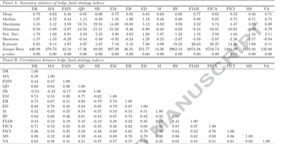
Our sample covers the period January 1994 to December 2013 (240 observations). This period includes a number of crises and market events which affected hedge funds returns, and caused large variability in the return series. The initial estimation period is January 1994 to December 2003 (120 observations), while the out-of-sample forecast period is January 2004 to December 2014 (120 observations). Summary statistics for the hedge fund return series are reported in Table 1. Panel A reports descriptive statistics for the different hedge fund strategies for the full sample of 240 observations. Quite interestingly, hedge fund strategies exhibit quite diverse statistical characteristics. All strategies (with the exception of SB) have a positive mean return ranging from 0.46% (EMN) to.0.85% (QD and EH). Event driven strategies (ED, DR, MA) are among the top performers, while equity hedge strategies are the most diverse ones. The average performance of the relative value indices is in a narrow band between 0.53% (FICI) and 0.77% (FIAB). Both EM and M indices are decent performers with mean returns of 0.75% and 0.63% respectively. Median returns are generally greater than mean returns with the exception of SB, M and EMN. Consistent with this finding, all strategies, with the exception of SB and M, exhibit negative skewness. The most skewed category is the relative value one and especially the FIAB index that has a skewness statistic of -3.50. Similarly, this category is the most leptokurtic one followed by the event driven one. The most volatile indices belong to the equity hedge (QD, SB) and emerging markets category (EM), while the strategies with the lowest volatility are the MA, EMN and FIAB. As expected, the null hypothesis of normality is strongly rejected in all cases.
Panel B reports pair-wise correlations between the hedge fund return series. The SB strategy is negatively correlated with all other strategies, but otherwise the correlations are all positive. The positive correlations range from 0.12 (between MA and FIAB) to 0.92 (between EH and QD). The indices that belong to the even-driven category exhibit correlations that vary between 0.59 and 0.88. The most diverse correlation pattern comes from the equity hedge families, as correlations vary from -0.86 for the QD-SB pair to 0.92 for the QD-EH pair. Overall, the relatively moderate pair-wise correlations suggest that benefits may accrue from the construction of funds of hedge funds.
[TABLE 1 AROUND HERE]
We model hedge fund returns by using an extensive list of information variables/ pricing 5For a detailed analysis of hedge fund styles and their risk-return characteristics, please refer to Bali et al.
factors along the lines of Agarwal and Naik (2004), Fung and Hsieh (2001, 2004), Vrontos et al. (2008), Meligkotsidou et al (2009), Wegener et al. (2010), Olmo and Sanso-Navarro (2012) etc. Our first set of explanatory factors for describing the hedge fund returns consists of the Fung and Hsieh factors, which have been shown to achieve considerable explanatory power. These factors are five trend-following risk factors which are returns on portfolios of lookback straddle options on bonds (BTF), currencies (CTF) commodities (CMTF), short-term interest rates (STITF) and stock indices (SITF) constructed to replicate the maximum possible return on trend-following strategies in their respective underlying assets. Fung and Hsieh also consider two equity-oriented risk factors, namely the S&P 500 return index (SP500), the size spread factor (Russell 2000 minus S&P 500), the bond market factor (change in the 10-year bond yield), the credit spread factor (change in the difference between Moodys BAA yield and the 10-year bond yield), the MSCI emerging markets index (MEM), and the change in equity implied volatility index (VIX).6 The next set of factors we consider are related to style investing and to investment policies that incorporate size and value mispricings. Specifically, we employ the HML (High minus Low) and SMB (Small minus Big) Fama-French factors along with the risk free interest rate (RF). Accounting for the fact that hedge fund managers might deploy trend-following and mean-reversion investment strategies, we also employ the Momentum (MOM), the Long Term Reversal (LTR) and the Short Term Reversal (STR) factor.7
Following Wegener et al. (2010) among others, we enhance our set of predictors with macro related / business indicators variables. Specifically, we employ the default spread (difference between BAA- and AAA-rated corporate bond yields), the term spread (10-year bond yield mi-nus 3-month interest rate), the inflation rate (INF) along with its one-month change (D(INF)), the US industrial production growth rate (IP), the monthly percent change in US non farm payrolls (PYRL), the US trade weighted value of the US dollar against other currencies (US-DTW) and the OECD composite leading indicator (OECD).8 We also employ some additional market-oriented factors; namely the Goldman Sachs commodity index (GSCI), the Salomon Brothers world government and corporate bond index (SBGC), the Salomon Brothers world government bond index (SBWG), the Lehman high yield index (LHY), the Morgan Stanley Capital International (MSCI) world excluding the USA index (MXUS) and the Russell 3000 (RUS3000) equity index.9 Finally, to proxy for market liquidity,we employ the Pastor and Stambaugh (2003) aggregate monthly innovation in liquidity measure (LIQ).10
6
The trend following factors are available at David Hsieh’s data library at
http://faculty.fuqua.duke.edu/˜dah7/DataLibrary/TF-FAC.xls. Data sources for the remaining factors are available there too.
7
For further details and data downloaad please consult the website of Professor Kenneth French at http://mba.tuck.dartmouth.edu/pages/faculty/ken.french/
8
The source of this set of factors is the FREDII database with the exception of the OECD leading indicator that was sourced from the OECD stats extracts.
9
The source of this set of factors is DATASTREAM International.
10
3.2 Statistical Evaluation of Forecasts
In our application, the natural benchmark forecasting model is the AR(1) model, which coincides with the linear regression model (1) when only the lagged hedge fund return is included in the model. As a measure of forecast accuracy we employTheil’s U,which is defined as
Theil’s U = M SF Ei
M SF EAR(1)
(7)
where M SF Ei is the Mean Square Forecast Error (MSFE) defined as the average squared forecast error over the out-of-sample period of any of our competing models and specifications andM SF EAR(1) is the respective value for the AR(1) model. Values less than 1 are associated with superior forecasting ability of our proposed model/specification and vice-versa.
3.2.1 Univariate models
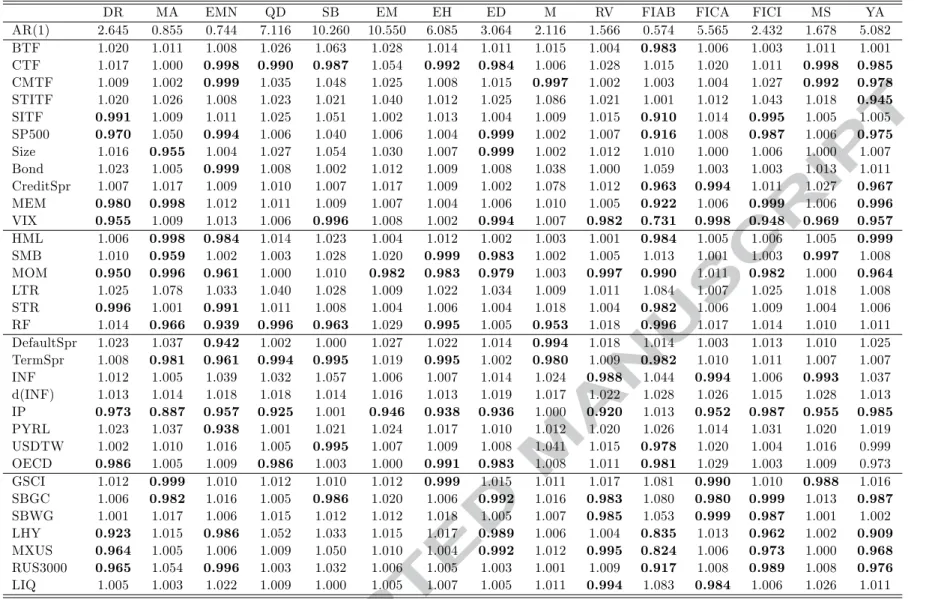
We start our analysis with the univariate models (Equation 1) by which we assess the forecasting ability of each one of the factors for the hedge fund strategies at hand. Table 2 reports the relatedTheil’s U values. As already mentioned values lower than 1 indicate superior predictive ability. Overall, we find considerable heterogeneity with respect to both the predictive ability of the candidate factors and the predictability of hedge fund strategies. Specifically, only two out of 32 factors do not improve forecasts over the benchmark for any of the hedge fund strategies under scrutiny. These are the long term reversal factor and the change in inflation. Quite interestingly, the most powerful predictor is the industrial production as it improves forecasts in 12 out of 15 hedge fund strategies followed by the momentum factor that helps predicting the returns of 10 strategies. This finding is line with Bali et al. (2014) who find that exposure to macroeconomic risk is a more powerful determinant than is the exposure to financial risk commonly used to explain hedge fund returns. VIX improves predictions in 9 strategies, while CTF, RF, term spread and SBGC are helpful at forecasting 7 strategies. The SP500, LHY and MXUS rank fifth as they are associated with improved predictive ability in 6 strategies.
Considering the predictability of hedge fund strategies, the most easily predicted strategies are FIAB (16 factors), EMN (14 factors) and YA (14 factors), DR (11 factors), ED (11 factors) and FICI (11 factors) followed by MA (10 factors). Eight factors improve forecasts of EH, RV and FICA, while seven factors improve forecasts for MS. More importantly, only 2 and 4 candidate predictors can improve forecasts of the EM and M strategies, respectively.
[TABLE 2 AROUND HERE]
In more detail, event driven strategies (ED, DR, MA) are mainly predicted by equity oriented factors, bond related factors (high-yield bond factor), momentum factors and business cycle related factors. This is quite expected as event driven strategies involve, implicitly or explicitly,
the risk of deal failure and/or financial distress. Their profitability depends on the outcome and timing of corporate events. When markets are down, volatility is up, bond yields increase, economic conditions deteriorate and naturally a larger fraction of deals fail. On the other hand, when markets are up, uncertainty is low and economic prospects improve, a larger proportion of deals go through and these strategies make profits. The predictive ability of the HML and SMB factors for the MA strategy is not surprising as smaller firms and/or high book-to-market ratio firms are more likely to be in distress. Moreover, both HML and SMB contain information related to news about future economic growth (Vassalou, 2003).11 These findings are consistent with previous studies; see for example Mitchell and Pulvino (2001), Agarwal and Naik (2004), Meligkotsidou and Vrontos (2008), Meligkotsidou et al. (2009).
Turning to the relative value group of strategies (RV, FIAB, FICA, FICI, MS and YA) we observe that the volatility index (VIX) appears to be the most important predictor for these style returns. This is expected as these strategies identify profit opportunities surrounding risk-adjusted price differentials between financial instruments and these price differentials are more likely to exist during periods of high volatility. Furthermore increased volatility can create relative value spreads that these strategies could exploit. Similarly to the ED family of hedge funds, the predictive ability of the industrial production is not surprising as current economic conditions signal future investment opportunities. This result is also consistent with the literature as the flattening or steepening of the yield curve depends on macroeconomic factors, like inflation, GDP growth and the monetary policy pursued by central banks and thus the fund manager’s macroeconomic view affects the fixed income arbitrage strategies employed. The group of bond factors, namely SBGC, SBWG, LHY appear significant for the majority of the RV strategies as these funds include fixed income securities including government and corporate bonds in both US and non-US markets. Moreover, past performance, captured by the momentum factor, and current equity market conditions (SP500 and RUS3000) improve forecasts for FIAB, FICI and YA strategies. It is worth noting that both the currency and commodity trend following factors improve forecasts for the MS and YA strategies that include in their portfolios non fixed income investments. Finally, the significance of the liquidity factor for both the RV aggregate and the FICA index points to the illiquid and infrequent trading nature of the financial instruments involved in these strategies.
With respect to the equity hedge indices, three factors, namely the currency trend following factor, the short-term interest rate and the term spread, are found to be useful predictors across all sub-strategies. The currency factor points to the international investment profile of this type of funds, while both the short-term interest rate and the term spread signal future economic activity and the concomitant stock market growth. Excluding these common factors, EH sub-strategies exhibit varying degrees of predictability ranging from 2 additional predictors for QD to 10 additional predictors for EMN. In line with Billio et al. (2012), Patton (2009) and
Meligkotsidou et al. (2009) who found that EMN funds are not market neutral, equity oriented factors, such as SP500, HML, MOM, STR and RUS3000, improve EMN predictability. On the other hand, the predictive ability of industrial production and the OECD leading indicator for QD shows significant exposures to business cycle risks.
Finally, the difficulty in characterizing both Macro and Emerging Markets strategies due to their broad investment mandate is clearly depicted in our forecasting results. For the Macro strategy, only business cycle related variables (indicators) such as the term spread, the default spread and the short-term interest rate variables along with the currency trend following factor improve forecasts. This finding is not surprising as macro fund managers employ commonly top-down approaches anticipating movements in macroeconomic variables and the impact of these movements on global financial markets. On the other hand, current economic conditions, as depicted by the industrial production, and past equity performance (momentum) turn out to be the only factors affecting future emerging markets hedge funds.
3.2.2 Combination of Forecasts
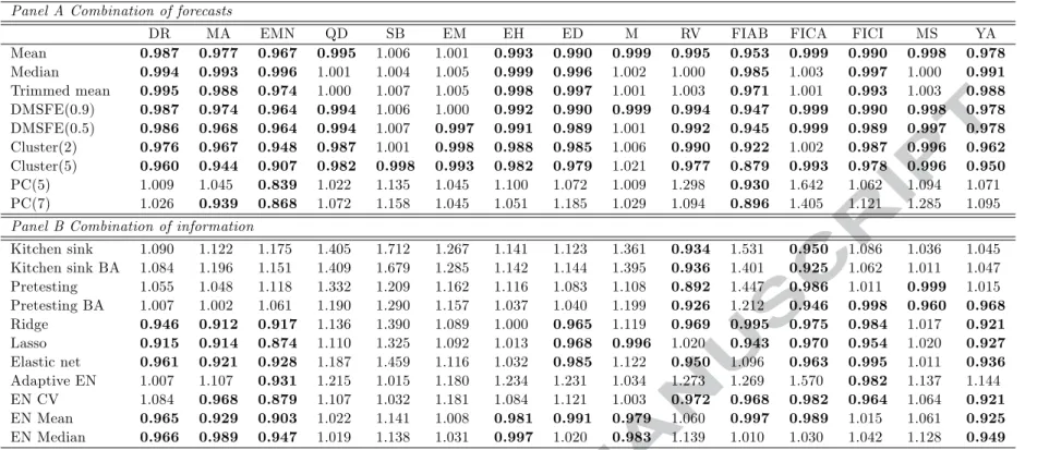
Table 3 (Panel A) reports our findings with respect to the predictive ability of the forecast combination schemes. Overall, our findings point to a quite robust picture as for the majority of hedge fund strategies, our forecast combination methods display MSFE ratios lower than 1 and thus improve on the ability of the AR(1) model to forecast each strategy. With the exception of the Principal Components methods, all the combining schemes improve forecasts for the event-driven strategies (ED, MA, DR), the equity hedge (total) strategy and two relative value strategies, namely the FICI and the YA strategy. It is worth mentioning that the EMN and FIAB strategies are the ones for which all the combining methods appear superior to the benchmark. On the other hand, SB, EM and M are the ones for which only less than three combining methods can beat the benchmark. For the remaining strategies, the mean, DMSFE and Cluster combining schemes improve forecasts. More importantly, the simplest forecasting schemes, i.e. the mean, is the best performer as it improves forecasts for thirteen out of fifteen strategies. The lowest MSFE ratios are associated with the Cluster(5) combining schemes which classifies the predictors in 5 clusters and forms forecasts on the basis of the best performing cluster. In the few cases (3 out of 15) that the PC methods display superior predictive ability over the AR(1) benchmark, their performance is associated with quite low MSFE ratios. For example, the MSFE ratios for the EMN strategy and the PC methods are as low as 0.84, while for the FIAB strategy and the PC(7) method the relative value is 0.896.
[TABLE 3 AROUND HERE]
3.2.3 Combination of Information
Table 3 (Panel B) displays our findings for the combining information approach. Overall, we observe considerable heterogeneity with respect to the ability of the respective methods to improve forecasts over the AR(1) benchmark. Both Kitchen Sink methodologies along with adaptive EN appear the weakest methodologies in our setting. Their forecasting ability is associated with only two strategies, namely either the RV and FICA (Kitchen Sink) or EMN and FICI (Adaptive EN). Pretesting and Pretesting with bagging seem to work better, as these methods offer improved forecasts for 3 and 5 strategies, respectively. The Lasso, Ridge and mean Elastic Net specifications offer further improvement (9 strategies). Among the Elastic Net variants employed in this study, the adaptive Elastic Net, despite its computational intensity, performs worse since it only displays superior ability for the EMN and FICI strategy. Six strategies, namely QD, SB, EM, EH, M and MS appear hard to forecast, while FICA seems to be the one favoured by these methods. For the remaining strategies, forecast improvements depend on the choice of method. For example, DR, MA, EMN, FICI and YA, broadly favour the Ridge, Lasso and Elastic Net specifications, while RV favours the Kitchen sink, pretesting and bagging methods.
Overall, when comparing Panels A and B, the combination information methodologies seem inferior to the combination forecasts schemes at least from a statistical point of view. To this end, we assess whether the same picture pertains when the economic value of our forecasts is assessed.
3.3 Economic Evaluation
3.3.1 The framework for economic evaluation
As Campbell and Thompson (2008) and Rapach et al. (2010) suggest, even small reductions in MSFEs can give an economically meaningful degree of return predictability that could result in increased portfolio returns for a mean-variance investor that maximizes expected utility. Within this stylized asset allocation framework, this utility-based approach, initiated by West et al. (1993), has been extensively employed in the literature as a measure for ranking the performance of competing models in a way that captures the trade-off between risk and return (Fleming et al., 2001; Marquering and Verbeek, 2004; Della Corte et al. 2009, 2010; Wachter and Warusawitharana, 2009).
Consider a risk-averse investor who constructs a dynamically rebalanced portfolio consisting of the risk-free asset and one risky asset. Her portfolio choice problem is how to allocate wealth between the safe (risk-free Treasury Bill) and the risky asset (hedge fund strategy), while the only source of risk stems from the uncertainty over the future path of the respective hedge fund index. Since only one risky asset is involved, this approach could be thought of as a standard exercise of market timing in the hedge fund industry. In a mean-variance framework,
the solution to the maximization problem of the investor yields the following weight (wt) on the risky asset
wt=
Et(rt+1)
γV art(rt+1)
(8) where Et and V art denote the conditional expectation and variance operators, rt+1 is the
return on one of the hedge fund strategies considered and γ is the Relative Risk Aversion (RRA) coefficient that controls the investor’s appetite for risk (Campbell and Viceira, 2002; Campbell and Thompson, 2008; Rapach et al., 2010). The conditional variance of the portfolio is approximated by the historical variance of hedge fund returns and is estimated using a 5-year rolling window of monthly returns.12 In this way, the optimal weights vary only with the degree the conditional mean varies, i.e. the forecast each model/ specification gives. Under this setting the optimally constructed portfolio gross return over the out-of-sample period, Rp,t+1,is equal
to
Rp,t+1=wt·rt+1+Rf,t
whereRf,t= 1 +rf,t denotes the gross return on the risk-free asset from periodttot+ 1.13 Assuming quadratic utility, over the forecast evaluation period the investor with initial wealth of W0 realizes an average utility of
U = W0 (P −P0) P−P0−1 X t=0 (Rp,t+1− γ 2(1 +γ)R 2 p,t+1) (9)
whereRp,t+1is the gross return on her portfolio at timet+1.14At any point in time, the investor
prefers the model for conditional returns that yields the highest average realized utility. Given that a better model requires less wealth to attain a given level of U than an alternative model, a risk-averse investor will be willing to pay to have access to this superior model which would be subject to management fees as opposed to the simple HA (historical average) model. In the event that the superior model is one of our proposedispecifications, the investor would pay a performance fee to switch from the portfolio constructed based on the historical average to the
i specification. This performance fee, denoted by Φ, is the fraction of the wealth which when subtracted from the iproposed portfolio returns equates the average utilities of the competing models. In our set-up the performance fee is calculated as the difference between the realized
12See Campbell and Thomson (2008) and Rapach et al. (2010). 13
We constrain the portfolio weight on the risky asset to lie between 0% and 150% each month, i.e. 0≤wt≤1.5.
14One could instead employ other utility functions that belong to the constant relative risk aversion (CRAA)
family such as power or log utility. However, quadratic utility allows for nonormality in the return distribution while remaining in the mean-variance framework.
utilities as follows: 1 (P−P0) P−P0−1 X t=0 (Rp,ti +1−Φ)− γ 2(1 +γ)(R i p,t+1−Φ)2 = (10) 1 (P−P0) P−P0−1 X t=0 RHAp,t+1− γ 2(1 +γ)(R HA p,t+1)2 .
If our proposed model does not contain any economic value, the performance fee is negative (Φ≤0),while positive values of the performance fee suggest superior predictive ability against the HA benchmark. We standardize the investor problem by assumingW0 = 1 and report Φ in
annualized basis points.
3.3.2 Economic evaluation findings
We assume that the investor dynamically rebalances her portfolio (updates the weights) monthly over the out-of-sample period employing the forecasts given by our approaches. Similarly to the statistical evaluation section, the out-of-sample period of evaluation is 2004:1-2013:12. The benchmark strategy against which we evaluate our forecasts is the naive historical average model. For every specification we calculate the performance fee from Equation (10) setting RRA (γ) equal to 3. Table 4 reports the respective findings.
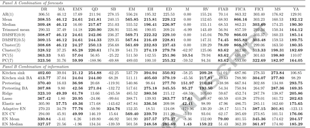
[TABLE 4 AROUND HERE]
The first line (AR(1)) of Table 4 corresponds to the performance fee an investor would pay to have access to the simple AR(1) model. Given the significant autocorrelation of hedge fund returns, it is not surprising that Φ ranges from 0 bps (M strategy) to 863 bps (FICA). Even with this simple model an investor can enjoy gains of up to 8.6%. While the majority of strategies point to gains greater than 100 bps, the MA, EMN and FIAB strategies generate lower, albeit positive, profits.
With respect to our proposed methodologies, the most striking feature of Table 4 is the gen-eration of positive gains that exceed the ones generated by the AR(1) model for every strategy considered. However, consistent with our statistical evaluation findings, forecast combination methods seem to perform better than combination information methods, by a narrow margin though. For example, the Adaptive elastic net method that hardly generated improved fore-casts statistically, exceeds the performance of the AR(1) model in four strategies, among them the SB for which no other methodology succeeds in it. Similar improvements prevail for the Kitchen sink and BA methodologies that were found statistically inferior to forecast combi-nation methods. Overall, an investor that bases her forecasts on simple combining schemes (mean, median, trimmed mean) always generates positive profits, while the chances of expe-riencing losses increase if forecasts are generated on the basis of combination of information methods.
4
Dynamic Hedge Fund Portfolio Construction
In this section, we examine the benefits of introducing hedge fund return predictability in hedge fund portfolio construction and risk measurement. This is achieved through an investment exercise which compares the empirical out-of-sample performance of our forecasting approaches. Section 4.1 sets out the optimization framework and Section 4.2 the portfolio evaluation criteria. Section 4.3 reports our findings for various types of investors and portfolio optimization methods. 4.1 Optimization framework
Consider an investor who allocates her wealth amongn= 15 hedge fund indices with portfolio weight vectorx= (x1, x2, ..., xn)0.While several approaches to constructing optimal portfolios exist, the most common (standard) is the mean-variance model of Markowitz (1952), in which the risk measure is the portfolio variance. Given that our methodology is focused on the benefits of return predictability for asset allocation, the variance of the portfolio of hedge funds returns is approximated by the sample covariance matrix.
More in detail, in the mean-variance framework, portfolios are constructed through the following optimization scheme
minV ar(rp) (11) s.t. xL≤xi ≤xU, i= 1, ..., n, n X i=1 xi= 1, and E(rp)>rG,
whererpis then−assets portfolio return,x= (x1, x2, ..., xn)0 is the vector containing the assets’ weights in the portfolio, E(rp) and V ar(rp) = x0Vx are the expected return and the variance of the portfolio, respectively, V is the n×n sample covariance matrix of the returns, and rG is the target portfolio return. Given that currently short selling hedge fund indices does not represent an investment tactic, portfolio weights are constrained to be positive (i.e. the lower bound of weights, xL,is set equal to 0).In order to facilitate diversification, we set the upper bound of portfolio weights equal to 0.50 (xU = 0.50,see also Harris and Mazibas, 2013). This setup represents a conservative investor who is primarily concerned with the risk he undertakes. The following more general framework can accommodate varying degrees of investor appetite for risk. Specifically, we also construct portfolios through the following optimization scheme
min λV ar(rp)−(1−λ)E(rp) (12) s.t. xL≤xi ≤xU, i= 1, ..., n, n X i=1 xi= 1, and E(rp)>rG,
for various values of the risk appetite parameter λ, λ ∈[0,1]. For the case of λ= 1,we obtain the minimum variance optimization scheme (11). We setλequal to 0.50, 0.25 and 0. The case
of λ= 0 represents an aggressive investor that is primarily interested in maximizing returns, employing the following optimization scheme:
max E(rp) (13) s.t. xL≤xi≤xU, i= 1, ..., n, n X i=1 xi= 1, andV ar(rp)6φ, whereφ is the upper allowed level of portfolio variance.
Finally, we consider controlling for risk objectives such as the portfolio Conditional Value at Risk (CVaR) along the lines of Krokhmal et al. (2002). The CVaR is a risk measure defined as the expectation of the losses greater than or equal to the Value at Risk (VaR), which measures the risk in the tail of the loss distribution.15 The mean-CVaR optimization problem is expressed mathematically as follows minCV aR(Frp, α) (14) s.t. xL≤xi ≤xU, i= 1, ..., n, n X i=1 xi= 1, and E(rp)>rG, with CVaR(Frp, α) =−E(rp|rp ≤ −VaR) =− R−VaR −∞ zfrp(z)dz Frp(−VaR) , (15)
wherefrp andFrp denote the probability density and the cumulative density ofrp, respectively,
αis a probability level, and VaR(Frp, α) =−F
−1
rp (1−α). We employ Rockafellar and Uryasev’s
(2000) convex programming formulation. Rockafellar and Uryasev (2002) provide a thorough discussion of the properties of CVaR in risk measurement and portfolio optimization exercises. 4.2 Evaluation criteria
Similarly to the forecast evaluation (Section 2), the performance of the constructed portfolios is evaluated over the out-of-sample period using a variety of performance measures. Each portfolio is rebalanced monthly and the realized portfolio returns are calculated at the rebalancing date given the optimized weights.
First, we consider the realized returns of the constructed portfolios. Given the portfolio weights xt= (x1, x2, ..., xn)0t at time t and the realized returns of the n assets in our sample at time t+ 1, rt+1 = (r1, r2, ..., rn)0t+1, the realized return rp of the portfolio at time t+ 1 is computed as
rp,t+1 =x0trt+1.
15Bali et al. (2007) find evidence of a positive and significant link between VaR and hedge fund returns in the
We calculate the average return (AR) within the out-of-sample period and the cumulative return at the end of the period. We also calculate the end period value (EPV) of our portfolio at the end of the out-of-sample period for a portfolio with investment of 1 unit at the beginning of the out-of-sample period.
Next, we consider measures related to risk, i.e. we report and discuss the conditional volatil-ity of the portfolio determined by each different mean/covariance model, which is computed as
p
V ar(rp) = √
x0Vx. Due to the fact that portfolio optimization schemes generally arrive at a different minimum variance for each prediction model, the realized return is not comparable across models since it represents portfolios bearing different risks. Therefore, a more appro-priate/realistic approach is to compare the return per unit of risk. In this sense, we use the Sharpe Ratio (SR) which standardizes the realized returns with the risk of the portfolio and is calculated through SRp = E(rp)−E(rf) p V ar(rp) ,
where rp is the average realized return of the portfolio over the out-of-sample period, and
V ar(rp) is the variance of the portfolio over the out-of-sample period.
A portfolio measure associated with the sustainability of the portfolio losses is the maxi-mum drawdown (MDD) which broadly reflects the maximaxi-mum cumulative loss from a peak to a following bottom. MDD is defined as the maximum sustained percentage decline (peak to trough), which has occurred in the portfolio within the period studied and is calculated from the following formula
M DDp = max
T0≤t≤T−1[T0≤maxj≤T−1(P Vj)−P Vt],
whereP V denotes the portfolio value andT0, T denote the beginning and end of the evaluation
period, respectively.
The next three measures we calculate, namely the Omega (OMG), Sortino (SOR) and Upside Potential (UP) ratios, treat portfolio losses and gains separately. In order to define these measures, we first define the n-th lower partial moment (LP Mn) of the portfolio return as follows (see Harlow, 1991; Harlow and Rao, 1989 and Sortino and van der Meer, 1991) :
LP Mn(rb) =E[((rb−rp)+)n]
whererb is the benchmark return and the Kappa function (Kn(rb)) is defined as follows:
Kn(rb) = E(rp)−rb n p LP Mn(rb) .
Then the respective measures are calculated as follows:
OM G(rb) =K1(rb) + 1, SOR(rb) =K2(rb), U P(rb) =
E[(rp−rb)+]
p
LM P M2(rb)
Next, we set out to incorporate transaction costs. Transaction costs associated with hedge funds, however, are not generally easy to compute given the variation in early redemption, management or other types of fees (Alexander and Dimitriu, 2004). Nevertheless, if the gain in the performance does not cover the extra transaction costs, less accurate, but less variable weighting strategies would be preferred. To study this issue we define portfolio turnover (PT) as (Greyserman et al., 2006): P Tp = T−1 X t=T0 n X i=1 |xi,t+1−xi,t|
Finally, we investigate the capacity of the different prediction models to assess tail-risk. A CVaR ofλ% at the 100(1-α)% confidence level means that the average portfolio loss measured over 100α% of worst cases is equal toλ% of the wealth managed by the portfolio manager. To compute CVaR, we use the empirical distribution of the portfolio realized returns. CVaR is calculated at the 90%, 95%, and 99% confidence levels.
4.3 Empirical Results
In this section, we report the out-of-sample performance of our optimization procedures and the proposed forecasting methodologies. The evaluation period is the same with the one employed for the statistical and economic evaluation of forecasts, i.e. January 2004 to December 2013. We construct portfolios in a recursive manner starting in January 2004 and employing the related return forecasts. We calculate buy-and-hold returns on the portfolio for a holding period of one month and then rebalance the portfolio monthly until the end of the evaluation period. As aforementioned, the hedge fund portfolios are constructed based on two optimization techniques, themean-variance and themean-CVaR.We report the performance of the forecast combination and information combination approaches along with the naive (equally weighted) portfolio and the HFR fund of hedge funds index. We set an annual target return, rG = 12%, in the optimization schemes used and employ the US 3-month interest rate for the risk free rate and for the benchmark rate of return (rb) necessary for the calculation of OMG, MDD and SOR.16
For the mean-variance optimization framework, we consider four types of investor by varying the degree of risk appetite through the parameterλ. Usingλ= 1 penalizes more the risk of the
16
Please note that the target return is not always achieved by the optimization procedure. In these cases, the target is lowered to the highest possible value, i.e. 11%, 10%, etc. Harris and Mazibas (2013) set a target return of 14% in their optimization procedure.
constructed portfolio and results in aminimum variance portfolio with a specific target return. Thus, inherent in the portfolio construction is an additional constraint that the mean portfolio return should be greater than or equal to the target valuerG. Usingλ= 0.50 penalizes less the risk of the constructed portfolio and could be suitable for a medium risk averse fund manager. Furthermore, usingλ= 0.25 describes the risk profile of a more aggressive fund manager while considering λ= 0 reduces to the optimization scheme of maximizing expected return. In this portfolio the upper allowed level for the portfolio variance is set at φ= 2.5% monthly.
In the above portfolio optimization procedures we consider different restrictions on the weights of the constructed portfolios; at first, we restrict the weights to be greater than zero and smaller than 0.50, i.e. 0 ≤xi ≤ 0.50, i= 1, ..., n, that is short selling is not allowed. We also examine the case that short selling is allowed, using −0.5 ≤ xi ≤ 0.5 in our portfolio exercise. Thus, we examine the robustness/sensitivity of the constructed portfolio performance to different restrictions of portfolio weights. Allowing for short-selling enables us to benefit from the forecasting ability of the proposed methodologies in the case of negative future returns.
Second, we consider a mean-CVaR portfolio optimization approach, which involves con-structing optimal portfolios by minimizing the Conditional Value at Risk (CVaR) employing the empirical distribution of asset returns based on the approach of Rockafellar and Uryasev (2002). In this optimization scheme, we also employ an additional constraint that the mean portfolio return should be greater than or equal to the target value rG. The confidence level used is set at 95% and 99%.
Minimum variance (λ= 1)
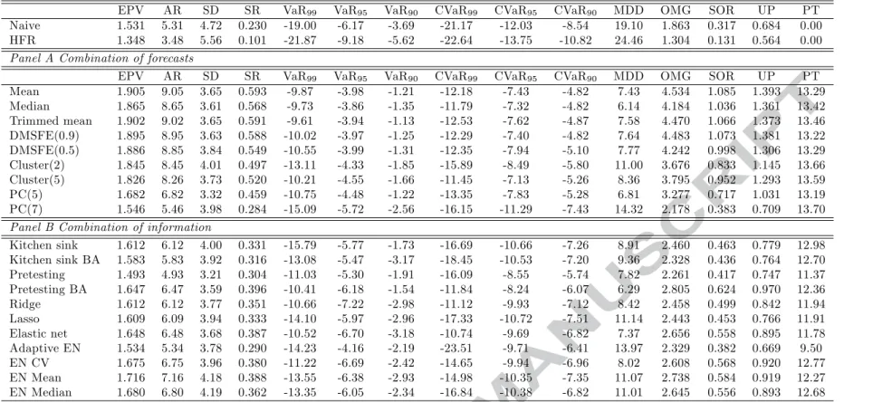
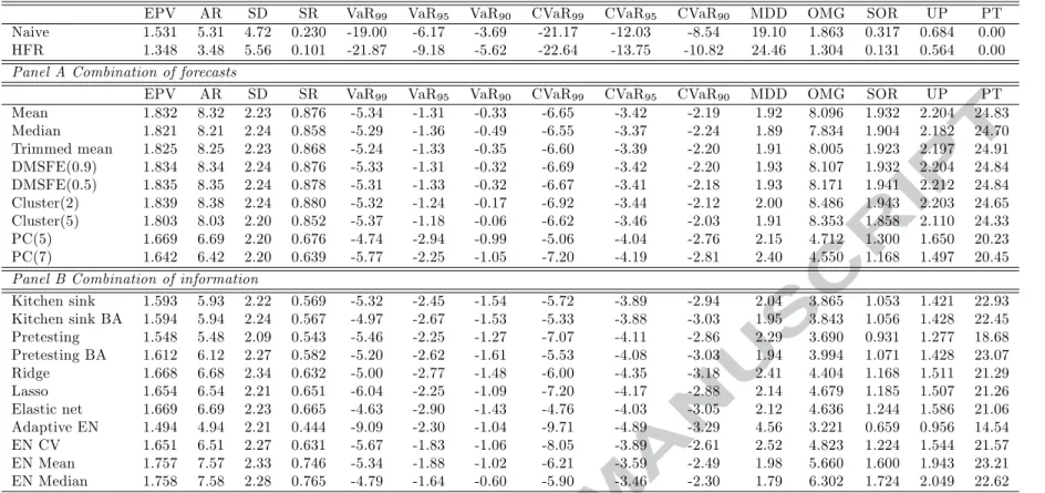
Table 5 reports the results for the minimum variance investment strategy. The best performing forecasting methods, according to the majority of the performance measures are the Mean, the Trimmed mean and the DMSFE (0.9). These model portfolios have the largest average returns, ranging from 8.95% to 9.05%, as well as the highest Sharpe Ratios (0.588 to 0.593). They also have the highest Omega, Sortino and Upside values. It is worth mentioning that the naive strategy attains an average return of 5.31%, associated with high volatility resulting in a Sharpe ratio of 0.230. As expected, the performance of this strategy is associated with lower values of Omega, Sortino and Upside measures. Turning to the HFR fund of funds portfolio, we observe that its performance is inferior to the naive strategy. It attains an average return of 3.48% and a Sharpe ratio of 0.101 due to increased volatility. While the combination of information methods appear superior to the naive and HFR strategies, they lack in performance when compared to the combination of forecasts approaches (with the exception of the PC(7) method).
[TABLE 5 AROUND HERE] Mean-variance (λ= 0.50)
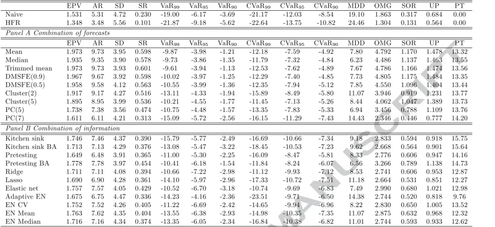
Table 6 reports the results for the first formulation of the mean-variance investment strategy, which corresponds to a medium risk averse investor. Our findings are similar in spirit to the ones
reported for the minimum variance investment strategy. Overall, the combination of forecasts methods (with the exception of the PC methods) rank first having an average return that exceeds 8.95%. These approaches have the highest Sharpe ratios, ranging from 0.536 to 0.598. Furthermore, the least volatile method is the PC(5) method. Finally, we should note that portfolio turnover is quite similar across the forecasting approaches except for the Adaptive Elastic Net that displays a much lower portfolio turnover.
[TABLE 6 AROUND HERE] Mean-variance (λ= 0.25)
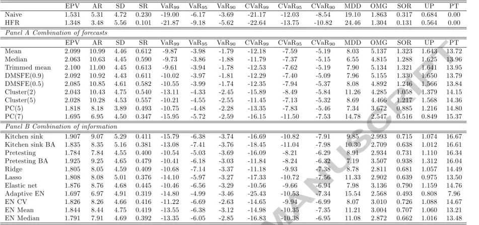
The results associated with the more aggressive mean-variance formulation are reported in Table 7. As expected, our forecasting approaches generate higher returns compared to the investment strategies considered so far. Quite interestingly, these gains are not associated with significant increases in the portfolios’ risk and as such we observe increases in the Sharpe, Omega, Sortino and upside ratios. The maximum drawdown, VaR and CVaR measures improve (decrease) as well. The ranking of the methods remains broadly unchanged with the best performing methods being the Mean, Trimmed Mean and DMSFE(0.9) combination methods.
[TABLE 7 AROUND HERE] Maximizing expected return (λ= 0)
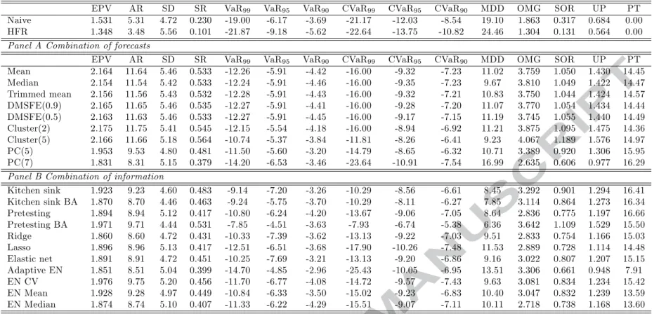
Maximizing expected return is the investment strategy more related to the mean forecasting experiment we conduct. Our findings (reported in Table 8) suggest that the best performing methods are the forecast combination ones (with the exception of PC methods), although improved performance is attained for all the methods at hand. As such, average returns range from 8.31% (PC(7)) to 11.75% (Cluster(2)). Since this strategy is riskier than Cluster(5), the highest Sharpe ratio (0.564) is achieved by the Cluster(5) combination method. Moreover, portfolio turnover is in general lower for the forecast combination methods than the combination of information ones (with the exception of the Adaptive EN, EN Mean and EN Median).
[TABLE 8 AROUND HERE] Minimum-variance (λ= 1)− Shortselling allowed
Relaxing the short-selling restriction offers some interesting insights with respect to the risk return profile of the formed portfolios. Our findings with respect to the minimum-variance portfolio, reported in Table 9, point to non significant gains in terms of average returns compared to the long only portfolio (Table 5). However, the low risk profile of this strategy is enhanced leading to significant reductions in volatility. The standard deviation of the portfolios ranges from 2.09% to 2.34% as opposed to values ranging from 3.21% to 4.19% for the long-only case. As such, Sharpe ratios appear increased and reach the value of 0.880 for the Cluster 2 method,
while the maximum drawdown hovers around 2.5% (with the exception of the Adaptive EN). Quite interestingly, the differences in the performance of the forecasting approaches appear to have phased out.
[TABLE 9 AROUND HERE]
Figure 1 summarizes the relation between the risk aversion parameter λ (for λ= 0, 0.25,
0.50, 0.75, 1) and portfolio performance variables, such as the average return, the standard deviation, the Sharpe and Sortino ratio for a selection of forecasting methodologies. Average returns decline for all the methodologies at hand as we move from an aggressive investor portfolio to a conservative one. Similarly, volatility decreases as risk aversion increases with the exception of the Kitchen Sink BA and Pretest BA forecasts where an increase is prevalent forλ= 0.25.
Turning to the Sharpe ratio figure, we have to note that Sharpe ratios decline slightly with λ,
except for a spike at λ= 0.25 for the mean combining scheme. Finally, Sortino ratios largely follow the path of Sharpe ratios, i.e. they decrease withλ.As previously, an increase atλ= 0.25 is apparent for the mean, Cluster(2) and EN methods.
[FIGURE 1 AROUND HERE] Maximizing expected return (λ= 0)−Shortselling allowed
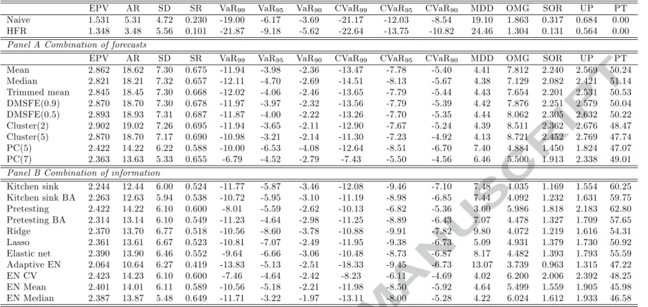
We now turn to the performance of theMaximizing expected return strategy when shortselling is allowed. The respective evaluation criteria are reported in Table 10. The most striking feature of Table 10 is the impressive average return, which exceeds 18% for the forecast combination methods except for the PC ones. However, irrespective of the method considered, average returns are higher than 10.64% (Adaptive EN model), while the best performing method is the Cluster(2) combination scheme with an average return of 19.02%. The elevated volatility of these portfolios leads to lower Sharpe ratios compared to the previous formulation, which in general are quite high and exceed 0.5. Quite interestingly, the maximum drawdown associated with the best performing methods are quite low at values ranging from 4.1% to 4.4%. Naturally, relaxing short selling increases portfolio turnover.
[TABLE 10 AROUND HERE] Mean CVAR α= 5%, α= 1%
Finally, we report the performance ofMean-CVaR optimal portfolios These results correspond to portfolios constructed through Equation (14) for a target return of 12% and for probability levels of 95% and 99%. Table 11 reports the results for the mean CVAR optimization scheme at a 95% confidence level. The best performing forecasting methods, according to the majority of the performance measures are the forecast combination methods with the exception of the PC ones. These model portfolios have the largest average returns, ranging from 9.25% to 10.36%, as well
as the highest Sharpe Ratios (0.344 to 0.432). They also have among the highest Omega, Sortino and Upside values. Table 12 reports the results for the mean CVAR optimization scheme at a 99% confidence level. The results are similar to the results of the mean CVAR optimization scheme at a 99% confidence level. The best performing forecasting methods, according to the majority of the performance measures are the the forecast combination methods with the exception of the PC ones. These model portfolios have the largest average returns, ranging from 9.37% to 10.47%, as well as the highest Sharpe Ratios (0.345 to 0.420). They also have among the highest Omega, Sortino and Upside values. Our findings are in line with Bali et al. (2007), who find that buying the higher VaR portfolio while short selling the low VaR portfolio generates an average annual return of 9% for the sample period of January 1995–December 2003.
[TABLES 11 & 12 AROUND HERE]
5
The 2007-2009 Crisis Period
The recent financial crisis period (2007-2009) was quite difficult for hedge funds as many hitherto successful hedge fund managers were hit with significant losses. Elevated credit, liquidity and systemic risk constitutes this period very different from the period prior to 2007 or after 2009. We would expect that the predictability patterns observed during normal periods may not appear during turbulent periods. In other words, factors useful in predicting returns during normal periods may not work during the crisis. To address this issue we repeat our analysis for the sub-period 2007-2009 corresponding to the recent financial crisis.
5.1 Statistical Evaluation 5.1.1 Univariate models
We start our analysis with the univariate models in order to assess the forecasting ability of each one of the factors for the hedge fund strategies at hand. Table 13 reports the related Theil’s U values. Overall, we find increased predictive ability of the candidate factors for all the hedge fund strategies at hand compared to our full sample. This finding is consistent with Rapach et al. (2010) who found that out-of-sample return predictability is notably stronger during business-cycle recessions vis-a-vis expansions.
While in the full sample, the most powerful predictor is the industrial production, during the crisis period, VIX emerges as equally powerful. Both variables improve forecasts in 13 out of 15 hedge fund strategies. This finding suggests that overall current economic conditions (proxied by IP) and