Intersectoral resource allocation and its impact on economic development in the Philippines

WeS 1883

POLICY

RESEARCH

WORKING

PAPER

18

8 3

Intersectoral Resource

a developing economy shifts

Allocation and Its Impact

on Economic Development

on E

Hconomic

Development

in the Philippines

discourage agriculture caused both the industrial and

Fumihide Takeuchi agricultural sectors to decline,

Takehiko Hagizno as conglomerates (landed

capitalists) made inefficient use of resources and exacerbated the already

uneven distribution of income.

The World Bank

Development Research Group

Public Disclosure Authorized

Public Disclosure Authorized

Public Disclosure Authorized

POLIcY RESEARCH WORKING PAPER 1883

Summary findings

For sustained growth, a developing economy must Philippines, however, the outcome of these policies was provide productive employment opportunities in unique. Measures designed to discourage agriculture, nonagricultural sectors. As the economy grows, rather than encourage the industrial sector, caused both employment shifts from the agricultural sector to it and the agricultural sector to deteriorate.

industrial and service sectors. Takeuchi and Hagino criticize financial conglomerates The move away from agriculture happens because of for creating highly oligopolistic market structures that the decline in the income elasticity of food as incomes were responsible for the inefficient use of resources and rise, the discovery of substitutes for agricultural unbalanced income distribution. Many of the

products, and rapid technological changes in agriculture conglomerates (dubbed "landed capitalists") channeled in response to shortages of land. massive state resources into such traditional economic

The economic policies developing economies pursue activities as sugar and coconut farming, limiting the are typically designed to accelerate this structural country's industrial diversification.

transformation by favoring the industrial sector. In the

This paper - a product of the Development Research Group - is part of a larger effort in the department to. Copies of

the paper are available free from the World Bank, 1818 H Street NW, Washington, DC 20433. Please contact Kari Labrie, room MC3-347, telephone 202-473-1001 fax 202-522-3518, Internet address klabrieaworldbank.org. February 1998. (31 pages)

The Policy Research Working Paper Series disseminates the findings of work in progress to encourage the exchange of ideas about development issues. An objective of the series is to get the findings out quickly, even if the presentations are less than fully polished. The papers carry the names of the authors and should be cited accordingly. The find isgs, interpretations, and conclusions expressed in this paper are entirely those of the authors. They do not necessarily represent the vnew of the World Bank, its Executive Directors, or the

Intersectoral Resource Allocation and Its Impact on Economic Development in the Philippines'

Fumihide TAKEUCHI Takehiko HAGINO

Japan Center for Economic Research

1. Stagnancy in the industrial structure in the Philippine economy

For sustained growth to be realized in developing economies, it is necessary that more productive employment opportunities in non-agricultural sectors be available to the people. And in order for economic growth in developing countries to be a

sustained growth, it is necessary that the country's non-agricultural sector is developed to the extent that it can provide these employment opportunities.

Both economic theory and modern economic history show that productivity growth in non-agricultural sectors has consistently outweighed that of the agricultural sector. Thus, as development progresses, employment, which had been centered around the agricultural sector, becomes more and more dependent on the industrial and services sectors. This relationship between economic growth, and the move away from agriculture can also be explained in terms of the decline in the income elasticity of food as incomes rise, the discovery of substitutes for agricultural products, and the rapid technological change in agriculture in response to shortages of land. Economic policies pursued by some developing economies are typically designed to accelerate this structural transformation by favoring the industrial sector.

In the case of the Philippines, however, the outcome of these policies has been quite unique. Measures towards industrialization that were designed to discourage agriculture did not drastically change the industrial structure, and rather than encouraging the industrial sector, led to the deterioration of industry, as well as agriculture. We can imply from this that there were non-market forces at work in

This paper was prepared for the Workshop entitled "Political Economy of Rural Development Strategies ", to be held on May 5-6 at the World Bank, Washington, DC.

The authors would like to acknowledge the contribution of the National Statistical Coordination Board, Banko Sentral ng Pilipinas (Central Bank of the Philippines) in collecting data.

the resource (capital and labor) allocation between agriculture and non-agriculture sectors.

Table 1 shows the changes in the sectoral composition of aggregate output and employment. Industry's share of GDP rose and agriculture's share fell, demonstrating a familiar pattern of development, but this change took place only from the mid-1950s to mid-1970s. In terms of employment, the share of those employed in industry failed to grow even in that period, suggesting that the service and agricultural industries were the major sources of employment. This stagnancy in the industrial structure is particularly noticeable when we make international comparisons (Table 2). Table 2(a) shows the percentage shares of agricultural output in total GDP from 1977 to 1990, and Table 2(b) shows those of the manufacturing industry from 1970 to 1990. The percentage decline in the share of agriculture over the period is only 9.6% and the percentage share of manufacturing in GDP did not change at all. This feature stands out even in comparison with other South Asian economies.

Some other important issues to be discussed are the efficiencies of resource utilization and income distribution. A transfer of capital out of agriculture will lead to sustained growth only if this is done efficiently towards more socially profitable investments coupled with a relatively balanced income distribution. Therefore, "balanced" intersectoral resource flows should be evaluated not only on the relative size of flows but also by these criteria.

In the case of the Philippines, the inefficient use of resources and the unbalanced income distribution seem to be as problematic as the relative size of intersectoral resource allocation. Some great financial conglomerates are criticized for creating highly oligopolistic market structures which are seen as responsible for the inefficient resource use and uneven income distribution. Many of them are "landed capitalists", and they have channeled massive state resources into traditional economic activities like sugar and coconut farming, lirniting the country's industrial diversification.

2. Capital Allocation Between the Agriculture and Non-Agriculture Sectors.

In this project, aggregated intersectoral resource allocation is estimated in each sample country using regional data (taking the "regional approach"); agricultural and non-agricultural regions are defined, and transfers from one to another is regarded as an intersectoral transaction. This approach is adopted as a convenient way to gauge intersectoral allocation.

However, classifying the regions into the two types of regions is difficult in some cases due to the ambiguity of the sectoral distribution of output and employment in many regions. In addition, the limited availability of data makes it difficult to cover all kinds of resource transactions and to compare private and public-based allocations on the same basis.

Thus, we try to estimate the capital allocation2 between the agricultural and non-agricultural sectors in two different ways: one is by taking the above-mentioned

regional approach and the other is a sectoral approach by using input-output tables.

In this discussion, our estimations using the sectoral approach covers intersectoral capital transfer between agricultural and non-agricultural sectors3 _{from 1961 to}

1982, when I-0 tables and government contributions data(taxes and subsidies) to capital transfers are available4.

Here, net real resources transferred from one sector to another and the financial contributions of one sector to another are, by construction, equal . Transferred net real resources (the trade balance) can be extracted from 1-0 tables and the financial contribution of one sector to another is equal to the net private flows [saving(S) less

2 We have not touched on the labor force allocation between the different sectors in this discussion.

The following estimation of intersectoral capital transfers also excludes factor returns (wvages). Regarding the labor force allocation between agriculture and industrv .the industrialization of the Philippines has been criticized by many as being extremely capital-intensive compared to other East Asian economies.

Under capital-intensive industrialization, Metro Manila and its peripheral areas limited labor absorption from the agricultural sector (rural regions), resulting in the stagnant industrial structure described above. Leon(1982) estimated the intersectoral capital flows as well as intersectoral labor flows and using these, found a capital/labor ratio in terms of flows. He discovered huge capital transfers from the agriculture to non-agriculture industries, coupled with a relatively small outflow of labor. This suggests an industrial structure biased in favor of capital-intensive projects and minimal growth in agricultural labor productivity.

3 Accounting framework and estimation procedures are based on Leon (1982), with slight modifications. See appendix.

4 1-0 tables are available for the years 1961, 65, 74. 79, 83. 85 and govermnent taxes and subsidies

to agriculture can be obtained for the years 1960-82 from the World Bank's survey (1990). Intersectoral capital flows are estimated by combining the two sources. Trade balances in-between 1-0 years are estimated as straight line extensions. Hence, we are able to obtain

intersectoral capital transfers from 1961 to 1982.

investment(I)] plus govermnent receipts [taxes(T)]5. The net real resources transferred from the agricultural to non-agricultural sectors are, for example, the difference between the food and raw materials del:ivered to the non-agricultural sector and the industrial consumer goods and indlustrial inputs flowing in the opposite direction.

Table 3 shows net capital outflows as a proportion of agricultural Gross Value Added. The column second from the left shows the marketed capital transfers (S-I+T) which can be directly obtained from the 1-0 tables. (S-I) equals the private based net capital outflows, and public based net capital outflows are represented by (T-G). The total net flows aggregated by these two (S-I+T-G) are shown separately.

As shown in table 3, the agricultural sector maintained net capital outflows to the non-agricultural sector over the course of the period. As for the public based transfers, the government spent more in agriculture than it gained from the taxation of the sector during most of the years surveyed. However, the government-led inflows were not sufficient to compensate for the privat:e based capital outflows. We can also see that a significant share of transfers out of agriculture occurred during the first half of 1970s6_.

Figure 1 indicates that the domestic agriculture to non-agriculture terms of trade (TOT) improved during the first half of the 1970s, which may be responsible for the relatively large capital outflows (equal to the surplus in the trade balance by definition) 7. TOT can affect the sectoral IS balance in a different way. TOT

5 To obtain total net capital balance (IS balance) of the agricultural, sector, government-led transfers

(G) to the sector should be added to the market capital transfers (S-I+T) which can be obtained from 1-0 tables. These transfers are, for'example. government expenditures on infrastructure.

research, agricultural support services and so forth.

6 The World Bank (1990) estimated the volume of transfers which occurred as a result of pricing policies, as well as otler policies, in four major crops and showed that the transfers out of the sector were intensified in the first half of the 1970s. Note, however. that the transfers are not equal to the IS balance of the agricultural sector.

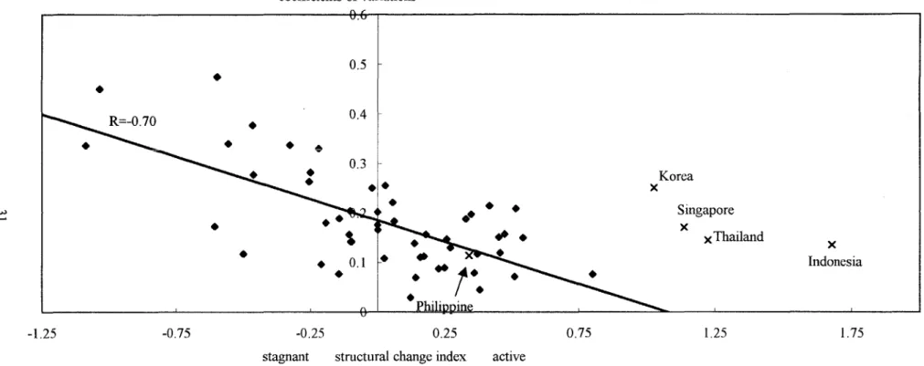
7 Movements in intersectoral terms of trade can influence industrial structures by their effects on intersectoral resource transfers. Figure 2 shows the relationship between coefficients of variations of domestic sector TOT (the ratio of agricultural and manufacturing deflators) and the extent of changes of industrial structures (the percentage decline of agriculture's share of GDP plus the percentage growth of

improvements can affect the pattern of profitability of the sector, increasing net capital inflows in the long term.

Domestic agricultural terms of trade depends on many factors, such as the international terms of trade, domestic pricing policies, and technical change in agriculture relative to non-agriculture, and so on. Specifying the factors affecting agricultural terms of trade is important because the TOT is a major factor effecting intersectoral resource transfers8.

manufacturing share of GDP, expressed as an index) of 55 developing economies in 1970-1991. This cross-section analysis clearly shows that stable TOT possibly coupled with the stabilizing effects of pricing policies can contribute to dynamic changes in the industrial structure. Actually. in the Philippines, government price interventions are motivated in part by the desire to stabilize prices.

8 David (1983) ran a regression for the domestic terms of trade of agriculture relative to

manufacturing with the following two independent variables in the case of the Philippines: (1)international terms of trade (the ratio of world agricultural prices to world manufacturing prices) and (2)the official exchange rate representing domestic economic policies (sample period was 1950-80). She found that (1)international TOT was statistically insignificant, (2)exchange rate was statistically significant and had a positive relationship with the dependent variable. The World Bank(1990) cited this finding and suggested that government pricing policies, the exchange rate in particular, was crucial in determining agricultural incentives in the Philippines. However, the same regression done by authors shows completely different results:

TOT(d) = 0.979 + 0.321TOT(i) - 0.007EXCH adj.R2=0.78 (9.71) (3.50) (-2.52)

The (d) denotes "domestic", and the data for world agricultural and manufacturing prices used to calculate international (denoted "(i)") TOT are from the HANDBOOK OF INTERNATIONAL TRADE AND DEVELOPMENT STATISTICS (UNIDO). Figures in parentheses are t-values. The sample period was 1970-1992.

Contrary to the regression by David (1983), international TOT is statistically significant and the coefficient on the exchange rate is negative. The exchange rate can work to improve or deteriorate domestic TOT depending on various conflicting factors. For example, in economies where agricultural commodities are primarily exported, and manufacturing activities are highly protected making them effectively non-tradable, devaluations in the exchange rate will benefit domestic prices of agricultural commodities over import-substituting manufacturing commodities by stimulating agricultural exports. On the other hand, domestic manufacturing prices will rise to

3. The Resource Allocation Mechanism Analyzed by Regional Data

The approach to finding intersectoral resource allocation by using regional data (the "regional" approach), as explained above, is taken in order to analyze the relationship between the intersectoral and intrasectoral capital allocation mechanisms. Intersectoral allocation is the resource allocation between the agricultural and non-agricultural sectors, and intrasectoral allocation is that between large and small farms.

According to Teranishi(1997), agricultural sectors in East Asian economies are characterized by an abundance of small farmers owning their own land, where resistance to policies unfavorable to agriculture is greater than in other economies, leading to a pro-agriculture bias against other sectors. We try to verify this political economic background in the intersectoral resource allocation analysis.

Table 4 shows some basic data for 14 geographical regions in the Philippines9. This table also shows the aggregated data for 4 kinds of regional groups which are (1) industrial regions, (2) large-farm-dominated (plantations) regions, (3) small-farm-dominated regions and (4) other agricultural regions. These are classified from their sectoral output shares and landholding siituations. Here, by analyzing the interregional resource allocation among the 4 groups, we can make some inferences about the political economy as mentioned above.

We can see that the relative per capita regional GDP of the non-agricultural regions was significantly higher than other regions (where the capital region--Metro Manila reigned). At the same time, the relative levels of per capita GDP and population shares remained almost the same from 1975 to 1994. Thus, it can be said that there is no evidence that regional economies have been converging or diverging to

each other in the long term.

some extent through the import of higher priced intermediate injputs.

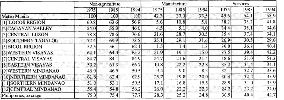
The contrast among the 4 groups in terms of sectoral output shares and landholding situations is "empirically ambiguous". Table 5 shows the sectoral distribution of output and Table 6 shows the "landholding inequality index" by regions. The "Landholding Inequality Index" is measured as the ratio of the sum of farm areas exceeding 10 hectares to total farm area.

First, Metro Manila can easily be recognized as a agricultural region since non-agricultural output accounts for 100% of its total output. However, the national average of the share of non-agricultural output to total output was also quite high at 77.7%(1994), and other regions such as Central Visayas (including Cebu province which recently has been attracting large amounts of foreign direct manufacturing investments) with 84.9% of its output non-agricultural, are not agricultural regions, either.

Second, the composition of non-agricultural output varies in each of the regions. The manufacturing sector is shown because it is the most dynamic sector of industry, and we have found that Metro Manila should not have been considered an industrial region as its share of service output is 58.9% (the share of total employment in the services industry in Metro Manila -- not presented here -- is about 70%).

Third, there are some regions which can be considered as belonging to different groups at the same time. For example, the Southern Tagalog region which includes Quezon province in its borders has large coconut plantations, and this region shows relatively large landholding inequality (Table 6). However, this region has been categorized into the non-agricultural group, rather than the large farm group which follows.

Putting aside for the time being the evaluation of the service sector in the two-sector (agriculture-industry) approach and other related problems, we dare to define the 4 groups of regions as follows,

1. Metro Manila, Central Luzon, Southem Tagalog and Central Visayas (in the central region of the Philippines) as Non-agricultural Regions

2. Bicol, Western Visayas, Western, Northern and Southern Mindanao (in the southern region of the Philippines) as Large Farm Regions

3. Ilocos and Cagayan Valley (including CAR, in the northern region of the Philippines) as Small Farm Regions

Outcomes of the findings using the regional approach follow:

[Policy-based capital outflows]

Table 7 shows the trends of policy-based net capital outflows (government revenue less government expenditure) in the above-defined 4 regional groupsl'. We can also see that the central government maintained a pro-agricultural fiscal policy as indicated by the positive sign of outflow only in industrial regions. Others show negative signs which mean there were net capital inflows into these regions from the government.

The second finding is that the relative size of capital inflows as a proportion to regional GDP" was largest in small-farm-dominated regions relative to large farm

10 Data is available for 1979 to 1993 for policy-based net capital outflows in 4 regions. Regional

tax data are collected by the Bureau of Internal Revenue (BIR). BIR collections account for

around 70% of all national government tax revenues. On the olher hand, total regional allocation of central government expenditures covers only about 30% of total central government expenditure, and the remaining 70% is used for nationwide or interregional objectives. Thus, this estimation may overestimate the net capital outflow done by the central government.

Moreover, it should be noted that the regional tax data used here does not include tariffs, export taxes,the impact of trade quotas and of other various kinds of price controls which are not necessarily tax measures, all of which are central to pricing policies and affect the domestic terms of trade of agriculture and consequently capital outflow.

" I Components of Expenditure on Gross Regional Domestic Product (1975-1993) are available from the National Statistical Coordination Board.

The Components are as follows:

1. Personal Consumption Expenditure 2. Govermuent Consumption Expenditure 3. Gross Value in Public Construction 4. Gross Value in Private Construction

5. Gross Domestic Capital Formation in Durable Equipment

6. Gross Domestic Capital Formation in Breeding Stocks and Orchard Development

7. Changes in Stocks

regions and others in almost all sample years, except 1986, 88, 90, 91. However, even in these years, the capital inflows into small farm regions were larger than into plantation regions.

These trends reflected the dramatically increasing public expenditures for agriculture allocated particularly to irrigation. Small farm regions with relatively large shares of rice production captured large amount of these expenditures. According to David(1996), irrigation was the single largest public expenditure item between 1974

and 1984. In 1984, public expenditure for irrigation was close to half of all agricultural public spending and totaled 20% of the total infrastructure budget, but dropped sharply around the mid- 1980s. These trends were reflected particularly in the relative sizes of net public capital inflows in small farm regions with relatively large shares of rice production (Table 7).

Public expenditures for agriculture in real terms increased nearly fivefold in the 1970s 2. Expressed as shares of gross value added in agriculture, and of total government expenditures, the increases were also dramatic. That rapid growth was surely motivated by high world commodity prices, and easy access to foreign development grants. However, the main motive for the increase was the serious food grain shortage in 1973. As a result, the main beneficiary of that increased

spending was the rice subsector.

This background for resource flows does not support the hypothesis presented by Teranishi(1997). The capital allocation as described above can be attributed not so much to the power of the farmers to resist policies unfavorable to agriculture as to the implementation of policies designed to mitigate the effects of the rice shortage.

[Private sector based capital outflows]

The trends in private capital allocation draw quite a different picture, as can be inferred from Table 8. Looking at the loans to deposits ratio of banks, above the even or the highest level of the ratio of non-agricultural regions indicates that private capital has been transferred from agricultural regions into non-agricultural regions. In addition, the ratio of small farm regions was lowest in almost all sample years.

It should be noted, however, that investments in bonds and securities by banks have not been added to loan portfolios due to data constraints, although these assets are

12_{David (1996) shows the central government expenditures for agriculture (1965-95) which can be}

broken down according to policy instruments, i.e.. irrigation, price stabilization, research. extention, coconut development, livestock, and others.

similar to deposits. In this case, the loan/deposit ratio will be undervalued, particularly in Metro Manila'3_.

The fact that private capital has been transferred frorn agricultural regions to non-agricultural regions is consistent with the preceding research based on national data. The real and relative levels of agricultural loans granted have declined since the latter half of the 1960s14, despite government intervention through various special agricultural credit programs. In addition, the distribution of loans have been biased in favor of larger farmers.

According to some surveys15, and even in the case of the Rural Bank which was established to extend loans mainly to small farmers, 68% of the total loans were received by high-income farmers. Moreover, because of the rapid inflation of around 20% during the 1970s, interest rates were negative in real terms. This created an excess demand for loans, which limited the flow of loans to agriculture, especially to small farmers, where costs of transactions and risks for lenders are inherently higher (David 1983).

Direct investment by establishments also shows the same tendency. Capital expenditures by manufacturing corporations concentrated on non-agricultural regions as indicated by the per capita expenditures in T'able 9.

4. The Affects of Pricing Policy on Capital Allocation

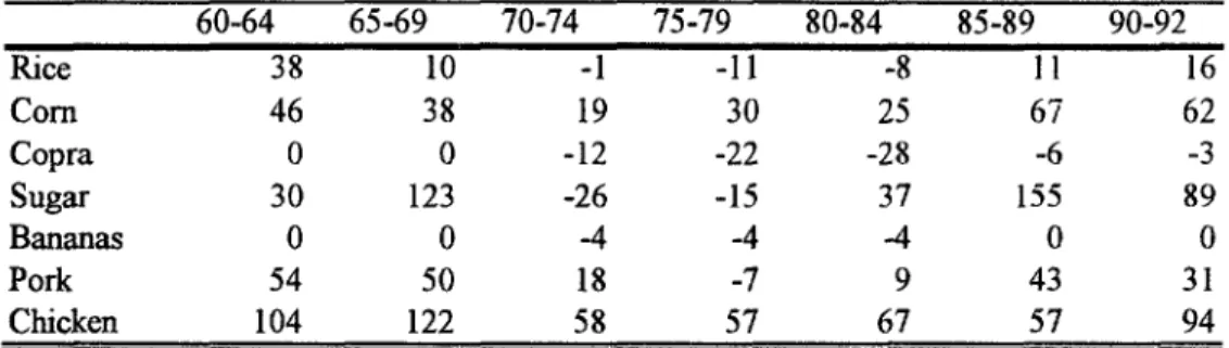
Table 10 shows the percentage difference between domestic and border prices as a measure of government price interventions into some kinds of commodity markets. Border prices are the prices without government interventions. Table 11 shows

"3The loan/deposit ratios have been under the even level in all regions after 1987 are possibly due

to some other reasons. The economic crisis of 1983-85 resulted in stricter banking regulations which have limited the lending activities of banks. For example, the reserve requirement went as high as 25% during this period and this accounts for the high 'due from Central Bank account".

On the other hand, caution should be taken in evaluating the loan/deposit ratio in the Philippines,

because growth in agricultural loans historically came mainly from the Central Bank rediscount window rather than from additional equity capital or savings deposits.

4 See David (1983), Table 9 (p45) which is based on unpublished data

estimates for the net price interventions measured as percentage differences between value added at domestic and at border prices. The latter protection rates are presented because resource allocation is affected by effective rates of protection which consider not only the policy effects on output prices, but also on intermediate input prices. Findings from these tables follow.

1. The agricultural sector has been placed under an incentive structure biased significantly in their favor compared to the manufacturing sector.

2. Price interventions have not systematically and consistently been designed to discourage all agricultural commodities in the same manner, as the nature and magnitude of the penalties imposed on each commodity were quite different from each other.

3. Protection rates generally declined over time and rose again in the late 1980s.

Point No. 2 seems to be particularly important because the political economy of the government pricing policies or "divisible benefits", the main interest of this project, will be drawn from the analysis of the protection function of different crops. In this respect, however, the World Bank (1990) pointed out that price interventions in agriculture have not been motivated by any systematic bias toward special economic interests.

The most important characteristic of Philippine politics is the "two factions and one party systemr" described as the predominance of individual loyalties over economic group interests in the political power structure, where political parties are supported by people of similar social and economic strata. Moreover, in terms of the landed aristocracy and great financial conglomerates (families), the elite class which comes from those strata had long ago branched out into industry, commerce, finance and so on. Hence, the bias of the class is not necessarily for or against agriculture or any other economic sector, for that matter. Certainly, a close link between those with political power and those with economic power is typical in the Philippines. However, we were not able to find any bias in terms of sectoral resource allocations, that has been consistently supported by these economic powers.

Campos (1991) showed empirical data to illuminate the extent that landed families controlled manufacturing activities while continuing to engage in land-based productions. He showed that: (1) among the 87 stockholding families and economic groups that control the top 120 manufacturing firms, there are 22 indigenous families (excluding foreign capital and Chinese-Filipino families) and family groups with substantial landholdings, (2) these big landed capitalist families control 33% or 40 out of the 120 leading manufacturing firms , and (3) many of

them have business partnerships with the other leading non-landed families in the top 120 manufacturing firms.

Based on the above observations, the various levels of interventions should be explained not as being socio-politically motivated as Teranishi (1997) explains. A complex set of interventions was actually intended to achieve different kinds of objectives, i.e., self-sufficiency in food supply , price-stabilization, increased government revenues, promotion of agricultural processing, balanced distribution of income and so forth.

As previously noted, the protection rates generally declined in the 1970s and rose again in the late 1980s. This suggests that government price interventions were done at least partially for price stabilization. In the first half of the 1970s, when booming world commodity prices were coupled with exchange rate devaluations, the government intervened to protect consumers from higher prices of tradable

agricultural products. The pricing policies that were biased for the consumer (pro-urban), had pro-farm (pro-rural) biases after the second half of the 1980s.

There are other factors responsible for price protection. For example, in the 1980s, the protection rates of rice did not recover to the level of the 1960s. Protection policies were in less demand as there were productivity gains in rice since the late 1960s, and this transformed the Philippines from a net importer to a net exporter of rice by the second half of the 1970s. Government investments in irrigation and extension services to disseminate a new variety of fertilizer-responsive rice were instrumental in the lowering of domestic price.

Thus, at that point, the government no longer needed to protect domestic rice production. We would like to argue that this reflects the government's apparent non-bias either for or against consumers. Maintaining low grains prices for consumers as well as assuring adequate price incentives for producers were the twin objectives of pricing policies.

5. The linkages between inter- and intra-sectoral resource allocation

mechanism

We believe one of the most important issues in resource allocation in the Philippines is the linkage between the inter- and intrasectoral resource allocation mechanism. Although this research project sheds light mainly on the contribution of intersectoral (interregional) resource allocation to economic development, we can still point out the undeniable tie between the inter- and intrasectoral(iregional) resource allocation mechanism.

In this respect, Balisacan(1994) revealed that the inter-regional component of overall inequality is rather small (no more than 20%) and the intra-regional contribution amounts to about 80% in the Philippines16_{. This outcome is quite}

contrary to the common perception that much of the inequality would be reduced by policy reforms aimed at redressing the resource allocation gap among regions and between rural and urban areas.

This finding also seems to have important implications to the regional approach in this study. That is, it becomes unclear regional grouping to represent industries is appropriate as almost all income inequality possibly coupled with unbalanced resource allocation is unexpectedly attributed to intra-regional (intra-sectoral) factor, rather than interregional (intersectoral) factor.

According to Ranis (1990), a relatively equal structure of income and asset ownership in agriculture (intrasectoral allocation) can contribute to a buoyant market for rural and labor-intensive industries (intersectoral and intraregional allocation). This leads to a spatial balance of development (interregional allocation). As these observations indicate, intra- and inter-sectoral resource allocation mechanisms are related to each other.

Regarding the intra- and inter-sectoral resource allocation mechanism, the role of huge conglomerates, constituting a very unique political and economic system in the Philippines, was discussed. No radical breach taking place between the landowning families and the manufacturing class, this capital brought a contradictory set of interests into the ISI sector, weakening the initial social coalition for industrial growth that could have directed land-based wealth into industrial capital. Because much landed capital was used for plantation agriculture for export, they opposed

16 Balisacan (1994) used the Theil index as measures of inequality. The Theil index at the

national level can be decomposed into within-group (region) contributions and between-group (region) contributions as follows, Theil: (1/n)Sln(Y/Yi) = S(nj/n)Theil (j) + S(nj/n)ln(YlYj)

=Theil (w) + Theil (b)

where Yi is the expenditure (or income) of person i n is population size

Y is the arithmetic mean expenditure (or income) j is group (region)

Theil (w) is the Theil index for within group (region) Theil (b) is the Theil index for between group (region)

exchange controls which had earlier supported the ISI. In addition, as the main opponents of land reform with redistributional effects, they failed to create a strong domestic market which would have been the basis for sustained industrial growth.

It has been pointed out that this unique system is persistent and has not changed as much as would have been expected even after the collapse of the Marcos regime. For instance, 20 years of the Marcos regime (1965-1986) saw newly developed economic powers, called "Marcos cronies", coming from a completely different background (non-landed capitals) from traditional ones (landed capitals). In the following Aquino regime, traditional landed capitals regained their power. In this course, however, their behavior -- rent-seeking -- has not changed at all. If this is correct, it is difficult to blame intersectoral resource allocation changes on changes in the political regimes.

6. Conclusion

In this chapter, we have provided an overview of the intersectoral resource allocation in the Philippines and also touched ujpon the political economic backgrounds of these flows by analyzing regional data. The most important objective of this research was to provide an analysis of the intersectoral resource flows broken down into private and public-based resource allocations.

The agricultural sector has continued to supply capital to the non-agricultural sector, and the total net transfers out of agriculture grew signiiicantly during the first half of the 1970s. The government spent more in agriculture than it gained from taxation of the sector in most years, but the magnitude of government-led inflows was too small to compensate for the capital outflows of the private sector.

Note that private based (market-based) capital allocation includes various kinds of anti-agricultural direct and indirect pricing policies (excluding tax-related policies which are included in policy-based allocations). Oftentimes, public expenditures including concessional credit programs and other types of subsidies are justified on the basis that they mitigate the penalties imposed on agriculture by other economic policies, particularly price intervention policies. In the case of the Philippines, however, the use of credit policies to compensate for the effects of policies that worsen the terms of trade against food and agricultu:ral exports will have lirnited effects.

In the findings of the regional approach taken in this project, it was interesting that the relative size of government-led capital inflows was largest in the small farm regions. As mentioned above, the relative concentration of net public capital in

small farm regions does not concur with the hypothesis presented by Teranishi(1997). This is because the capital allocation as described above can be attributed not so much to farmers' wills to resist policies detrimental to agriculture, as to the rapid growth of government expenditure for rice production after the "rice crisis" in the beginning of the 1970s. This change was not dictated by specific economic interest groups, but by political decisions driven by what the government wanted to do to achieve national goals (World Bank 1990).

We think that a further discussion should be needed in terms of the evaluation of the volume of capital allocation. The most important objective of this research was to estimate intersectoral resource allocation and then to evaluate its impact on economic development. However, we do not have a criteria to evaluate policies biased against or in favor of agricultural sector. One solution may be international comparison, but it is difficult to cover intersectoral resource flows in a same basis in other sample countries due to data constraint.

Regarding of the cause-and-effect relationship between intersectoral resource allocation and economic development, it is interesting to find a close relationship between coefficients of variations of domestic agricultural terms of trade and the extent of changes of industrial structures in 55 developing economies as shown in Figure 2. Movements in intersectoral terms of trade can influence industrial structures by their effects on intersectoral resource transfers. So, in general we would like to argue that the balanced intersectoral resource flows are closely related with the stability as well as the volume of relative resource allocation to agricultural sector.

The important issues to be discussed in resource allocation in the Philippines is the linkage between the inter- and intrasectoral resource allocation mechanism, although this research project sheds light mainly on the contribution of intersectoral (interregional) resource allocation to economic development. The interregional component of overall income inequality possibly coupled with imbalanced intersectoral resource allocation is rather small in the Philippines. The most serious problem in Philippine has been the imbalance between the rich and the poor (intrasectoral imbalance) rather than intersectoral imbalance because both agricultural and manufacturing sectors have been substantially covered by the rich landed capitals.

A transfer of capital out of agriculture will lead to sustained growth only if this is done efficiently towards more socially profitable investments coupled with a relatively balanced income distribution. In the case of Philippine, however, some great financial conglomerates are criticized for creating highly oligopolistic market structures which are seen as responsible for the inefficient resource use and uneven

income distribution. These landed capitalists have channelled massive state resources into traditional economic activities like sugar and coconut farming, limiting the country's industrial diversification.

These viewpoints seem to be justified by recent good economic performances in Philippine. Recent relatively high growth rates are achieved mainly by deregulation and relaxation of restriction President Lamos proceeds positively, which can change oligopolistic markets to more competitive resulting in per capita income growth and more inflows of foreign direct investments favoring growing domestic markets. We think a further investigation should be needed to see how the previous social and economic systems are changing and how this structural reforms influence the way of intersectoral resource allocation.

Appendix

Measuring Net Capital Outflows from Agriculture to Non-Agricultural Sector

Net capital outflows from agriculture are defined as the net real resources transferred from the agricultural to non-agricultural sectors, i.e., the difference between the food and raw materials delivered to the non-agricultural sector and the industrial consumer goods and industrial inputs flowing in the opposite direction. The agricultural sector is defined to include the production and consumption of crops, livestock and poultry, fisheries and forestry products. The non-agricultural sector consists of the rest of the economy.

(A) Accounting framework

The following is a description of the sectoral flows in agriculture.

GOODS INFLOWS

œEPENDfTRES

[Agricultural Production Sector (APS)]

Xaa+Xna+Laa+Kaa+Kna+Xma = Caa+Can+Xan+Xaa+Cae+Xae+Iaa (1)

[Agricultural household sector (AHS)]

Caa+Cna+Ta+Sa+Cma = Laa+Lan+Kaa+Kan+Ga (2)

By combining equations (1) and (2) and canceling out similar terms, the following equation (3) for agricultural sector is obtained.

(Xan+Can+Xae+Cae)-(Xna+Cna+Xma+Cma)+(Kan-Kna+Lan)

- Sa-Iaa+Ta-Ga (3)

Equation (3) states that the trade surplus in goods other than investment goods plus the trade surplus in primary inputs (land and labor; Lna is assumed to be negligible) is equal to savings minus the accumulation of stocks of agricultural products in agricultural sector plus government taxes minus expenditures. Next, to obtain the net trade surplus in agriculture, (Ina+Ima) is subtracted from both sides in equation (3) since (Ina+Ima) is the trade deficit in investment goods. Thus:

(Xan+Can+Xae+Cae)-(Xna+Cna+Xma+Cma)+(Kan-Kna+Lan)-(Ina+Ima)

- Sa-Iaa+Ta-Ga-(Ina+Ima) (4)

In equation (4), Iaa+Ina+Ima=Ia. Leon (1982) assumes there are no intersectoral transfers of production factors, i.e., Kan-Kna+Lan=0. This assumption may be due

to data constraints. Furthermore, we have to assurne Ina+Ima=O, as we cannot find appropriate allocations to disaggregate the total outputs of investment goods into agricultural and non-agricultural uses'7. Then, this equation can be rewritten as,

(Xan+Can+Xae+Cae)-(Xna+Cna+Xma+Cma) . (Sa-Ia)+(Ta-Ga) (4')

the left-hand side of the equation (4') is estimated by using Input-Output tables.

[Notations for the above equation]

X:Intermediate goods, C:Consumer goods, I:Investment (Capital goods), S:Savings, K:Capital (land), L:Labor, T:Government Tax, G:Government Services, a:Agriculture, n:Non-Agriculture, e:Exports, m:Imports, and where there are two subscripts, the order indicates the directions of the flow, i.e., Xna denotes the flow of intermediate goods from non-agriculture to agriculture.

(B)Estimation Procedures and Data Sources

Our estimation procedures are based on Leon (1982). However, Leon's approach has been slightly modified here with respect to the coverage of G. It should be noted that the left side of equation (4'), estimated by 1-0 tables, is a trade balance, not reflecting a complete IS balance of agricultural sector, since 1-0 tables do not include transfers from government to agricultural sector. The excluded transfers are, for example, government expenditures in infrastnacture, research, agricultural support services and so forth.

To extract a complete IS balance (=current account) of the agricultural sector, we have to add the transfers that have been excluded to the trade balance. Leon (1982) estimated this portion of G by adding up central and local governments' budgets which involved: 1) spending for agricultural programs/activities, i.e., expenditures of bureaus under the Ministry of Agriculture and the Ministry of Natural Resources, and 2) other spending, where there was no information on allocation, i.e., education, health, infrastructure, national defense, justice, etc., estimated by using the allocators based on agriculture's share of income, or employment, or an average of the two.

17Leon(1982) derives (Ina+Ima) by "adding up all the output of industries producing capital goods

that are used in the various agricultural subsectors. These industries include machinery,

transport equipment, and construction (p44 and Appendix F)". However, there is no information on how these outputs should be allocated..

We, on the other hand, chose to use government transfer data (T-G) from the World Bank (1990)18. This is because Leon's approach is likely to lead to inaccurate estimates of transfers from government to agriculture because it includes government's own consumption, and some statistics show that infrastructure expenditures are concentrated in industrial areas, not always proportionate to sectoral share of GDP and employment.

Intersectoral flows of C, X are calculated as follows:

(a)Can, Cna

Consumption expenditures on agricultural and non-agricultural goods (CA, CN) are broken down as CA=Caa+Cna and CN=Cnn+Cna. CA, CN can be obtained directly from the I-0 tables. To find Can and Cna, the ratios (Can/CA), and (Cna/CN) are estimated from the Family Income and Expenditure Surveys (FIES). The FIES provides percentage shares of expenditure on food and non-food items by farmer and non-farmer households in their total spending. Food and non-food correspond to agricultural and non-agricultural goods respectively. In addition, farmer and farmer households are used to represent agricultural and non-agricultural households respectively.

(b)Xan, Xna

Xan, Xna can be found in 1-0 Tables.

18 World Bank (1990), pp.25 9-262, Table 5.7. Table 5.8

Reerencs

Arsenio M. Balisacan. 1994. "Spatial Development, Land Use, and Urban-Rural Growth Linkages in the Philippines". National Economic and Development Authority.

Cristina C. David. 1983. "Economic Policies and Philippine Agriculture." Philippine Institute for Development Studies Working Paper, 83-02.

Cristina C.David. 1996. "Agricultural Policy and the WTO Agreement: The Philippine Case". Paper presented at the Conference on Food and Agricultural Policy Challenges for the Asia-Pacific, in Manila, October 1-3, 1996.

Manuel S.J. De Leon. 1982. "Intersectoral Capital Fl[ows and Price Intervention Policies in Philippine Agriculture". Unpublished Ph.D. dissertation, University of the Philippines at Los BaSfos.

Poncianao S. Intal, Jr. and John H. Power. 1990. "Trade, Exchange Rate, and Agricultural Pricing Policies in the Philippines". World Bank Comparative Studies. Anne 0. Krueger, Maurice Schiff, Alberto Valdes. 1991. "The Political Economy of Agricultural Pricing Policy". Vol 2, ASIA. The World Bank Comparative Studies.

Juro Teranishi. 1997. "Sectoral Resource Transfer, Conflict, and Macrostability in Economic Development: A Comparative Analysis". The Role of Government in East Asian Economic Development, Comparative Institutional Analysis, edited by Masahiko Aoki, Hyung-ki Kim and Masahiro Okuno-Fujiwara.

Gustav Ranis, Frances Stewart, and Edna Angeles-Reyes. 1990. "Linkages in Developing Countries: A Philippine Study". International Center for Economic

Growth.

Rivera, Temario Campos. 1991. "Class, the State and Foreign Capital: the Politics of Philippine Industrialization, 1950-1986". Ph.D. disseration, The University of Wisconsin-Madison.

Table 1 Sectoral Composition of Gross Domestic Product and Employment in Philippines (%) GDP 1955 1965 1975 1985 1990 Agriculture 33.22 30.22 26.92 28.64 26.67 Industry 25.66 28.09 33.79 32.61 33.48 Manufacturing 18.63 21.21 24.98 24.21 24.66 Services 41.12 41.69 39.29 38.75 39.85 Employment Agriculture 60.04 57.57 54.28 49.52 45.21 Industry 15.67 14.76 14.74 14.11 16.61 Manufacturing 12.37 11.31 10.97 9.59 10.21 Services 24.29 27.67 30.98 36.37 38.18

Note: Three-year averages, centered around the year shown Source: Balisacan (1993)

Table 2(a) Growth Rates of Agricultural GDP, Labor Force, P:roductivity (1977-90)

and Share in GDP (%)

Share of Agriculture in GDP (%) Average Annual Growth Rate Decline(%), Agricultural 1977 1990 1977-90 GDP Labor Productivity Philippine 26.4 23.9 9.6 1.7 2.4 -0.7 Korea 24.8 10.6 57.2 0.7 -3.8 4.5 Indonesia 27.6 21.2 23.1 3.9 2.8 1.1 China 41.9 30.4 27.4 5.1 1.4 3.6 Thailand 23.5 15.2 35.4 4.0 2.2 1.8 Malaysia 25.1 18.7 25.7 3.5 -1.0 4.4 Taipei 9.5 4.0 57.9 1.4 -3.1 4.4 Singapore 1.5 0.3 78.2 -4.3 -8.8 4.6 Bangladesh 46.3 41.3 10.7 1.8 2.9 -1.1 SriLanka 30.6 26.5 13.4 1.6 1.8 -0.2 India 40.5 31.5 22.1 2.8 0.3 2.5 Pakistan 31.6 25.5 19.4 4.5 2.2 2.3

Note: China is for 78-90, Malaysia for 78-90, Bangladesh for 77-86, Sri Lanka for 81-90

Source: Asian Development Bank, Key Indicators of Developing Asian and Pacific Countries 1995, World Bank, World Tables 1994

Table 2(b) Growth Rates of Manufactural GDP, Labor Force, Productivity (1970-90) and Share in GDP (%)

Share of Manufacture in GDP (%) Average Annual Growth Rate Growth Rate(%), Manufactural

1970 1990 1970-90 GDP Labor Productivity Philippine 25 25 0 3.5 3.1 0.4 Korea 21 31 48 13.8 6.3 7.5 Indonesia 10 20 100 12.9 6.6 6.3 Thailand 16 26 63 9.8 7.3 2.4 Malaysia 12 27 125 10.5 7.8 2.7 Singapore 20 29 45 8.9 4.3 4.6 Bangladesh 6 9 50 2.3 4.7 -2.4 India 15 18 20 5.7 2.9 2.8 Pakistan 16 17 6 6.4 1.6 4.7 Note: Shares of Manufacture in GDP of India and Pakistan are at purclhaser values.

Table 3 Net Public and Private Capital Outflows from Agriculture, 1961-1982 (% of Agricultural GVA)

Trade balance Government-led Transfers Total flows Private Public year (S-I)+T Revenue(T) Expenditure(G) (S-I)+(T-G) S-I T-G

61 6.20 1.32 2.24 3.96 4.87 -0.92 62 7.41 1.42 1.68 5.73 5.99 -0.26 63 8.76 1.66 2.91 5.85 7.10 -1.25 64 11.55 1.70 3.25 8.30 9.85 -1.55 65 12.12 1.48 2.66 9.46 10.64 -1.18 66 13.36 1.43 2.28 11.08 11.93 -0.85 67 14.27 1.34 2.07 12.20 12.93 -0.73 68 13.63 1.41 1.94 11.70 12.22 -0.52 69 13.21 1.05 2.37 10.84 12.17 -1.32 70 16.53 2.48 2.80 13.73 14.06 -0.32 71 20.91 2.83 2.59 18.32 18.08 0.24 72 25.19 2.07 3.30 21.89 23.12 -1.23 73 26.04 2.37 4.10 21.95 23.67 -1.73 74 27.84 6.18 4.57 23.27 21.66 1.61 75 27.50 4.43 4.55 22.96 23.07 -0.11 76 28.19 3.77 4.48 23.72 24.42 -0.71 77 28.76 4.46 5.09 23.67 24.30 -0.63 78 28.74 4.49 5.76 22.98 24.25 -1.27 79 29.28 3.47 5.63 23.65 25.82 -2.16 80 30.03 6.52 5.63 24.39 23.51 0.89 81 31.11 5.19 5.88 25.23 25.92 -0.69 82 30.50 2.20 5.18 25.32 28.30 -2.97 Note: Trade Balance is estimated from 1-0 tables of 1961, 65, 69, 74, 79, 83.

The estimates for in-between 1-0 years are obtained by straightline interpolation. Public transfers are from World Bank (1990)

Table 4 Regional GDP (RGDP) and Regional Population Shares in Philippine

RGDP,Per Capita (avg.=100) 1975 1980 1985 1990 1994

Philippines 100 100 100 100 100 NCR METRO MANILA 246 241 226 236 227 CAR CORDILLERA 100 105 [1]ILOCOS REGION 62 65 61 52 51 [2]CAGAYAN VALLEY 72 73 58 56 49 [3]CENTRAL LUZON 91 88 94 93 97 [4]SOUTHERN TAGALOG 118 115 111 112 119 [5]BICOL REGION 40 42 47 47 43 [6]WESTERN VISAYAS 79 79 80 79 82 [7]CENTRAL VISAYAS 76 78 81 87 89 [8]EASTERN VISAYAS 43 42 50 48 45 [9]WESTERN MINDANAO 65 60 62 56 58 [10]NORTHERN MINDANAO 102 105 97 89 88 [11]SORTHERNMINDANAO 129 114 109 95 95 [12]CENTRAL MINDANAO 78 81 83 66 71 Pop. Density Populationshare(%) 1975 1980 1985 1990 1994 of 1994 Philippines 100.0 100.0 1)0.0 100.0 100.0 223 NCRMETRO MANILA 11.8 12.3 12.7 13.1 13.1 13,799 CAR CORDILLERA 1.9 1.9 1.9 1.9 68 [1]ILOCOS REGION 6.5 6.1 7.1 5.8 5.6 294 [2]CAGAYAN VALLEY 4.0 4.0 4.6 3.9 4.0 101 [3]CENTRAL LUZON 10.0 10.0 1.0.0 10.2 10.0 368 [4]SOUTHERN TAGALOG 12.4 12.7 13.0 13.6 13.3 191 [5]BICOL REGION 7.6 7.2 7.2 6.4 7.1 271 [6]WESTERN VISAYAS 9.9 9.4 9.3 8.9 9.2 303 [7]CENTRAL VISAYAS 8.1 7.9 7.7 7.6 7.4 331 [8]EASTERN VISAYAS 6.2 5.8 5.6 5.0 5.4 168 [9]WESTERN MINDANAO 4.9 5.3 5.2 5.2 5.2 185 [10]NORTHERN MINDANAO 5.5 5.7 5.8 5.8 5.9 141 [I I]SORTHERN MINDANAO 6.5 7.0 7.0 7.3 7.1 150 [12]CENTRAL MINDANAO 4.9 4.7 4.8 5.2 4.8 139

RGDP,Per Capita (avg.=100) 1975 1980 1985 1990 1994

Philippines 100 100 100 100 100 Non-Agr.(NCR,CL,ST,CV) 139 138 136 139 141 Large(BIC,WV,WM,NM,SM) 81 80 79 75 74 Small(IL,CAG) 66 68 60 53 50 Others(EV,CM) 58 59 65 57 57 Population share (%) 1975 1980 1985 1990 1994 Philippines 100.0 100.0 100.0 100.0 100.0 Non-Agr.(NCR,CL,ST,CV) 42.3 42.9 43.3 44.5 43.8 Large(BIC,WV,WM,NM,SM) 34.3 34.6 34.6 33.7 34.5 Small(IL,CAG) 12.4 12.0 11.8 11.6 11.5 Others(EV,CM) 11.1 10.5 10.4 10.3 10.2

Table 5 Sectoral Distribution of Output by Region, 1975, 85, 94 (%)

Non-agriculture Manufacture Services

1975 1985 1994 1975 1985 1994 1975 1985 1994 Metro Manila 100 100 100 42.3 37.0 33.5 45.6 54.1 58.9 [I]ILOCOS REGION 60.8 63.6 56.9 5.6 10.8 5.8 38.2 35.2 41.8 [21CAGAYAN VALLEY 54,0 55,3 46.0 4.5 5.1 4.0 34.4 35,1 34.6 [3]CENTRAL LUZON 78.8 78.6 76.6 31.6 28.7 30.5 35.4 37.4 34.1 [4]SOUTHERN TAGALOG 72.4 69.9 73.5 35.1 29.1 31.6 26.9 30.5 29.6 [5]BICOL REGION 52.5 56.1 62.1 1.5 1.4 1.3 39.0 36.8 40.4 [6]WESTERN VISAYAS 64.1 64.4 65.2 21,9 19.1 15.0 37.5 39.4 42.2 [7]CENTRAL VISAYAS 84.7 84.1 84.9 24.7 21.6 21.4 48.6 51.0 54.3 [8]EASTERN VISAYAS 59.2 61.9 66.7 10.8 22.2 22.8 35.3 31.4 34.1 [9]WESTERN MINDANAO 46.9 46.5 50.5 9.4 9.0 8.3 32.1 32.7 33.6 [IOJNORTHERN MINDANAO 61.8 62,4 62.9 25.7 19.8 20.0 30.4 32.2 35.9 [ 1]SORTHERN MINDANAO 51.0 53.1 59.5 17.1 16.8 15.5 28.9 31.0 35.9 [121CENTRAL MINDANAO 55.4 54.81 56.2 26.0 22.2 22.3 24.2 23.2 24.0 Philippines, average 75.3 75.4 77.7 28.3 25.2 24.8 36.9 40.4 42.7

Table 6 Landholding Inequality Index (%) 1980 1990 Philippines, average 26 24 [1]ILOCOS REGION 12 6 [2]CAGAYAN VALLEY 23 13 [3]CENTRAL LUZON 9 12 [4]SOUTHERN TAGALOG 28 25 [5]BICOL REGION 35 28 [6]WESTERN VISAYAS 38 33 [7]CENTRAL VISAYAS22- 1 [8]EASTERN VISAYAS 23 20 [9]WESTERN MINDANAO 25 26 [1O]NORTHERN MINDANAO 28 26 [11]SORTHERNMINDANAO 32 29 [12]CENTRAL MINDANAO f106 21

Note: Landholding inequality is expressed as the ratio of the sum of farm area of farms larger than 10 hectares to the total farm area in the region. Shadowed boxes are under the national average Source: Census of Agriculture

Table 7 Central Government Revenue from minus Expenditure to Regions (% of Regional GDP) Regional Gruops 1979 1980 1981 1982 1983 1984 1985 1986 1987 1988 1989 1990 1991 1992 1993 Non-Agri(NCR,CL,ST,CV) 4.5 4.6 4.4 2.1 3.3 4.0 5.0 4.6 5.6 5.8 6.3 7.8 7.5 8.4 Large(BIC,WV,WM,NM,SM) -2.9 -4.0 -3.4 -4.8 4.0 -2.7 -2.4 -2.8 -4.3 51 -5.0 -3.4 -4.0 -4.3 Small(IL,CAG) -83 -10.3 -9.5 -115 -10.7 71 -5.8 -6.4 -9.2 -10.9 -11.1 -79 -9.5 -9.7 Others(EV,CM) -7.3 -8.9 -8.7 -10.9 -8.6 -. 5 -5.7 -. 9 -9.7 -10.7 -11.9 -8.4 -9.3 -9.2

Note: Data for 1987 is not available Minus means inflows to regions

Source: Annual Financial Report of the National Government, Annual Report of Bureau of Internal Revenue, various years

Table 8 Loan Portfolio to Deposit Ratio of Banking Oflious

Regional Gruops 1977 1978 1979 1980 1981 1982 1983 1984 1985 1986 1987 1988 1989 1990 1991 19921 1993 1994 Non-Agri(NCR,CL,ST,CV) 1.46 1.48 1.43 1.33 1.44 1.31 1.52 1.45 1.13 1.13 0.74 0.77 0.77 0.84 0.82 0.80 0.87 0.89 Large(BIC,WV,WM,NM,SM) 1.50 1.35 1.42 1.52 1.59 1.46 1.39 1.08 1.00 0.84 0.66 0.63 0.60 0.57 0.53 0.60 0.65 0.68

t) Small(IL,CAG) 1.21 1.09 1.04 1.05 1.02 0.98 0.91 0.75 0.63 0.54 0.45 0.38 0.40 0.37 0.36 0.36 0.52 0.59 Others(EV,CM) 1.16 1.18 1.23 1.40 1.37 1.23 1.22 0.96 0.83 0.57 0.43 0.41 0.32 0.33 0.37 0.41 0.46 0.52

Table 9 Numbers of Establishments and Capital Expenditures in Manufactures

(1) Numbers of Establishments Per Capita

Region 1960 1970 1985 1990* 1975** 1980**

PHULIPPINES, Average 0.070 0.059 0.050 0.172 1.830 1.774

Non-Agri. (NCR, CL, ST, CV) 0.143 0.113 0.077 0.305 2.093 1.991

Large (BIC, WV, WM, NM, SM) 0.023 0.021 0.035 0.075 1.591 1.502

Small (IL, CAG) 0.009 0.010 0.012 0.063 2.275 2.439

Others (EV,CM) 0.035 0.032 0.019 0.041 1.071 1.023

(2) Capital Expenditures Per Capita (Pesos)

Region 1960 1970 1975 1985 1990* 1980**

PHILIPPINES, Average 9.1 35.7 81.5 128.5 494.6 157.2

,s Non-Agri. (NCR, CL, ST, CV) 18.9 53.1 152.1 219.6 893.3 270.5

Large(BIC,WV,WM,NM,SM) 3.0 37.1 38.3 28.4 173.7 118.9

Small (IL, CAG) 1.1 1.4 8.0 30.5 100.5 44.0

Others (EV,CM) 4.2 7.9 27.4 192.5 267.2 131.4

Note: (*) is for establishments with employment of 10 or more, (**) is for all size. Others are for only large farms

Table 10 Nominal Protection Rates of Selected Agricultural Commodities, 1960-92 60-64 65-69 70-74 75-79 80-84 85-89 90-92 Rice 38 10 -I -11 -8 11 16 Corn 46 38 19 30 25 67 62 Copra 0 0 -12 -22 -28 -6 -3 Sugar 30 123 -26 -15 37 155 89 Bananas 0 0 -4 -4 -4 0 0 Pork 54 50 18 -7 9 43 31 Chicken 104 122 58 57 67 57 94 Source: David (1996)

Table 11 Estimated Effective Protection Rates

Agri. Manu. All

1974 9.0 44.0 36.0 1983 10.3 79.2 52.8 1985 9.2 74.1 49.3 1986 5.0 61.2 39.8 1988 5.2 55.5 36.3 Source: David (1996) 29

Figure 1 Domestic terms of trade of Philippine (1960-94) Index(1988=100) 130 120 110 100 90 80 60 62 64 66 68 70 72 74 76 78 80 82 84 86 88 90 92 94 year Terms of trade: agricultural deflator / manufacturing deflator

Figure 2 The Relationship Between Coefficients of Variations of Domestic Agricultural Terms of Trade and Changes in Industrial Structures for 55 developing economies (1970-91) coefficients of variations 0.6 0.5 0.4 Korea x Singapore S + ~ xThailand x 0|1 * O I PhilippinIndonesia -1.25 -0.75 -0.25 0.25 0.75 1.25 1.75 stagnant structural change index active

Note: Structural change index is calculated as the percentage decline of the share of agriculture in GDP plus the percentage growth of the share of manufacturing in GDP in 1970-91. Terms of trade is the agricultural deflator/manufacturing deflator. R=-0.70 refers to data excluding the four East Asian economies on the far right.

Policy Research Working Paper Series

Contact

Author Date for paper

'VP S185 S1&35 iv.irqr %uo,ess: Policy Reform Susmita Dasgupta November 1997 S. Dasgupta

an,, thie s_h,Fe o' Industrial Hua Wang 32679

Foi otio, i <.,naDavid Wheeler

WAFS18 57 Leasing tc Supoort Small Businesses Joselito Gallardo December 1997 R. Garner

and Mic,oenerprises 37664

VP S It58 52nking on the Poor) Branch Martin Ravallion December 1997 P. Sader lacerent arnd Nonfarm Rural Quentin Wodon 33902 Development in Bangladesn

VP S I 9 L eEsors froam SSo Paulo's Jorge Rebelo December 1997 A. Turner

Mielv-opoitan Busway Concessions Pedro Benvenuto 30933

Progra,n

.VPS I S0 ihe Heatyn Effects of Air Poliution Maureen L. Cropper December 1997 A. Maranon

Nathalie B. Simon 39374

Anna Alberini P. K. Sharma

VWJPSiS61 nfnastru-tuLre Project Finance and Mansoor Dailami December 1997 M. Dailami Capital Flows: A New Perspective Danny Leipziger 32130 WPS-i8,52 Spatial Poverty Traps? Jyotsna Jalan December 1997 P. Sader

Martin Ravallion 33902

WPS1 I 863 .Are the Poor Less Well-nsured? Jyotsna Jalan December 1997 P. Sader Evidence on Vulnerability to Income Martin Ravallion 33902 Risk in Rure, China

VVPS1 84 Child Mcrtaitih and Public Spending Deon Filmer December 1997 S. Fallon or Health: How Much Does Money Lant Pritchett 38009 Mattr?

,I,PS ,8.35 Pens,o,p Reforrn in Latin America: Sri-Ram Aiyer December 1997 P. Lee

0.I F.xe,-!as or Sustainable Reform? 37805

WVPSi855 Circun nstnce anid Choice: The Role Martha de Melo December 1997 C. Bernardo

,i 2, Condjtions and Policies in Cevdet Denizer 31148

Transi,ion Econcmiss Alan Geib

Stoyan Tenev

WiPS l 8i5-F7 Gander lispmrity in South Asia: Deon Filmer January 1998 S. Fallon Compsr,sons Setfveen and Within Elizabeth M. King 38009 C fj un-iZ F es S Lant Pritchett

VPS S8It8 oGovernment Support to Private Mansoor Dailami January 1998 M. Dailami

inrrestruoc:.re Dproiects in Emerging Michael Klein 32130 ,Mare'.sC

Policy Research Workini; Paper Series

Contact

Titlq Author Date for paper

WPS1 869 Risk Reducation and Public Spending Shantayanan Devarajan January 1998 C. Bernardo

Jeffrey S. Hammer 31148

WPSI 870 The Evolution of Poverty and Raji Jayaraman January 1998 P. Lanjouw

Inequality in Indian Villages Peter Lanjouw 34529

WPS1871 Just How Big Is Global Production Alexander J. Yeats January 1998 L. Tabada

Sharing? 36896

WPS1872 How Integration into the Central Ferdinand Bakoup January 1998 L. Tabada

African Economic and Monetary David Tarr 36896

Community Affects Cameroon's Economy: General Equilibrium Estimates

WPS1873 Wage Misalignment in CFA Countries: Martin Rama January 1998 S. Fallon

Are Labor Market Policies to Blame? 38009

WPSI 874 Health Policy in Poor Countries: Deon Filmer January 1998 S. Fallon

Weak Links in the Chain Jeffrey Hammer 38009

Lant Pritchett

WP51875 How Deposit Insurance Affects Robert Cull January 1998 P. Sintim-Aboagye

Financial Depth (A Cross-Country 37644

Analysis)

WPS1876 Industrial Pollution in Economic Hemamala Hettige January 1998 D. Wheeler

Development (Kuznets Revisited) Muthukumara Mani 33401

David Wheeler

WPS1877 What Improves Environmental Susmita Dasgupta January 1998 D. Wheeler

Performance? Evidence from Hemamala Hettige 33401

Mexican Industry David Wheeler

WPS1878 Searching for Sustainable R. Marisol Ravicz February 1998 M. Ravicz

Microfinance: A Review of Five 85582

Indonesian Initiatives

WPS1879 Relative prices and Inflation in Przemyslaw Wozniak February 1998 L. Barbone

Poland, 1989-97: The Special Role 32556

of Administered Price Increases

WPS1880 Foreign Aid and Rent-Seeking Jakob Svensson February 1998 R. Martin

39065

WPS1881 The Asian Miracle and Modern Richard R. Nelson February 1998 S. Jonnakuty

Growth Theory Howard Pack 37902

WPS1882 Interretional Resource Transfer and Toshihiko Kawagoe February 1998 R. Martin