Heat transfer enhancement of vapor condensation heat exchanger

Heat Transfer Enhancement of Vapor Condensation Heat Exchanger

________________________________________

A Dissertation

Presented to the

Faculty of the Graduate School

at the University of Missouri-Columbia

________________________________________

In Partial Fulfillment

of the Requirements for the Degree

Doctor of Philosophy

________________________________________

by

Husam Rajab

Dr. Hongbin Ma, Dissertation Supervisor

May 2017

The undersigned, appointed by the dean of the Graduate School, have examined the dissertation entitled

Heat Transfer Enhancement of Vapor Condensation Heat Exchanger presented by Husam Rajab,

a candidate for the degree of Doctor of Philosophy in Mechanical Engineering, and hereby certify that, in their opinion, it is worthy of acceptance:

_____________________________________________

Professor Hongbin Ma

_____________________________________________

Professor Gary Solbrekken

_____________________________________________

Professor Yuwen Zhang

_____________________________________________

Professor Matt Maschmann

_____________________________________________

Professor Shubhra Gangopadhyay

ii

ACKNOWLEGEMENT

I would like to thank my Ph.D supervisor Dr. Hongbin Ma for his patient guidance and solid support of my research project and my degree program. Without his academic insight and encouragement, this dissertation would not have been possible. I would like to thank my dissertation committee Dr. Gary Solbrekken, Dr. Yuwen Zhang, Dr. Matt Maschmann and Dr. Shubhra Gangopadhyay for their time and efforts. Their broad knowledge and many stimulating discussions are invaluable and greatly appreciated. I would also like to thank all the students, professors and staff of Mechanical and Aerospace Engineering department for their support and help driving me to complete my Ph.D degree successfully.

Finally I would like to thank my family and my friends for their continuous support and encouragement to complete my research and final dissertation.

The supports of the MU Innovations Fund (IF) Center and the MU College of Engineering CNC Milling Machine Laboratory are gratefully acknowledged.

iii

TABLE OF CONTENTS

ACKNOWLEDGEMENT ... ii

LIST OF FIGURES ... v

LIST OF TABLES ... viii

LIST OF SYMBLES ... ix

ABSTRACT ... xii

CHAPETER 1: INTRODUCTION ... 1

1.1. PRINCIPLES OF CONDENSATON AND EVAPORATION ... 1

1.2. COOLING TOWER MATERIALS SELECTION ... 2

1.3. IDENTIFYING STEAM POWER SYSTEMS ... 3

1.4. OBJECTIVE & RESEARCH APPROACH ... 4

CHAPETER 2: HEAT TRANSFER ENHANCEMENT USING MINI/MICRO ELLIPTICAL PIN-FIN HEAT SINKS WITH NANOFLUIDS ... 6

2.1. INTRODUCTION ... 6

2.2. MATHEMATICAL MODEL AND GOVERNING EQUATIONS... 7

2.3. SOLUTION AND PREDICTION PROCEDURE ... 12

2.4. GRID INDEPENDENCY AND CODE VALIDATION ... 13

2.5. EXPERIMENTAL DESIGN ... 15

2.6. RESULTS AND DISCUSSION ... 23

2.7. SUMMARY ... 31

CHAPTER 3:UTILIZATION OF THIN FILM EVAPORATION IN A TWO-PHASE FLOW HEAT EXCHANGER ... 38

3.1. INTRODUCTION ... 38

iv

3.3. RESULTS AND DISCUSSION ... 47

3.4. SUMMARY ... 55

CHAPTER 4: NON-DIMENSIONAL ANALYSIS OF TWO-PHASE FLOW AND CONDENSATION HEAT TRANSFER IN POROUS MEDIUM ... 56

4.1. INTRODUCTION ... 56

4.2. ANALYSIS ... 56

4.2.1. THEORETICAL MODEL ... 56

4.2.2. SOLUTION AND PREDICTION PROCEDURE ... 72

4.3. RESULTS AND DISCUSSION ... 72

4.4. SUMMARY ... 77

CHAPTER 5: VAPOR CONDENSATION HEAT TRANSFER IN POROUS MEDUM ... 78

5.1. INTRODUCTION ... 78

5.2. GOVERNING EQUATIONS ... 81

5.3. RESULTS AND DISCUSSION ... 89

5.4. SUMMARY ... 96

6. CONCLUSIONS ... 97

APPENDICIES ... 100

APPENDIX A: POROUS MEDIUM MATHEMATICAL DERIVATIONS ... 99

APPENDIX B: DESIGN AND MANUFACTURING OF MPFHS ... 105

APPENDIX C: C1. HEAT SINK PROGRAMMING CODES ... 106

APPENDIX C: C2. POROUS MEDIUM PROGRAMMING CODES ... 107

APPENDIX C: C3. HEAT SINK EXPERIMENTAL DESIGN CALCULATIONS .... 117

REFERENCES ... 127

v

LIST OA FIGURES

FIG.1.1. VAPOR-TO-CONDENSATE HEAT EXCHANGER PROCESS... 1

FIG.1.2. DIRECT & INDIRECT COOLING SYSTEM ... 3

FIG.1.3. WATER FLOW IN ONCE-THROUGH COOLING ... 4

FIG.1.4. TYPICAL VAPOR CONDENSATION SYSTEM ... 5

FIG.2.1. SCHEMATIC OF THE ELLIPTICAL PIN-FIN HEAT SINK. (LEFT: PINS ARRANGED AT THE SAME ANGLE; RIGHT: PINS ARRANGED AT DIFFERENT ANGLES; 0,22.5,45,67.5, AND 90) ... 8

FIG.2.2.(a) COMPUTATIONAL DOMAIN ... 10

FIG.2.2.(b) NONUNIFORM COMPUTATIONAL GRID: (TOP): PINS HAVE SAME ORIENTATION ANGLES, AND (BOTTOM): PINS HAVE DIFFERENT ORIENTATION ANGLES. ... 14

FIG.2.3. SCHEMATIC OF EXPERIMENTAL SETUP ... 15

FIG.2.4. PRODUCTION OF MPFHS, PROTOTYPE (I) ... 16

FIG.2.5. PRODUCTION OF MPFHS, PROTOTYPE (II) ... 19

FIG.2.6. SCHEMATIC OF TEST SECTION ... 20

FIG.2.7.(a) VISUALIZATION OF THE FLOW PATTERN: TOP: CURRENT RESULTS, BOTTOM: RESULTS OF OHMI ET AL [34]... 21

FIG.2.7.(b) A PHOTOGRAPH OF THE EXPERIMENT... 22

FIG.2.8. FLUID AND SURFACE AXIAL TEMPERATURE VARIATIONS ... 22

FIG.2.9. HEAT TRANSFER COEFFICIENT ALONG THE LENGTH OF THE PIN FIN HEAT SINK ... 23

FIG.2.10. TEMPERATURE & VELOCITY DISTRIBUTIONS AROUND TWO DIFFERENT CONFIGURATIONS OF ELLIPTICAL PIN FINS AT THREE DIFFERENT REYNOLDS NUMBERS WITH NANOFLUID AS COOLANT. ... 31 FIG.2.11.(a-f). EFFECT OF PIN ORIENTATION AND NANOFLUID VOLUME FRACTION ON NUSSELT NUMBER AT VARIOUS REYNOLDS NUMBERS, (a) NUSSELT NUMBER

vi

OF FIRST PIN, (b) NUSSELT NUMBER OF SECOND PIN, (c) NUSSELT NUMBER OF THIRD PIN, (d) NUSSELT NUMBER OF FORTH PIN, (e) NUSSELT NUMBER OF FIFTH PIN, (ef) OVERALL NUSSELT NUMBER OF HEAT SINKOF PIN ORIENTATION AND NANOFLUID VOLUME FRACTION ON NUSSELT NUMBER AT VARIOUS REYNOLDS

NUMBERS ... 35

FIG.2.12. EFFECT OF PIN ORIENTATION AND NANOFLUID VOLUME FRACTION ON EULER NUMBER... 37

FIG.3.1. SCHEMATIC OF THIN FILM EVAPORATION ... 39

FIG.3.2. DIMENSIONLESS MICROLAYER PROFILE & FILM THICKNESS AT VARIOUS SUPERHEATS ... 49

FIG.3.3. DIMENSIONLESS MICROLAYER PROFILE & HEAT FLUX AT VARIOUS SUPERHEATS ... 49

FIG.3.4. TEMPERATURE PROFILES AND PATHS FOR EVAPORATION ... 51

FIG.3.5. SUPERHEAT EFFECTS ON THIN FILM PROFILES ... 52

FIG.3.6. DIMENSIONLESS FILM THICKNESS, LIQUID, VAPOR, CAPILLARY AND DISJOINING PRESSURES ... 53

FIG.3.7. LIQUID PRESSURE DIFFERENCE AT VARIOUS SUPERHEATS ... 54

FIG.3.8. INTERFACE TEMPERATURE OF THE THIN FILM AT VARIOUS SUPERHEATS ... 54

FIG.3.9. CURVATURE PROFILES AT VARIOUS SUPERHEATS ... 55

FIG.4.1. VAPOR CONDENSATION HEAT EXCHANGER ... 56

FIG.4.2. VARIATIONS OF

u

*_F WITH DIMENSIONLESS FRONT LOCATION ... 73

FIG.4.3. VARIATIONS OF

u

*_F WITH DIMENSIONLESS LOCATION ... 73

FIG.4.4. VARIATIONS OF



F* WITH DIMENSIONLESS LOCATION ... 74

vii

FIG.4.6. VARIATIONS OF

p

_v* WITH DIMENSIONLESS LOCATION ... 75

FIG.4.7. VARIATIONS OF

p

_v* WITH DIMENSIONLESS FRONT LOCATION ... 75

FIG.4.8. VARIATIONS OF



_T WITH DIMENSIONLESS FRONT LOCATION ... 76

FIG.4.9. PROILES FOR FLUID TEMPERATURE, PRESSURE, SATURATION, AND THE VELOCITY OF THE VAPOR PHASE ... 77

FIG.5.1. CONDENSATION FLOW LENGTH IN TERMS OF TIME ... 93

FIG.B.1. SCHEMATIC OF CNC MACHINING ... 105

FIG.B.2. PHOTOGRAPH OF PROTOTYPE I ... 106

FIG.C.1. PHOTOGRAPH OF EXPERIMENTAL PROTOTYPE ... 107

FIG.C.2. PHOTOGRAPH OF CNC MACHINE PROTOTYPE... 110

FIG.C.3. CONTOUR OF VELOCITY DISTRIBUTION ... 114

FIG.C.4. FOUR BOLTS TO TIGHTEN LEXAN SHEETS ... 117

viii

LIST OA TABLES

TABLE 2.1. EXPERIMENTAL DESGIN CACULATIONS ... 20 TABLE 2.2. COMPARISON BETWEEN DATA OF KOSAR AND PELES [33] AND

CURRENT DATA ... 35 TABLE 2.3. COMPARISON BETWEEN RESULTS OF YANG ET AL [32] AND CURRENT RESULTS ... 36 TABLE 3.1. PROPERTIES OF THE WORKING FLUID FC-72 ... 47 TABLE 3.2. DIMENSIONAL PARAMETERS & CALCULATED VALUES ... 49 TABLE 3.3. COMPARISON OF THE CALCULATED RESULTS WITH PREVIOUS

MODELS ... 55 TABLE 5.1. PROPERTIES OF DIFFERENT POROUS MEDIUMS AND TWO WORKING FLUIDS... 96

ix

LIST OF SYMBLES

A = cross-sectional area, projected area of meniscus,m2 Bo = Bond number

p

c = specific heat capacity, 1 1

J kg K  Ca = capillary number E C = Ergun coefficient p d = particle diameter,

m

D = total axial diffusivity, 2 1

m s f = force, N

 

f Z = function of Z g = gravitational constant, _ms2 lv i  = heat of vaporization, _{J kg}1 Ja = Jakob number K = absolute permeability, 2 m k = conductivity, _{W m K}1 1 e k = effective conductivity, 1 1 W m K  r K = relative permeability * K = reduced permeability

n = volumetric rate of production, 1

s

p = pressure, Pa

c

p = capillary pressure, Pa

l

Pe = liquid Peclet number R = radius of glass particle Re = Reynolds number

s

= liquid saturation

t = time,

s

x u = superficial velocity, 1

m s

F

u = condensation forepart velocity

x

= axial location,

m

p

r = pore radius,

m

eff

r = effective pore radius,

m

R = radius of sphere at the contact line,

m

Re = Reynolds number, eff h

eff uD  

s

= saturation t = time,

s

T = temperature, K u = pore velocity,

m s

D u = Darcy velocity, u_D u ,

m s

V = volume, 3 m z = length

Z = length of region, coordinate

 = difference Greek symbols

l

 = liquid diffusivity, m s2 1

l

 = thickness of liquid region,

m

lv

 = thickness of two phase region,

m



= porosity  = viscosity, 1 1 s kg m   = density, 3 kg m



= surface tension, 1 N m Subscripts

eff

= effective e = exit

xi F = forepart g = gas i = initial l = liquid m = modified

s

= solid

sat = thermodynamic saturation state

tr = transition 0 = inlet 1 = first 2 = second Superscript * = dimensionless

xii

HEAT TRANSFER ENHANCEMENT OF VAPOR CONDENSATION HEAT EXCHANGER

Husam H. Rajab

Dr. Hongbin Ma, Dissertation Supervisor ABSTRACT

A typical vapor condensation condenser consists of two major heat transfer processes, i.e., vapor condensation and forced convection. In order to enhance heat transfer, the condensation heat transfer utilizing the porous medium is investigated, and at the same time, the elliptical pin fin effect on the forced convection of nanofluid studied. The forced convective heat transfer on nanofluids in an elliptical pin-fin heat sink of two different pin orientations is numerically studied by using a finite volume method.

With increasing Reynolds number, the recirculation zones behind the pins increased. There were more recirculation zones for the pins with different angular orientations than for pins with the same angular orientation. It is observed that the Nusselt number for the pins with different angular orientations was higher than that for pins with the same angular orientation. The results show that with increasing volume fraction of nanoparticles and angular orientation of pins for a given Reynolds number, Euler and Nusselt numbers as well as overall heat transfer efficiency increase.

The non dimensional mass, momentum and energy equations based on non dimensional pressure, temperature, heat capacity, capillary, and bond numbers are developed for the vapor condensation occurring in the porous medium. The volumetric viscous force for the flow is described by Darcy’s law. For the microscopic interfacial shear stress, a permeability term that relates flow rate and fluid physical properties (i.e. viscosity) to pressure gradient

xiii

l

l l l

K  u  p is implemented. The effects of permeability, porosity, and effective pore radius parameters on porous medium performance are introduced.

The occurrence of thin liquid film inside pores is addressed and the Laplace-Young equation is depicted. In calculations the Darcy-Ergun momentum relation is implemented which provide accurate means to determine the capillary performance parameters of porous medium. The dimensionless thicknesses of the two-phase and liquid regions and embodiment of unique characteristics based on the total thermal diffusivity and absolute permeability are depicted. Therefore, analyses of the phase change and two-phase flow are made by defining regions, over which appropriate approximations are made.

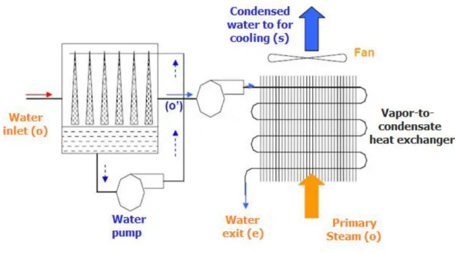
1 CHAPTER ONE: INTRODUCTION

1.1PRINCIPLES OF CONDENSATION AND EVAPORATION

As shown in figure 1.1, in a vapor-to-condensate heat exchanger process, two streams of water- primary and steam-secondary are used. The primary cold water becomes hot by coming in direct contact with the heated from bottom surface (o-o’), while the secondary steam which is used as supply condensed water to the cooling tower, decreases its temperature by exchanging only sensible heat with the cooled and water stream (o-s). Thus vapor content of the supply steam remains constant in an indirect cooling system (Figure 1.2), while its temperature drops. Obviously, everything else remaining constant, the temperature drop obtained in a direct cooling system is larger compared to that obtained in an indirect system, in addition the direct cooling system is also simpler and hence, relatively inexpensive.

2

However, since the steam content remains constant in an indirect process, this may provide greater degree of comfort in regions with higher vapor-to-condensate ratio. In modern day indirect coolers, the conditioned steam flows through tubes or plates made of non-corroding plastic materials such as polystyrene (PS) or polyvinyl chloride (PVC). On the outside of the plastic tubes or plates thin film of water is maintained. Water from the liquid film on the outside of the tubes or plates evaporates and cools through the tubes or plates sensibly. Even though the plastic materials used in these coolers have low thermal conductivity, the high external heat transfer coefficient due to evaporation of water makes up for this. The commercially available indirect coolers have saturation efficiency as high as 80%.

1.2COOLING TOWER MATERIALS SELECTION

If pre-cooling the dry steam is the objective then a wet media pad should be used to cool the dry steam before it reaches the condenser coils. In this case the type of media used is of greatest importance. The important characteristics when choosing a material are the pressure drop through it, how well it condenses the steam or cooling efficiency, and how it holds up to water damage. Water damage will deteriorate the material’s performance because of salts deposits and mold formation. This will lower the cooling efficiency and increase the pressure drop. Another consideration that should not be neglected when selecting the material is the cost. This is very important when analyzing a system’s economic advantage.

3

Fig 1.2. Direct & Indirect Cooling System 1.3IDENTIFYING STEAM POWER SYSTEMS

Currently nine out of ten power plants in the United States that generate electricity from steam power (Fig. 1.3) require condensate cooling. These systems are categorized as either once-through or wet-recirculation. Once-once-through cooling systems discharge water directly after it has absorbed system heat. Wet-recirculating systems (wet-cooling) operate in a closed loop where a considerable amount of water is lost in the cooling towers through evaporation cooling. The remaining power plants use air for heat removal in a process called dry-cooling. This process reduces water consumption by more than 90%.

However, air as a lower heat capacity than water making this design less efficient resulting in significant increases in size and cost. In summer, when electricity demand peaks, ambient temperature increases, this significantly decreases the temperature difference between steam and ambient air resulting in a decrease of cooling capacity. In order to significantly reduce or eliminate the use of water for cooling power plants, a highly efficient heat exchanger for the vapor condensation is needed.

4

Figure 1.3. Water flow in once-through cooling

1.4OBJECTIVES & RESEARCH APPROACH

For a typical vapor condensation heat exchanger, as shown in Fig. 1.4, the steam from the power plant is condensed inside the heat exchanger. The heat released from the condensation is transferred through the exchanger wall and removed by the forced convection. In order to enhance heat transfer of the condensation heat exchanger, the condensation heat transfer occurring inside the heat exchanger is needed to be increased and the forced convection heat transfer is needed to be enhanced as well. In the current investigation, the heat transfer enhancement of forced convection using elliptical pin fins is investigated. At the same time, the vapor condensation occurring in the porous medium addressed.

5

Figure 1.4. Typical Vapor Condensation System

In order to increase the heat transfer rate of the vapor condensation heat exchanger, the current investigation will focus on the condensation heat transfer and forced convection. For the vapor condensation, in order to increase the condensation heat transfer rate, porous medium is utilized to increase the condensation area, and at the same time, the condensate can be effectively removed by the capillary force. The heat released from the condensation must be efficiently removed for the forced convection. In order to increase the heat transfer coefficient of forced convection, the elliptical pin fins with nanofluid is investigated.

6

CHAPTER TWO: HEATTRANSFER ENHANCEMENT USING MINI/MICRO ELLIPTICAL PIN-FIN HEAT SINKS WITH NANOFLUIDS

2.1. INTRODUCTION

In recent years, nanofluids (NFs) have proven to have a great potential for enhancing the heat transport capability of heat transfer devices [1-8]. Therefore, using nanofluids as a working fluid is well suited for use in high performance compact heat exchangers and heat sinks used in electronic equipment. One of the important characteristics of nanofluids is represented by their higher thermal conductivities with respect to conventional coolants. The enhancement of thermal conductivity of NFs depends on particle diameter and volume fraction, thermal conductivities of base fluid and nanoparticles as well as Brownian motion of nanoparticles, which is a key mechanism in thermal conductivity enhancement. Several correlations have been developed regarding the thermal conductivity of copper oxide and water nanofluids [9-18]. Wang and Mujumdar [9] gave a quality review of such correlations. The Hamilton-Crosser (HC) model [10] and Maxwell model [11] include the effects of distribution and the interfacial layer at the particle/liquid interface along with the Brownian motion of nanoparticles, which are some key mechanisms of thermal conductivity enhancement. Koo and Kleinstreuer [12] proposed a thermal conductivity model that takes into account the effect of temperature, particle volumetric concentration, and properties of base fluid as well as nanoparticles subjected to Brownian motion. Comparisons between models [13, 14] show that Koo and Kleinstreuer’s model better captured the results of an experimental study by Namburu et al. [15], and it predicted thermal conductivity of nanofluids better than other available models [16-18].

Many experimental and numerical studies in the literature focus on heat transfer enhancement of pin shapes and their angular orientation in pin-fin heat sinks and pin fin arrays

7

[19-21]. Sparrow and Vemuri [19] have shown that fin array and its orientation have a positive influence in heat transfer. Rubio-Jimenez et al. [20] analyzed the effect of shape of pin on temperature distribution and pressure drop in micro pin-fin heat sinks. The results showed that the fin shape plays an important role in the pressure drop rather than heat dissipation. They showed that the best performance can be obtained with flat-shaped fins. Huang and Sheu [21] studied fluid flow in micro heat sink so as to obtain temperature field and distribution of Nusselt number on the square micro-pin-fin heat sink for the steady incompressible flow of Newtonian fluids. They found that the averaged value of Nusselt number increases with increasing Prandtl and Reynolds numbers.

Investigations into the optimization of geometrical structures of micro/mini heat sinks, and the use of nanofluids in cooling devices for cooling electronic equipment are still embryonic; much more study is required in order to better understand the thermal and fluid dynamic characteristics of these devices with this very promising new family of coolants and different geometries. Therefore, in the current investigation, an analysis was conducted to determine the effect of nanofluid on the heat transfer performance in an elliptical mini pin-fin heat sink including the influence of pin orientation. An effective thermal conductivity model, which takes into account the mean diameter of nanoparticles and Brownian motion,was used in the calculations. In order to compare the results, one heat sink has pins with a constant orientation angle, and the other heat sinkhas pins with varied orientation angles from 0 degree for the first pin to 90 degrees for the last pin.

2.2. MATHEMATICAL MODEL AND GOVERNING EQUATIONS

Conjugated heat transfer in a nanofluid-cooled pin-fin heat sink was a major focus in this study including the effect of heat transfer enhancement of suspensions containing nanoparticles.

8

Figure 2.1 shows the schematic diagram of a pin-fin heat sink with variable orientation angles. The nanofluids studied here consisted of water and CuO nanoparticles with three different volume fractions. In order to be able to use the single phase approach, the diameters of nanoparticles were assumed to be less than 100 nm (ultrafine solid particle). For Reynolds numbers of less than 1000, Zukauskas [22] observed that fluid flow around a tube bank can be considered to be dominantly laminar. The flow was assumed to be incompressible; hence, radiation and compressibility effects were neglected in this study.

Figure 2.1. Schematic of the elliptical pin-fin heat sink. (Left: pins arranged at the same angle; Right: pins arranged at different angles; 0,22.5,45,67.5, and 90)

The governing equations for an incompressible Newtonian liquid in the laminar regime and in steady state conditions are given by the following.

continuity equation: 0 u v w x y z          (1) x-momentum equation:

eff eff eff eff

u u u p u u u u v w x y z x x x y y z z  _      _    _  _  _  _  _  _                   (2)

9 y-momentum equation:

eff eff eff eff

v v v p v v v u v w x y z y x x y y z z                                             _{ }   _{ }     (3) z-momentum equation:

eff eff eff eff

w w w p w w w u v w x y z z x x y y z z  _      _    _  _  _  _  _  _                   (4) energy:





2

p _eff eff eff eff

T T T T T T C u v w k k k x y z x x y y z z  _      _  _  _  _  _  _  _                  (5)

where, u, v, w are velocity components in x, y and z directions, respectively. Tand P are temperature and pressure, respectively. _eff and C_{p eff,} are effective density and specific heat of nanofluid.



2is the viscous dissipation term, and it represents the time rate at which energy is being dissipated per unit volume through the action of viscosity. For an incompressible flow, it is written as follows:

2 2

2 2

2 2

2 _{eff eff eff eff eff}

eff eff eff eff

u v w u v x y z y x v w w u z y x z            _{        }  _{   }   _{ } _{ } _{ } _  _            _   _        _{       }       _{   }            (6)

The effective density and heat capacity of nanofluid can be expressed by the classical model [23,24] as: (1 ) eff f p      (7)



_p



(1 )



_p





_p



eff f p C C C       (8)

10

Where



and C_pand



are volume fraction, heat capacity and density, respectively. Indexes

f

and p refer to fluid and solid, respectively.

Figure 2.2 (a) Computational Domain

Using the correlation given by Koo and Kleinstreuer [25, 26]. This model takes into account the effect of Brownian motion, temperature, mean diameter and volume fraction of nanoparticle, and nanoparticle on nanofluid thermal performance. Furthermore, Li and Kleinstreuer [28] compared this model with the MSBM model by Prasher et al. [13] for two different nanofluids, CuO-water and Al O_{2 3}-water and found that it can predict thermal conductivity of nanofluid accurately up to a volume fraction of 4%.

Based on KKL model [25, 26] the effective thermal conductivity of nanofluid is in the following form:

static

eff brownian

11

The first term is the conventional static part which is the well-known Hamilton Crosser's equation [10] and can be defined as:











22

 

2



p f f p static f p f f p k k k k k k k k k k                  (10)

Major enhancement in thermal performance of nanofluid is due to Brownian motion associated with nanoparticles. The second term in an effective thermal conductivity model is the dynamic part which originates from the particle Brownian motion and can be expressed as:





4 , 5 10 , brownian f p f b p p k    C  T d  f T  (11)

where ,d_pand _pare nanoparticle volume fraction, nanoparticle mean diameter, and density of nanoparticle, respectively.



_bis Boltzmann constant,



1.38071023j/K



. The function f and  , are to be determined semi-empirically. The model parameter f considers the augmented temperature dependent is from Hamilton Crosser's equation [10] and it is due to particle interactions, and function  represents the fraction of the liquid volume which travels with particles and decreases with the particles’ volumetric concentration due to the viscous effect of moving particles. The functions f and  [26, 27] can be combined to a new g-function which considers the influence of multi-particle interaction which depends on volume fraction, temperature and particle diameter [29],

 

 

 

 

 

 

 

 

 

 

 

2 2 ln ln ln ln ln ln ln ln ln ln ln p p p p p p a b d c m h d i g T d d e d j d k d                   _{ }  _{ }      (12)

where , , ,a b c d e g h i j k, , , , , , are constants which are dependent of type of nanoparticles and base fluid.

12

In order to take into account the thermal interfacial resistance (R_b) or Kapitza resistance [29] in the static part of the effective thermal model,

, p p b p p eff d d R k k   (13)

In the present study, we chose the value of

W km R_b 2 8 10 4 

 according to Li & Kleinstreuer

[28]. The temperature dependent viscosity and thermal conductivity of pure water are as follows [30]: 6 1713 2.761 10 exp f T  _{ }        (14)



5



0.6 1 4.167 10 f k     T (15)

In this study a combination of wall, inlet, outlet and symmetry boundary conditions were applied to the computational domain. All walls in contact with liquid flow were treated as no-slip boundary conditions. A constant and uniform velocity and temperature distribution were applied to the inlets of hot and cold channels. At outlets, the static pressure was fixed, and the remaining flow variables were extrapolated from the interior of the computational domain. At solid-liquid interface, the temperature continuity must be satisfied so the heat fluxes at interfaces are used to relate the temperatures to each other.

2.3. SOLUTION AND PREDICTION PROCEDURE

Equations (1-5) are solved separately using a finite volume code based on a collocated grid system. The conservation equations are discretized by means of the finite volume method in a collocated grid based on SIMPLE algorithm [31]. The diffusive and convective terms are discretized using second order centered and QUICK schemes [32], respectively. In order to avoid velocity-pressure decoupling problems, the velocity components in the discretized continuity

13

equation are calculated using an interpolation technique. The convergence of code was declared when the residual of each component of velocity vector, pressure and temperature become107,

5

10 , and1011, respectively.

After solving the governing equations for , ,u v w& T_f , other useful quantities such as Euler and Nusselt numbers were determined. The dimensionless pressure drop is presented by

the Euler number [21], i.e. 2 ₂

fm m p Eu U N  

 , where _fm is mean fluid density, N is number of

pin rows and U_m is mean velocity in the minimum cross-section. The heat transfer rate from the

hot wall can be calculated by ( p)nf in in. ( out in)

h c u A T T q A    _where in

A and A_h denote the area

of inlet and the base area of hot wall, respectively.u_inis the inlet velocity, and T_outand T_in are outlet and inlet bulk fluid temperatures, respectively. The convective heat transfer coefficient is defined as h q T_lm, where T_lmis the log mean temperature difference , i.e.,



 



ln s in lm s in s out s out T T T T T T T T T         _{ } 

 where Ts is surface temperature.

Finally, the overall Nusselt number of the pin-fin heat sink is defined as follows,

h f

Nuh D k . For performance assessment of the investigated pin-fin heat sink, the overall heat transfer efficiency is represented by the ratio of Nusselt number to the dimensionless pressure drop, i.e.,





Nu Eu

. This definition relates the hydrodynamic and thermal performance, which allows us to obtain an indication about the overall pin-fin heat sink performance.



is also reasonable to evaluate performance of pin-fin heat sink with nanofluid, since nanofluid usually increases both pressure drop and total heat transfer.

14

The computational domain (Fig 2.2.a) was spatially discretized using two structure grids for inlet and outlet blocks and an unstructured grid of tetrahedral volume elements for the central region, which contained pins (Fig 2.2.b). A fine grid was used in regions with steep velocity and temperature gradient. Four grids with different sizes of 12,400 (coarse), and 154,000 (intermediate), and 1,536,000 (fine), and 2,890,000 (very fine) were used for the study of grid independency. The calculation results show a maximum difference of less than 0.025% in the computed results between the fine and very fine grids; hence, the fine grid was selected to conduct the calculation.

Figure 2.2.(b). Nonuniform computational grid: (Top): pins have same orientation angles, and (Bottom): pins have different orientation angles.

A number of researchers [32-33] used the same properties models and approach we used for nanofluid modeling and they found excellent agreement with experimental data. However, for further validation, we compared our results with experimental results by Yang et al [32] and validation of the code was also performed with respect to the experimental results presented by Kosar and Peles [33] for circular micro pin-fin heat sink with water as coolant. For each experiment, we have simulated only one symmetrical part of pin-fin heat sink, which was used in

15

the experimental work of Kosar and Peles [33], and we also used an elliptical pin-fin heat sink, which was used in another experimental study by Yang et al [32] with the same boundary conditions in the experiments. The hydrodynamic and thermal boundary conditions used in experiments are constant velocity at the inlet of heat sinks, which is obtained from the inlet Reynolds number, and uniform and constant heat flux subjected to the bottom wall of heat sink. Furthermore, the channel and circular/elliptical pin fin surfaces are treated as no-slip boundary conditions, and at the channel outlet, the static pressure is fixed to atmospheric pressure, and the remaining flow variables are extrapolated from the interior of the computational domain. Tables 2.2 and 2.3 are to compare results from literature with present results. As seen, there is excellent agreement between the results of the calculations and previous studies in the literature.

Figure 2.3. Schematic of experimental setup 2.5. EXPERIMENTAL DESIGN

A schematic of the experimental setup is shown in fig. 2.3. It mainly consists of the test section, the power supply, thermocouples for temperature measurement, a flow meter, a cooling bath, and the data acquisition system. The inlet velocities range from 0.02m s/ up to 5.00m s/

16

. The creation of the three dimensional pin fin heat sinks is achieved using additive processes. Hence, additive manufacturing of making three dimensional pin fin heat sinks prototype is utilized. In this additive manufacturing process, pin fin heat sink prototype (I) (Fig 2.4) is created by laying down successive layers of material until the heat sink is created. Each of these layers can be seen as a thinly sliced horizontal cross-section of the eventual pin fin heat sink. Two materials of pin fin heat sinks were tested; namely, PLA (Polylactic Acid) and ABS (Acrylonitrile Butadiene Styrene). Both materials showed good performance. However, ABS outperformed PLA in both stability and toughness. ABS material outweighed PLA in that ABS was less brittle. ABS was post-processed with acetone to provide a glossy finish.

Figure 2.4. Production of MPFHS, Prototype (I)

Water flow with a uniform velocity, v_D and with a bulk temperature. The test section containing the fin assembly is wrapped with wool sheet insulation so that the rate of heat loss to the surroundings is so small and can be ignored. The rate of heat dissipation from the fins and its surfaces to the flowing water is mainly convection. The total rate of heat transfer by convection from the fins and its surfaces may be expressed as

17

t f f b b b

q N hA hA (16)

where h is the convection coefficient for the fins and its surfaces and _f is the efficiency of a single fin. Hence, M tanh f b mL hPL    (17)

Eq. (16) can also be expressed as





t f f t f b q h N_  A  A NA _ (18) Rearranging yields,





1 f 1 t t f b t NA q hA A      _   _   (19)

where _b is temperature difference



_b T_bT_



, the fin heat rate is expressed as





tanh * f q M m L (20) where





1 2 b Cu c M  h P k A (21) and





1 2 Cu c m h P k A (22) c

A is the fin cross sectional area A_c D2 4 . The thermal conductivity of fin material is evaluated at the average temperature of the fin surface and that for the water it is evaluated at the average temperature of entering and leaving water to/from the fins. The logarithmic mean temperature difference is expressed as,

18 , , , , ( ) ( ) ln s m e s m i lm s m e s m i T T T T T T T T T      _  (23)

The overall Nusselt number of the pin fin heat sink is defined as,



  

1 2 1 3 5 8 1 4 2 3 0.62 0.3 1 282000 0.4 1 D D D Re Pr Re Nu Pr     _  _   _{ }  _  _  _{ }    (24)

And the convective heat transfer is as expressed as,

, ,

( )

conv p m e m i

q mC T T (25)

The flow in the heat sink is completely enclosed, and the goal is to determine how the log mean temperature differenceT_lm varies with position along the heat sink and how the total convection heat transfer q_convis related to the difference in temperatures at the heat sink inlet and outlet (T_{m e,} T_{m i,}).

ABS provided a good mechanical toughness, and ease of fabrication, but not withstand high heat flux temperatures. Hence, a new pin heat sink prototyping was created (Fig 2.5) by cnc metal injection molding (CMIM). CMIM provided a balanced combination of wide temperature range, good dimensional stability, heat and pressure resistance, and electrical insulating properties. A description of the CMIM machining is given in the appendix.

19

Figure 2.5. Production of MPFHS, Prototype (II)

The test section of heat sink prototype has been fabricated and fin shape effect on the fluid field has been conducted. The test section model (Fig 2.6) consists of pin fins, and the heating unit. They are assembled together with dimensions of 130mmwide, 85mmlong and 30mm height. The heating unit mainly consists of the heater and the thermal insulation. The heater output power is 869.56Wat 200.16Vand the measurement of current is4.34A. The electrical power input is supplied to the heater by a DC source and controlled by a variac transformer to obtain constant heat flux along the base of the heat sink and measured by a digital wattmeter. The voltage settings are guided by the readings of thermocouples. Pump flow rate ranges from 0.0029 kg s/ up to 0.0320 kg s/ and calculations of power loss are given in table 2.1 and in the appendix. All sides of the heat sink are insulated except the top. The top surface is covered with a lexan sheet. To prevent water leak from the top, the lexan sheet is placed over a rubber packing. The lexan sheet is tightened to the heat sink with four bolts (Fig C.6). In order to obtain a clear picture of fluid flow, a particle image velocimetry (PIV) method

20

of flow visualization is utilized. We have brightly illuminated the pin fin heat sink so the flow pattern could be visible and we used a PIV camera to view and visualized flow pattern as shown in Fig 2.7.a. and a photograph of the experiment is shown in Fig 2.7.b.

Figure 2.6. Schematic of test section Table 2.1. Experimental Design Calculations

Pump Flow Rate Range:



0.0029 kg s/ 0.320kg s



Heat Sink Design:



Dia. , Power 



velocity



m s



Diameter of heat sink inlet

 

m

 

m , Mass flow rate



kg s



Power loss



Watts



2.000 0.0015 0.003464 80.7458 2.250 0.0015 0.003897 90.8287 2.500 0.0015 0.00433 100.921 2.750 0.0015 0.004762 111.013 2.750 0.0030 0.01905 444.052 3.000 0.0030 0.020782 484.420 3.250 0.0030 0.022513 524.788 4.500 0.0030 0.031172 726.630

21

At the channel inlet, where the temperature of the working fluids is originally uniform, that temperature is forced to change due to the development of the thermal boundary layers on the pins. We consider the water moves at a constant flow rate, and convection heat transfer occurs at the inner surface. The fluid is modeled as an ideal gas with negligible pressure variation. The axial variation of T_m, (Fig 2.8) can be readily determined. If T_s T_mheat is transferred to the fluid and T_m increases with

x

; if T_s T_m the opposite is true. Although the surface perimeter P sometime vary with

x

along the length of the heat sink channel



0 x L



, mostly it is a constant (a heat sink of constant cross sectional area). Hence P mC_pis constant.

Figure 2.7.a. Visualization of the flow pattern: Top: current results, Bottom: results of Ohmi et al [34]

22

Figure 2.7.b. A photograph of the experiment

Figure 2.8. Fluid and surface axial temperature variations

It is important to note that the heat transfer coefficient h varies with

x

along the heat sink length



0 x L



. Although T_s can not be constant, T_m must always vary with length of heat sink



0 x L



except when



Ts Tm



. To determine the fluid temperature change,

, ,

23

 

,





m m i p

T x T  qP mC x is implemented. Accordingly, the fluid temperature varies linearly with

x

from x0 to xL along the heat sink. Furthermore, we see that the temperature difference (T_sT_m)to increase with position



0 x L



. Hence, log mean temperature differenceT_lmincreases with position along the heat sink. This difference is initially small (due to the small value of h near the entrance) but there is an increase with increasing position along the heat sink



0 x L



due to the increase in h, (Fig 2.9) that occurs as the boundary layer develops.

Figure 2.9. Heat transfer coefficient along the length of the pin fin heat sink 2.6. RESULTS AND DISCUSSION

The analysis was performed for the elliptical pin-fin heat sink, and the results are presented in this study. The temperature and velocity contours are explored first followed by an analysis of Euler and Nusselt numbers based on their response to the effect of the pins’ angular orientation and the use of nanofluid as a coolant. Analyzing the temperature field in the coolant provides a good insight into heat transfer behavior. Calculations were performed using a wide

24

range of Reynolds numbers and nanoparticle volume fractions with and without pin orientation cases. Figure 2.10 presents a comparison between contour of temperature distribution for both heat sinks with and without pin orientation for different Reynolds numbers in a plane which passes through half of the pins height. As expected the temperature is higher near the wall where the heat transfers to the coolant. The temperature distribution in the coolant is nonuniform and the orientation of pins intensifies this nonuniformity causing a significant difference between the average heat transfer from each pin in the system. In general, these differences are due to different flow behavior around pins, which is especially noticeable during the generation of larger circulation zones behind the pins with larger orientation angle. As seen, the flow and heat transfer field in the system with zero degree of orientation becomes fully developed after circulation around the third pin; however, for the system with angular orientation, that system will not become fully developed because of the complicated flow and heat transfer behavior around each pin. Furthermore, at the channel inlet, where the temperature of the working fluids is originally uniform, that temperature is forced to change due to the development of the thermal boundary layers on the pins. With an increasing Reynolds number, the thermal boundary layers on the pins decreases. Therefore, higher Reynolds numbers causes a larger heat transfer coefficient and consequently a larger Nusselt number. It can also be seen that the average bulk temperature of coolant decreases as the Reynolds number increases while the heat transfer rate between coolant and heated pin fins increases with increasing Reynolds number. These opposite trends can be explained as follows: convection heat transfer that occurs in the fluid region of MPFHS is comprised of two mechanisms:1) energy transfer due to the bulk motion of the coolant and 2) energy transfer due to diffusion in the coolant. At low Reynolds number, the coolant’s mean velocity is low, and it has more time to absorb and spread heat; therefore,

25

diffusive heat transfer is the dominant player, causing the coolant to obtain a higher bulk temperature. On the other hand, as the Reynolds number increases, the mean fluid velocity increases, and forced convection plays a higher role in the heat transfer, there by transferring more heat without much increase in temperature. Similar behaviors can be seen for cases where nanofluid is the coolant.

26

27

Re=Medium

28

29

Re=High

31

Figure 2.10. Temperature and velocity distributions around two different configurations of elliptical pin fins at three different Reynolds numbers with nanofluid as coolant.

The average Nusselt number for each individual pin in the system as well as the overall Nusslet number for heat sink (averaged for all pins) are shown in figure 2.11 (a-f).It can be seen that at a given Reynolds number, both the average Nusselt number of individual pins and the total Nusselt number increases with increasing nanoparticle volume fraction. Therefore, higher volume fraction results in more effective cooling. The influence of nanoparticles elucidates two opposing effects on the heat transfer in the heat sink: 1) a favorable effect that is driven by the presence of high thermal conductivity of nanoparticles and 2) an undesirable effect promoted by high level of viscosity experienced at high volume fractions of nanoparticles. In other words, the addition of nanoparticles to the base fluid enhances the thermal conduction and consequently the convective heat transfer coefficient; hence, as the particle volume fraction increases so does the Nusselt number enhancement. An interesting result (figure 2.12) is the effect of orientation of

32

pins on the average heat transfer of each individual pin as well as the total heat transfer of the system. As seen, changing the orientation of pins causes the Nusselt number for each individual pin to increase, and the heat transfer enhancement depends on the degree of orientation. The lowest enhancement occurs for the first pin because of similarity of flow and heat transfer around the pin in the case without pin orientation. However, depending on the flow conditions (Re and orientation angle), the highest enhancement occurs in third, fourth or fifth pin.

35

Figure 2.11. Effect of pin orientation and nanofluid volume fraction on Nusselt number at various Reynolds numbers, (a) Nusselt number of first pin, (b) Nusselt number of second pin, (c)

Nusselt number of third pin, (d) Nusselt number of forth pin, (e) Nusselt number of fifth pin, (f) overall Nusselt number of heat sink

Table 2.2. Comparison between results of Kosar and Peles [33] and current results

Nusselt Number

Re Ref. [33] Current Difference (%)

14.20 0.80 0.82 2.5

36.44 2.30 2.41 4.78

55.38 4.72 4.97 5.29

36

Table 2.3. Comparison between results of Yang et al. [32] and current results

2 m W h K      

 

p pa  velocity (m/s) Ref. [32] Current Diff. (%) Ref. [32] Current Diff (%) Inline Configuration 1 30.1 28.78 4.36 2.14 2.08 2.61 2 57.29 53.57 6.48 7.28 7.01 3.84 3 78.15 71.35 8.69 13.39 12.58 5.98 Staggered Configuration 1 42.85 40.66 5.11 0.97 0.94 2.98 2 72.64 66.9 7.89 4.02 3.85 4.11 3 93.41 84.55 9.48 8.11 7.59 6.34

In addition to the advantage of increasing the system’s thermal performance by adding nanoparticles to the base fluid and changing the orientation of pins, a drawback is also associated with increase of pressure drop relating to volume fraction and pins’ angular orientation. Figure 2.12 depicts that changing the angular orientation of pins and increasing volume fraction of nanoparticles(which is responsible for larger heat transfer performance) will lead to a higher Euler number and consequently a pressure drop in the system. The sensitivity of the Euler number to volume fraction of nanoparticles is related to the increased viscosity when the nanoparticles attain the higher volume fractions. These high values of volume fractions lead the fluid to become more viscous, which causes more pressure drop and correspondingly enhancement in the Euler number. As expected, an increase in volume fraction causes the Euler number to increase, but accordingly, the increase is not very significant because of the small increase in viscosity when using nanofluids, which will not cause a noticeable penalty on pressure drop. However, for cases with angular orientation, the pressure drop is significant, and it increases with an increasing Reynolds number.

37

Figure 2.12. Effect of pin orientation and nanofluid volume fraction on Euler number at various Reynolds numbers

2.7. SUMMARY

The forced convective heat transfer on nanofluids in an elliptical pin-fin heat sink of two different pin orientations was numerically studied by using a finite volume method. With increasing Reynolds number, the recirculation zones behind the pins increased. There were more recirculation zones for the pins with different angular orientations than for pins with the same angular orientation. It was observed that the Nusselt number for the pins with different angular orientations was higher than that for pins with the same angular orientation. The results show that with increasing volume fraction of nanoparticles and angular orientation of pins for a given Reynolds number, Euler and Nusselt numbers as well as overall heat transfer efficiency increase. Experimental investigation for the pin fin design provided insight including the existence of an optimum fin configuration. The pin fins with different orientation angle outperformed in comparison to pin fins with same orientation angle.

38

CHAPTER THREE: UTILIZATION OF THIN FILM EVAPORATION IN A TWO-PHASE FLOW HEAT EXCHANGER

3.1. INTRODUCTION

Pin fin heat sinks and heat exchangers are classified as either single-phase or two-phase according to whether fluid superheats inside the microchannels. The primary parameters that determine the single-phase and two-phase operating regimes are the heat flux and the mass flow rate. For uniform heat flux, the fluid may maintain its liquid state throughout the microchannels. For higher heat flux and mass flow rate, the fluid flowing inside the microchannel superheats, resulting in a two-phase heat exchanger.

The temperature is higher near the wall of the two-phase heat exchanger where the heat transfers to the coolant and the heat generated must be dissipated in order to keep temperature distribution uniformity. Based on heat flux, the liquid film around thin film region is often divided into three regions, namely, the non-evaporating film region, evaporating film region, and intrinsic meniscus region as shown in figure 3.1.

Thin-film evaporation plays an important role in this two-phase system. A thin liquid film is formed, confined inside the elliptic pin fin heat sink and governed by evaporating liquid phase.When thin-film evaporation occurs, most of the heat transfers through a narrow area between a non-evaporation region and an intrinsic meniscus region. Because thin-film evaporation occurs in a small region, increasing the thin-film region and maintaining its stability is very important.

39

Figure 3.1. Schematic of thin film evaporation

The flow and heat transfer in the evaporating thin film region, which are driven by the superheat, capillary and disjoining pressure gradients, are the strongest among the three regions due to the relatively small thermal resistance across the film. Intermolecular forces between liquid thin film and wall are characterized by disjoining pressure. The disjoining pressure controls the wettability and stability of liquid thin film formed on the wall. The non evaporating region has no evaporation due to the strong disjoining pressure even though the liquid-vapor interface is usually superheated to a wall temperature. Thus, the disjoining pressure plays key role and affect the interface temperature and heat flux through the thin film.

40

Many researchers, both experimentally and theoretically, studied different systems to understand the details of interfacial phenomena by studying the roles of the disjoining pressure [35-39] and surface tension and its gradient [35-44] on the wetting phenomena [37], Marangoni shear in the contact line region of evaporating meniscus [35-37], instabilities [35–38], fluid flow, and microscale phase change phenomena [35–44]. Investigations have conducted to understand mechanisms of fluid flow coupled with evaporating heat transfer in thin-film region. For example, Ma and Peterson [39, 40] studied the thin-film profile, heat transfer coefficient, and temperature variation along the axial direction of a triangular groove. Wayner et al. [41, 42], extended the Clausius-Clapeyron equation and the approximation has been widely used to relate the liquid- vapor interfacial temperature and pressure differences to the evaporative heat flux. They showed that the adsorbed film thickness decreases from when the wall superheat increases. Park et al. [43, 44] showed that the vapor pressure gradients significantly affect the thin film profile. They concluded that as the heat flux increases, the length of thin film region and the film thickness decrease and the local evaporative mass flux increases linearly.

In this chapter, the Young-Laplace equation and the Clausius-Clapeyron equation predicting fluid flow and heat transfer for evaporating thin film region is presented and non dimensional analytical investigation is performed. Investigations of fluid flow effects are performed in thin-film region which include the disjoining pressure and surface tension and its gradient, Marangoni shear in the contact line region, and phase change phenomena. The superheat effects on film thickness are also performed.

3.2. THEORETICAL ANALYSIS

The heat input is assumed to travel through the porous medium. The liquid is continuously filled up from the intrinsic meniscus region into the evaporating thin film region to

41

replace the evaporation mass loss. When the film thickness approaches the adsorbed film thickness,



₀, the evaporation and liquid flow discontinue in the non-evaporating region. We only consider one side of the meniscus because of the geometric symmetry and the following assumptions are introduced:

(i) quasi-steady two dimensional laminar flow with no slip at the wall, (ii) the liquid and vapor flows are incompressible,

(iii) the vapor temperature at the interface, T_iv, which depends on the corresponding vapor pressure at the interface, P_iv, is non uniform along the interface and not equal to the bulk vapor temperature,

(iv) gravitational forces are neglected,

(v) the pure liquid completely wets the smooth solid surfaces which have a constant wall temperature, T_w, of 325 K, and

(vi) the bulk vapor temperature, T_v, varies from 320 to 324 K. The pressure, P_v, and the bulk vapor temperature are constant, for

x



0

.

It is assumed that the flow is two-dimensional and by using a lubrication theory in the thin liquid film, it follows that the governing equation for momentum conservation is as follows

 

l l p S u x y  y y     _   _{ }      _  _  (26)

where

u

is the velocity and Sdenotes the source term. The terms



_l and p_l are the liquid phase viscosity and pressure, respectively. The boundary conditions of Eq. (26) are:

0 0 l y u _  , v y l y u_ u _ u _, _{i v}



_v



_l



_v



y y

du dy

_

du dy

_



 



_

 



_ and





/2

0

v _{y H}

du dy

_



. It is

also assumed that the wall temperature, T_w, is greater than the vapor temperature, T_v. For integration of Eq. (26), we integrate by substitution, so integrating of Eq. (26) with the above boundary conditions gives

42 0 0 0 0 1 ( , ) ( , ) y w y i l l l l l dp p u dw x v dv dw x d dx x   _{ }      

 

 

(27) 2 0 0 0 0 1 ( , ) ( , ) H y w y i v v v v v dp p u dw x v dv dw x d dx x  _{ }      

 

 

(28)

By changing integration order, Eqs. (27) & (28) become

0 0 1 ( ) ( , ) ( , ) y i l l l l l p p u y v x v dv y x d x x   _{ }         





(29) 2 0 0 1 ( ) ( , ) ( , ) H y i v v v v v p p u y v x v dv y x d x x  _{ }         





(30)

the mass flow rate at a given location can be expressed as

0 0 0 0 0 1 ( ) ( , ) ( , ) y i l l l l l l l l p p m udy dy y v x v dv x d ydy x x  _                  



 





(31) 2 2 0 0 0 0 0 1 ( ) ( , ) ( , ) H H y i v v v v v v v v p p m udy dy y v x v dv x d ydy x x  _                



 





(32)

The heat transfer rate by thin film evaporation occurring in the liquid-vapor interface q 2 ' 2 0 0 1 ( ) ( , ) ( , ) y i l l l fg fg fg l l p p q m h h y v x v dv yh x d x x   _{ }            





(33) 2 2 ' 2 0 0 1 ( ) ( , ) ( , ) H y i v v v fg fg fg v v p p q m h h y v x v dv yh x d x x  _{ }            





(34)

q in Eqs. (33) & (34) is also equal to

w il l T T q k



   ₍₃₅₎

The Clausius-Clapeyron equation, i.e.

1 1 fg sat i v l h dp dT T    _{ }   _{ }   _     (36)

where hfg is the latent heat of vaporization at the average phase change temperature Ti . Since

the liquid-vapor interface region is very thin, the average phase change temperature is approximated by the arithmetic average of the liquid and vapor temperatures at the interface i.e.,





2 il iv i T T T   (37)