Simulation and Estimation of Loss Given Default

Simulation and Estimation

of Loss Given Default

Stefan Hlawatsch



Sebastian Ostrowski

FEMM Working Paper No. 10, March 2010

O

TTO

-

VON

-G

UERICKE

-U

NIVERSITY

M

AGDEBURG

F

ACULTY OF

E

CONOMICS AND

M

ANAGEMENT

F E M M

Faculty of Economics and Management Magdeburg

Working Pa per Se ries

Otto-von-Guericke-University Magdeburg Faculty of Economics and Management P.O. Box 4120 39016 Magdeburg, Germany

Simulation and Estimation

of Loss Given Default

∗

Stefan Hlawatsch and Sebastian Ostrowski

March 2010

Abstract

The aim of our paper is the development of an adequate estimation model for the loss given default, which incorporates the empirically observed bimodality and bounded nature of the distribution. Therefore we introduce an adjusted Expectation Maxi-mization algorithm to estimate the parameters of a univariate mixture distribution, consisting of two beta distributions. Subsequently these estimations are compared with the Maximum Likelihood estimators to test the efficiency and accuracy of both algorithms. Furthermore we analyze our derived estimation model with estimation models proposed in the literature on a synthesized loan portfolio. The simulated loan portfolio consists of possibly loss-influencing parameters that are merged with loss given default observations via a quasi-random approach. Our results show that our proposed model exhibits more accurate loss given default estimators than the benchmark models for different simulated data sets comprising obligor-specific pa-rameters with either high predictive power or low predictive power for the loss given default.

Keywords Bimodality · EM Algorithm · Loss Given Default · Maximum Likelihood·Mixture Distribution·Portfolio Simulation

J.E.L. Classification C01·C13 ·C15 ·C16·C5

∗_{The authors are very grateful to Waltraud Kahle and Peter Reichling for their comments and}

sug-gestions.

∗∗_{Both authors are from Otto-von-Guericke-University Magdeburg, Faculty of Economics and}

Manage-ment, Department of Banking and Finance, Postfach 4120, 39016 Magdeburg, Germany, phone +49 391 67-12256, e-mail [email protected]

1

Introduction

The general idea of our paper is the development of an estimation model for the loss given default (LGD). The LGD ”means the ratio of the loss on an exposure due to the default of a counterparty to the amount outstanding at default.”1 This ratio is required to be estimated by banks following the Internal Ratings-Based Approach for their retail portfolios. Here the estimated LGDs are important for the capital requirement of the institute due to incurred credit risk. Furthermore the pricing process of credits is also highly influenced by an accurate estimation of possible losses.

Empirical analyses have shown that the distribution of the LGD often exhibits a bimodal shape.2 This characteristic is intuitively reasonable when considering two possible devel-opments of a defaulted loan. First the obligor may recover and continues her contractual repayment covenants. This results in a very small loss amount basically driven by admin-istrative costs. Secondly the obligor may not recover which results generally in a higher loss amount. The mentioned bimodality in the density of the LGD distribution leads to difficulties in the development of possible estimation models. Established approaches do not consider this bimodal shape and we could not find any estimation procedure that overcomes this difficulty. This scientific gap shall be closed by our paper where we do not only account for the bounded character of the LGD distribution but also for its bimodality which enhances the estimation of future LGDs.

The approach we propose is to approximate the LGD distribution by a mixture of two beta distributions and furthermore regress the estimated transformed distribution values of the LGD on certain obligor-specific parameters. We obtain the needed parameters of the mixture by either applying a Maximum Likelihood estimation or an adjusted version of the Expectation-Maximization algorithm. The whole analysis and comparison with certain benchmark models is based on synthesized loan portfolios simulated by Monte Carlo techniques. We therefore generated two different data sets of loan portfolios with different explanatory power of the obligor-specific parameters within each portfolio. The results show that our approach could outperform the benchmark models in both accuracy and lower deviation of the estimated values from the realized ones for both data sets simulated. So our model provides potential for enhancements in credit pricing models.

The further proceeding in our paper is as follows: After a literature review of credit risk simulations and LGD estimation models in Section 2 we proceed with the description of the data set simulations in Section 3. Section 4 describes our estimation model in detail where the results of the carried out analyses are presented in Section 5. Section 6 concludes the paper.

1 _{See Article 4 (27) Directive 2006/48/EC.}

2

Literature Review

This section is divided into two parts, one regarding simulation approaches for portfolio credit risks and the second part recapitulates current literature concerning LGD estima-tions.

2.1

Literature Review of Credit Risk Simulation

Up to our knowledge, the recent literature about simulations of credit risk is driven by the estimation of either rare loss events or risk measures, as e.g. expected shortfall, value-at-risk or expected loss. However, the main focus is put on the sensitivity of the value-at-risk measures for changes in the default probability or dependencies between different risk factors and no studies could be found that address the development of estimation models based on simulated credit portfolios.

Gordy (1998) compares J.P. Morgan’s CreditMetrics and Credit Suisse Financial Prod-uct’s CreditRisk+via the underlying mathematical structure and highlights the differences between both models in functional form, distributional assumptions and estimation pre-cision. Both models assume a constant LGD, focus on the default probability and the correlation between the defaults. The simulation incorporates three aspects of a credit portfolio: credit quality, total number of obligors in the portfolio and the distribution of dollar outstandings across the obligors within one rating grade. As a result he finds that both models perform similar on average quality portfolios and both models demand higher capital on lower quality portfolios. Furthermore an independence on the distribution of loan sizes in the portfolio could be found and both models are highly sensitive to the average default correlations in the portfolio.

A simulation study on the comparison of expected shortfall and value-at-risk for the allocation of capital in credit portfolios is carried out by Kalkbrener et al. (2004). They employ a multi-factor model for specifying the default correlations and an importance sampling algorithm is introduced for Merton-type models to efficiently compute the value-at-risk and expected shortfall of credit portfolios. The LGD is assumed to be constant at 100 percent for each obligor. Results of the study are the insight that expected shortfall is a better risk measure than the value-at-risk and by applying the importance sampling algorithm the variance and computation time of the simulation are strongly reduced. Another simulation study in the context of credit risk is taken out by Jobst and Zenios (2005). They simulate risk-free interest rates and credit spreads to determine prices of credit risk sensitive securities. Here the LGD is assumed to be either uniformly distributed or constant at a level of 100 percent. Thus the credit spread almost solely depends on the

rating and therefore on the default probability of the security. This approach results in a consistent pricing approach for these kind of securities.

Kang and Shahabuddin (2005) simulate the dependency between systematic and unsys-tematic risk factors via a t-copula and transform this copula into a probability of default for each obligor. The LGD is modelled by a linear function and results in a uniformly dis-tribution among the obligors. They also present an important sampling algorithm for the estimation of multi-factor portfolio credit risk for the t-copula model. A similar approach is taken by Bassamboo et al. (2008), who derive sharp asymptotics for portfolio credit risk that illustrate the implications of extremal dependence among obligors.

Glasserman et al. (2008) employ an important sampling technique within a Gaussian copula model for the estimation of portfolio credit risk as a rare event study. The LGD is assumed to be bounded to the top and can be stochastic. However, the focus of the paper is put on the important sampling algorithms and not on a certain LGD-modelling approach.

2.2

Literature Review of LGD Estimation Models

The second part of the literature review describes different LGD estimation models as for example implied market models and workout LGD models, where some of them are used as benchmarks in the simulation part of this paper.

One of the most famous models is the LossCalc model introduced by Moody’s KMV.3 The general idea for estimating the recovery rate is to apply a multivariate linear regression model including certain risk factors, e.g., industry factors and macroeconomic factors, and include transformed risk factors resulting from ”mini-models”. These mini-models try to take the dependencies between some influencing factors into consideration, i.e. two or more LGD-influencing factors that offer a certain relationship are transformed into one variable which is afterwards included in the overall regression model. The first step preceding the regression is the transformation of recovery rates into an approximately normally distributed random variable to remove the bounded characteristic of this variable. This transformation will be reversed after the regression and yields again a bounded estimator for the recovery rate.

Another estimation model, proposed by Gl¨oßner et al. (2006), consists of two steps, namely a scoring and a calibration step. The scoring step includes the estimation of a score using collateralizations, haircuts, expected exposure at default of the loan and recovery rates of the uncollateralized exposure. The score itself can be interpreted as a recovery rate of the total loan but is only used for relative ordering in this case. For computing the

distribution of the loss rate depending on the score, this loss rate is approximated by the aggregated exposure of the portfolio up to the score value and the average loss rate of the portfolio.

An estimation model based on a linear regression in connection with a logit transforma-tion of the LGD and a time consideratransforma-tion by using lag-variables within the regression is presented in Hamerle et al. (2006). The dependent variable in the regression is the transformed LGD and the independent variables are credit specific and macroeconomic variables representing potential systematic sources of risk. These systematic risk-variables are considered with a time-lag. Furthermore two unsystematic factors are included to ac-count for credit-specific risk and for correlation between credits which is not considered by the macroeconomic factors.

Peter (2006) and Appasamy et al. (2008) propose a kind of multi-step approach. Both define possible scenarios after default of a credit, e.g. cure, restructuring or liquidation, and compute a scenario probability-weighted LGD. Either average scenario LGDs or credit specific scenario LGDs can be applied. Possible ways of computing scenario probabilities might be a logistic regression model or applying a Markov chain.

The assumption of a beta distributed LGD is taken up by Huang and Oosterlee (2008), where they apply different kinds of beta regressions for modeling the LGD. In short, the beta regressions are used to estimate the mean of the underlying distribution depending on certain LGD-influencing factors. Furthermore, depending on the model, other covariates are estimated by linear regression or Maximum Likelihood estimations. It is showed that the beta regressions provide a good way in modeling LGDs and finally, the portfolio loss distribution could efficiently be approximated.

Bastos (2009) presents two models for the LGD estimation. The first approach is called fractional response regression and is based on either a log functional relationship or a log-log functional relationship between the LGD and the independent variables to ensure the bounded nature of the dependent variable. The second approach is a so-called regression tree, which is a kind of clustering of the LGDs in homogeneous subgroups. This clustering is grounded on explanatory variables in the way that the group-inherent variance of the LGD is as small as possible.

The approaches proposed in Hamerle et al. (2006), Gupton and Stein (2005), and Bastos (2009) serve as benchmark models for comparison with our approach derived in Section 4. The exact implementation of the mentioned models is described in Section 4.4.

3

Simulation Model

3.1

Simulation of LGD

This first part introduces the LGD simulation and tries to reason why a mixture distribu-tion framework is a more appropriate setting when referring to empirical LGDs. As shown in the literature review, a bimodal distribution is mostly assumed. This assumption can be justified by the following idea.

In the first case the obligor fails to meet the payment commitment for a specific date and, therefore, is defaulted according to the Basel II capital requirements.4 Nevertheless in most cases the outstanding payment is acquitted later and so the obligor has recovered. Thus the loss of the debtor is limited to internal costs, e.g. administration and personnel costs. In the second case the obligor defaults at all and so the loss equals the amount outstanding less proceeds of collateral recoveries.

Bimodal distributions are constructed by mixing canonical distributions under some cer-tain assumptions. Since the LGD is in general a value between zero and one, it is reasonable to use distributions with a bounded support, e.g. we use beta distributions on the interval [0,1]. The density of a random variable _X following a general beta distribution over the interval [a,b] reads as:

f(_x) = 1 B(_{a, b, p, q}) ·(x−a) p−1_· (_b−_x)q−1 where B(_{a, b, p, q}) = Γ(p)·Γ(q) Γ(_p+_q) ·(b−a) p+q−1 , (1)

and Γ(_.) denotes the Gamma function.

The generation of the density function of a random variable following a multi-mode distri-bution resulting from a mixture of _m random variables Υ_i with given density _fj(_υi)_{, j} =

1_{, . . . , m} is just the convex combination of the densities of Υ_i. The same holds for the

distribution function: f(_υi) = m j=1 ωj·fj(υi) F(_υi) = m j=1 ωj·Fj(υi) s.t. m j=1 ωj = 1, ωj ≥0∀ j = 1, . . . , m (2)

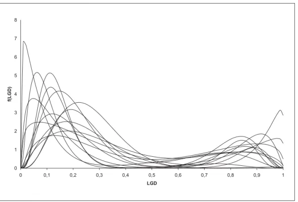
In our case Υ_i is assumed to be beta distributed and _m = 2. Thus Figure 1 shows a possible density function of a mixed distribution resulting from the densities of two beta distributed random variables Υ1 and Υ2 over the interval [0,1].

Figure 1: Mixture density of two beta distributions

The figure shows a possible density function of a mixed distribution resulting from the densities of two beta distributed random variables over the interval [0,1] with ω₁ = 0.8,

p1= 1.5,q1= 11,p2= 12 andq2= 4. 0 1 2 3 4 5 6 0 0,2 0,4 0,6 0,8 1 LGD f(LGD)

right-skewed beta distribution left-skewed beta distribution mixture distribution

The simulation of the LGD is the first step for the simulation of a loan portfolio. Generally this part of our approach can be divided into four steps. At first two beta distributions over the interval5 [0,1] are chosen and, subsequently, the mixture distribution is constructed. Henceforth_nrandom realizations are drawn from the mixture distribution and finally the whole procedure is done_k-times. As a result we get_kloan portfolios with each containing

n obligors characterized by the corresponding LGD.

Beta distributions are defined by the two parameters, here denoted as _pand _q, which are no location and scale parameter itself but in combination. The expected value, the mode, denoted as _γ(_.), and the variance of a beta distributed random variable Υ over [0,1] are

5 _{We chose the interval [0,1] for computational purposes since every LGD distribution can be}

calculated by: E(Υ) = p p+_q (3) γ(Υ) = p−1 p+_q−2 (4) Var(Υ) = p·q (_p+_q+ 1)·(_p+_q)2 (5) Since we want to construct a bimodal distribution from the two beta distributed random variables Υ1and Υ2, where the density of Υ1is assumed to be right-skewed and the density

of Υ2 is assumed to be left-skewed, with corresponding parameters p1, q1 andp2, q2, resp.,

the parameters should fulfill certain assumptions.

First each parameter _p and _q should be greater than one since otherwise the density of these distributions do not exhibit any mode. Furthermore we assume that the ex-pected values E(Υ1) and E(Υ2) are contained in different intervals to ensure a bimodal

density of the mixture distribution and we also assume that Var(Υ1) and Var(Υ2) are

contained in different intervals.6 E(Υ1) should be contained in the interval [0.059,0.3] and

E(Υ2) should lay in [0.7,0.941] where the upper bound of the first interval and the lower

bound of the second one are empirically justified.7 Var(Υ1) is contained in the interval

0_.003_,(1−E(Υ_1+E(Υ1))·(E(Υ1))2

1)

and Var(Υ2) is contained in the interval

0_.003_,E(Υ2₂)₋·(1_E(Υ−E(Υ2))2

2)

. For each portfolio simulated we first need to generate one random mixture distribution by randomly choosing two beta distributions. Therefore, two parameters for each distribu-tion have to be selected by chance. The parameters E(Υ1), E(Υ2) are at first drawn from

the described intervals and the parameters Var(Υ1) and Var(Υ2) are drawn afterwards.

These values are used subsequently for the computation of the parameters_pand_qof each distribution. Assuming_pand_q greater than one, the upper bound of the variance interval depends on a given expected value. The upper bound of Var(Υ1) is derived here, whereas

the upper bound of Var(Υ2) is derived in Appendix 2.

Since Υ1 is assumed to be right-skewed, it follows that q is greater than p. We therefore

rearrange Equation (3) for _q and substitute the value in Equation (5).

Var(Υ1) = p E(Υ1)−p ·p p E(Υ₁)−p+p+ 1 · p E(Υ₁) −p+p 2 = (1−E(Υ1))·(E(Υ1)) 2 p+ E(Υ1) (6)

6 _{A more reasonable parameter for a bimodal distribution might be the modes but due to}

computa-tional simplifications the expected values are chosen instead.

7 _{In Appendix 1 an overview of different studies about LGD distributions with respect to different}

time spans, industrial branches and financial contracts is given. For our intervals the maximum and minimum values of these studies are taken.

Furthermore, the upper bound for the variance is given if _p equals its minimal possible value, namely one, and so we get:

Var(Υ1)< (1−E(Υ1))·(E(Υ1)) 2

1 + E(Υ1) (7)

The lower bounds of the variance intervals are determined simultaneously with the lower bound of the expected value interval in case of Υ1 and the upper bound of the expected

value interval in case of Υ2.

The idea behind the determination of the lower bound of the variance interval is that we want to avoid extremely peaked densities since these densities would result in a very narrow interval for the realizations, namely the LGD in our case. However, such an LGD distribution is not observed in reality and so it seems not suitable for our simulation. Given an expected value, the ratio between the parameters_pand _q remains constant.8 In Appendix 4 it is shown that the variance of a beta distributed random variable decreases for increasing parameters _p and _q given a constant ratio between these parameters. This implies that, given a certain expected value, the variance is higher for lower parameter values _p and _q. However a lower bound for these parameters is given by one. Hence a minimal value for the variance interval corresponds to a minimal expected value. In Table 1 certain combinations of a minimal variance given an expected value are provided. In the whole explanation above, a right-skewed distribution was assumed. For the left-skewed case the parameters _p and _q change their roles and we assume an upper bound for the expected value, but the derivation remains the same.

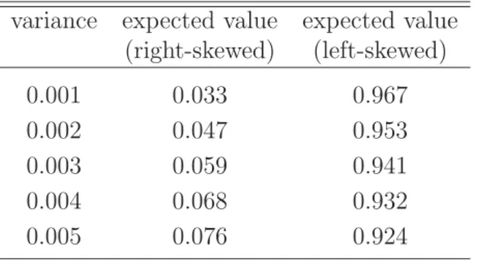
Table 1: Combinations of variances and expected values

The table shows different expected values and corresponding maximum variances (used as the lower bound of the variance intervals).

variance expected value expected value (right-skewed) (left-skewed) 0_.001 0_.033 0_.967 0_.002 0_.047 0_.953 0_.003 0_.059 0_.941 0_.004 0_.068 0_.932 0_.005 0_.076 0_.924

For our purpose a minimum variance of 0.003 is chosen for the interval. A lower variance would result in very peaked densities and a higher variance implies that the minimal ex-pected value for the right-skewed density is above six percent, which is not very meaningful for recovered loans.

Finally the weight _ω1 is randomly selected from the open interval (0.5,1), where ω1 can

be interpreted as a kind of probability of recovery and 1 −_ω1 as a kind of write-off

probability. Thus we implicitly assume that the probability of recovery is always larger than the write-off probability.9

An illustration of possible mixture densities, which result according to the approach de-scribed above, is provided in Figure 2.

Figure 2: Possible mixture densities of two beta distributions

The figure shows possible mixed density functions of two beta distributed random variables over the interval [0,1] according to the approach described earlier.

0 1 2 3 4 5 6 7 8 0 0,1 0,2 0,3 0,4 0,5 0,6 0,7 0,8 0,9 1 LGD f(LGD)

After creating the mixture distribution, the portfolio generation requires that _n realiza-tions from this underlying distribution have to be drawn. In general there are two widely accepted methods to draw realizations from a given distribution in a Monte Carlo sim-ulation. The most famous one is the Inversion Method. Due to the definition of a beta distributed random variable it is not possible to obtain the inverse of the distribution function analytically and this is also true for mixture distributions consisting of beta dis-tributions. Nevertheless we apply this method numerically by dividing the interval [0,1] into 10,001 equidistant points. For each point, _ηi, we compute the value of the mixture distribution function which equals the cumulated probability up to this point according to Equation (2). Subsequently we draw_n realizationsfrom a [0,1]-uniformly distributed

random variable and obtain _n simulated LGDs (_ψi) as a solution of: ψi =F−1 arg max F(ηi) (−_F(_ηi))_>0 (8)

The second widely accepted method is the Acceptance and Rejection Method where the general idea is to find a target probability distribution _T, with given density function

t(_x), from which random realizations can be easily drawn.10 Furthermore the target’s density should be close to the density of the examined distribution, in our case the mixture distribution. However there is no ”simple” distribution which density is close to a bimodal density. Hence when using well-known distributions as the target the algorithm becomes inefficient since there is a great rejection probability resulting from the difference between the two densities. Therefore the numerical Inversion Method described above seems more efficient and reasonable.

3.2

Simulation of Obligor’s Parameters

The second part of this section describes the modelling of the obligor-specific parameters. Therefore we use four LGD-influencing variables. Due to descriptive ease we will constrain the simulation of the obligor-specific parameters to fictitious parameters named _A, _B,

C, and _D. However at the end of this section possible LGD influencing parameters are provided. Via usage of a copula we will also include dependencies between three of the parameters. After the modelling, Section 3.3 will provide the merger of the LGD and the simulated parameter values.

Parameter _A is assumed to be beta distributed with _p=_q = 5. Since _A is truncated on the [0,1]-interval it can be interpreted as a kind of ratio, e.g. a financial statement ratio or another credit-influencing ratio. Furthermore we imply a positive causal relation between

A and the LGD. The second parameter, _B, is normally distributed with _μ = 0_.05 and

σ = 0_.2. This parameter can be interpreted as a profit ratio, e.g. return on investment or return on equity. Thus we imply a negative causal relation between _B and the LGD. Parameter_C is binary distributed where the cut-off point between the two classes is 0.7, i.e. the probability of an observation of the first class is 70 per cent. This parameter can be interpreted as a kind of status variable, e.g. repeated default, existence of collateralization or classification into junior or senior debt. We imply a negative causal relation between

C and the LGD. The last parameter, _D, is beta distributed with _p= 2 and _q= 10. Like the first parameter, _D can be interpreted as a kind of ratio, whereas the causal relation between _D and the LGD is assumed to be negative.

10_{The Acceptance and Rejection Method was introduced by von Neumann (1951). For further}

Regarding the correlation between all parameters, we assume that parameter _A has no causal coherence to any other parameter and thus we assume independency between this parameter and the others. So this means that we can independently draw from the parameter-underlying distribution by using the Inversion Method. The causal coherence between the parameters_B,_C and _Dis assumed to be positive between each of them. For the construction of this dependency, we choose a copula approach.

A copula can be, roughly speaking, regarded as a function that joins or couples multivari-ate distribution functions to their one-dimensional marginal distribution functions and whose one-dimensional margins are uniform.11 More precisely,12

Definition 1. A function _C : [0_,1]n → [0_,1] is a n-copula if it enjoys the following properties:

• ∀ u∈[0_,1] :_C(1_{, . . . ,}1_{, u,}1_{, . . . ,}1) =_u,

• ∀ ui ∈[0,1] :C(u1, . . . , un) = 0 if ∃ j ∈ {1, . . . , n}:uj = 0,

• C is grounded and _n-increasing.

Since the aim of our model is not the analysis of asymmetric dependencies in the pa-rameters, we apply a Gaussian copula and not an Archimedean copula. When using this simulation approach with real historical data one has to be cautious in choosing the appropriate dependency structure, i.e. a Gaussian copula may not be the best fitting dependency model for other parameters.13

Now we introduce the construction principle for our case of a three-dimensional Gaussian copula. First we need the correlation matrix_ρwhich has to be at least positive semidefinite according to the definition of a copula. Our general assumption is a positive dependency between each variable which, however, does not imply the positiv semidefiniteness of

ρ. We construct intervals for each correlation parameter between two variables within the copula since we do not want to have a fixed correlation matrix for all simulated portfolios. Therefore we will draw single correlation parameters from the intervals for each portfolio subject to the constraint that the resulting correlation matrix is at least positive semidefinite. Furthermore we assume that the dependency between parameters

B and _C and the dependency between _C and _D are at least as high as the dependency between parameters_B and_D. Since we demand intervals as large as possible, a non-linear optimization problem according to Appendix 5 has to be solved, resulting in the following correlation matrix, where the first row denotes the dependencies of _B, the second row

11_{See Nelsen (2006), p. 7.}

12_{See Malervergne and Sornette (2006), pp. 103-104.}

denotes the dependencies of_C and the last row denotes the dependencies of _D. ρ= ⎛ ⎜ ⎝ 1 _{ρB,C ρB,D} 1 _ρC,D 1 ⎞ ⎟ ⎠= ⎛ ⎜ ⎝ 1 [0_.5_,0_.75] [0_.125_,0_.5] 1 [0_.5_,0_.75] 1 ⎞ ⎟ ⎠ (9)

The next step in the copula computation is the transformation of three independently standard-normally distributed random variables _{Zi, i} = 1_,2_,3 into three dependent standard-normally distributed random variables _{Xi, i} = 1_,2_,3 using the Cholesky de-composition of _ρ. Hence the dependent variables are given by:

X1 = Z1 X2 = ρB,C·Z1+ 1−_ρ2_B,C·_Z2 X3 = ρB,D·Z1+ ρC,D−ρB,D·ρB,C 1−_ρ2_B,C ·Z2 + 1−_ρ2_B,D −(_ρC,D −_ρB,D·_ρB,C)2·_Z3 (10)

In the next step the three dependent variables are plugged in the distribution function of the standard normal distribution and thus we get three dependent uniformly distributed random variables _{Ui, i} = 1_,2_,3. Finally the _Ui’s are used as the input for the Inversion Method to generate observations from the marginal distributions underlying the copula, e.g. _U3 is used as the input for the inverse beta distribution to generate observations for

parameter _D.14

After this simulation procedure we obtained _k portfolios each comprising _n observations of four obligor parameters. The final step for the portfolio creation is the merger of the four parameters with the simulated LGD value in a systematic manner described in the next part.

3.3

Merging of LGD and Parameters

This part finishes the portfolio creation by combining the four parameters and the LGD into one obligor-specific defaulted loan. The parameters will be matched in a quasi-random procedure where the dependency structure between each parameter and the LGD men-tioned in the prior part is applied. However, we include a stochastic component in this

14_{A further step is needed to generate the copula. The computation of the joint distribution involves}

creating the weighted sum of the inverse of the marginal distributions. Nevertheless we do not need aggregated observations and a meaningful interpretation of this aggregate observation is not given for our case.

matching to obtain a more realistic credit portfolio. The detailed procedure is described in the following.

First we sort the simulated observations of each parameter, including the LGD, and create quintiles. For the parameters in the copula we apply the sorting procedure and quintile creation to the copula values instead of the simulated observations of the marginal distributions. Parameter _A will be matched separately to the LGD since there is no dependency to the other parameters. The matching procedure is done by means of a so called ”double-stochastic matrix”. Due to the disposition of each parameter into quintiles, we will match each quintile of the obligor’s parameter to an LGD quintile according to the specific dependency structure. For the ease of comprehension the matching procedure will be explained for parameters with a negative causal relation to the LGD, e.g. _B. Initially we need a five-by-five matrix_M describing our double-stochastic matrix since we want to match quintiles. Each element of_M,_{mi,j, i, j} = 1_{, . . . ,}5, describes the probability that an observation of the _j-th quintile of (in this example) parameter _B is matched to an observation of the_i-th quintile of the LGD. For completeness reasons of the matching, the row sum has to equal one for all rows, i.e.,

5

j=1mi,j = 1 ∀ i, as well as for the column

sum, i.e.,

5

i=1mi,j

= 1 ∀ _j. A linear program can be solved for the generation of _M and is described in Appendix 6. The resulting matrix for our case is presented in Figure 3 where the probability for each _mi,j is given.

Figure 3: Matrix_M for the matching process

The figure shows the outcome of the linear program according to Appendix 6 presented as the matrixM. 2.5 % 2.5 % 5 % 5 % 5 % 5 % 10 % 10 % 10 % 10 % 10 % 10 % 20 % 20 % 20 % 20 % 20 % 20 % 20 % 20 % 62.5 % 62.5 % 45 % 45 % 40 %

After generation of the matrix, we pick the first observation of the first LGD-quintile. Furthermore a random number _Nr from a uniform-[0,1]-distribution is drawn and com-pared with the cumulated probabilities of the first row of_M. If, e.g., _Nr= 0_.425, the first LGD-observation is matched with an observation of parameter _B of the fifth quintile. This observation is randomly chosen from the fifth quintile and both matched values are deleted from the set of observations. The procedure is repeated _n times for _k portfolios resulting in _n·_k pairs of observations. An obstacle that may occur during the matching process might be a chosen parameter _B quintile which is already empty. In this case, the next plausible quintile is chosen.

The whole procedure described for parameter _B is done for the copula values instead of the realizations of the marginal distributions within the copula. After matching the copula with the LGD, we replace the copula value with the respective observations of the marginal distributions. One has to consider that for a different dependency structure, e.g. for parameter _A, the matrix _M is mirrored around the third column. Finally we obtain_k matrices with each consisting of five columns (LGD and four obligor parameters) and _n rows. Thus each matrix describes a loan portfolio consisting of_n obligors.

As can be seen in Figure 3 the matching probabilities for the assumed relationship between the LGD and the obligor-specific parameters are rather small in the sense that, e.g. for the second, third and fourth quintile the probability for the correct classification assumed is below 50 percent, namely 45 percent for the second and fourth quintile and 40 percent for the third quintile. This matching structure allows for many outliers, which finally leads to a less predictive relationship between the obligor-specific parameters and the LGD. Thus we will refer to this resulting data set as the ”bad data set” in the further sections of this paper. To enhance the general validity of our upcoming estimation model we create a second data set according to the same process described above. However, this data set exhibits a quite higher predictive relationship due to an increase of the probabilities for the correct classification assumed and is in the further proceeding referred to as ”good data set”.15 So both data sets can be used to verify the performance quality of our model and the benchmark models developed in the next Section.

This finishes the simulation part of our paper. We will use the simulated portfolios in the following sections for analyzing different LGD-estimation models. Our simulation ap-proach is different to all existing methods described in the literature to model credit portfolios where the idea is focused on a kind of macroeconomic description of a loan portfolio in the sense of using a superordinated systematic risk factor. Instead our ap-proach is more focused on the idea of the microstructure of the loan portfolio in the sense of using obligor-specific properties. Therefore banks are able to apply this approach to

15_{The corresponding matrix for the matching process for the good data set can be found in Appendix}

get any synthesized number of credit portfolios using historical data to approximate the parameter-underlying distributions. This is especially important if the size of the real credit portfolio is large enough for obtaining the distributions and dependencies of the obligor’s parameters but too small for a decomposition of the portfolio for further anal-yses like modeling, validating and stress testing. Additionally the described approach is adjustable for simulating similar problem sets, e.g., probability of default estimations, rating function derivations or pricing models.

As mentioned before, the portfolio consists of fictitious obligor-specific parameters. A possible LGD-influencing factor might be the rating of the obligor. The rating can be considered as a measure for the default probability of the obligor. Several studies found an empirical evidence for a positive relation between default probability and LGD.16Another LGD-influencing factor is represented by the seniority of a loan. The relationship between seniority and LGD is assumed to be negative since it is obvious that senior loans are served prior to junior loans in case of a bankruptcy. Also the industry and macroeconomic factors that are influenced by the business cycle might affect the LGD as shown in Schuermann (2005).

4

Estimation Model and Benchmark Models

This part introduces the estimation model applied. As our LGD-estimation shall account for the bimodality of the LGD-distribution, we initially need to estimate the parameters of the mixture distribution. Since we assume the LGD-distribution being a mixture of two beta distributions, two commonly used algorithms are introduced for the estimation of the two parameters,_pand _q, of each beta distribution and the weight_ω1. We furthermore

analyze the efficiency and reliability of both algorithms since up to our knowledge this analysis has not been done for this special case of mixture distributions.

4.1

Maximum Likelihood Algorithm

The well-known Maximum Likelihood (ML) algorithm can be used to compute the pa-rameters and weights of a mixture distribution but as we will see shortly the problem may be analytically intractable. The likelihood function for a mixture distribution consisting of two distributions reads as:

LML = n i=1 f(_υi) = n i=1 (_ω1·f1(υi) + (1−ω1)·f2(υi)) (11)

16_{See e.g. Bakshi et al. (2001) and Jokivuolle and Peura (2003). For a detailed literature overview on}

and thus the log likelihood function reads as: log_LML = n i=1 log (_ω1·f1(υi) + (1−ω1)·f2(υi)). (12)

As we assume a mixture consisting of two beta distributed random variables, an analytical solution of the maximization is not possible. Therefore a numerical procedure has to be used where the iterative step of the enhancement of the parameter vector_θ reads as:

θ(k+1) = _θ(k)− ∂2log_LML ∂θ∂θ ₋1 · ∂logLML ∂θ(k) (13)

This approach is the well-known Newton-Raphson method and is considered as a fast and reliable approximation algorithm. Thus we need the first and second (partial) derivatives of the log likelihood function for the gradient and the Hessian inverse. The iterative procedure is repeated until the relative change in the log likelihood function does not exceed a predefined level of tolerance.

4.2

Expectation Maximization Algorithm

The Expectation Maximization (EM) algorithm introduced by Dempster et al. (1977) mainly comprises of two steps, the so called E-step and the M-step. First it is assumed that a data set Υ is observed and contains observations described by some distribution. The data set Υ is assumed to be an uncomplete data set. Therefore the existence of a complete data set Λ = (Υ_,Ξ) is assumed, where Ξ is an additional data set containing the missing information. Ξ is assumed to be random and unobservable. Furthermore a distribution for Λ is assumed as well, which is just the joint distribution of (Υ_,Ξ). Hence the density reads as:

f(_λ|Θ) =_f(_{υ, ξ}|Θ) =_f(_ξ|_υ,Θ)·_f(_υ|Θ)_, (14)

where Θ is the set of distribution parameters that are to be estimated. Finally the complete data likelihood function denoted as_LEM can be set:

LEM =

n

i=1

f(_{υi, ξi}|Θ)_. (15)

In our case of a mixture of two beta distributions, the density of the incomplete data set Υ reads as: f(_υi|Θ) = 2 j=1 ωj·fj(υi|θj), (16)

where Θ = (_ω1, ω2, θ1(= p1, q1), θ2(= p2, q2)) and fj denotes the density of the

right-skewed beta distribution (j=1) or the left-right-skewed beta distribution (j=2). Thus the log likelihood function of the incomplete data set results in:

log_LEM = n i=1 f(_{υi, ξi}|Θ) = n i=1 log ₂ j=1 ωj·fj(υi|θj) . (17)

Since the optimization of the logarithm of a sum is pretty difficult, the above mentioned concept about the existence of additional data simplifies the optimization problem. In our case the additional data set Ξ is defined as:

ξi =

⎧ ⎨ ⎩

1 if observation _ibelongs to the first (right-skewed) beta distribution 2 if observation _ibelongs to the second (left-skewed) beta distribution.

(18)

If the additional data Ξ is known, the log likelihood rearranges to:

log_LEM = n i=1 log ₂ j=1 1{ξi=j}·ωj·fj(υi|θj) , (19)

where still a logarithm of a sum is observable but for every observation just one of the summands remains. The reason is that the observations under the additional information are from mutually exclusive densities, i.e. one observation can only be generated by one density. Thus the logarithm of the remaining summand is just the logarithm of a product.

The problem that the additional data set is not known still remains. However it is assumed that the additional data is random and so by taking the conditional expectation of the complete data log likelihood function with respect to the additional data Ξ (known as the E-Step) we end up with a function only depending on the observable data Υ and the parameters Θ that are to be estimated. For optimizing this function, we need both initial values for the density parameters and the distribution of the additional data for taking the expectation. Therefore the conditional expectation of the _k-th iteration reads as:

EΞlogLEM|Θ(k−1) = EΞ _n i=1 log 1_{ξ(k−1) i =1}·ω (k) 1 ·f1(υi|θ1(k)) +1_{ξ(k−1) i =2}·(1−ω (k) 1 )·f2(υi|θ2(k)) = n i=1 EΞ(1_{ξ(k−1) i =1})·(logf1(υi, θ (k) 1 ) + logω1(k)) +EΞ(1_{ξ(k−1) i =2})· log_f2(υi, θ2(k)) + log(1−ω(1k)) (20)

considered only. So the expectations result in: EΞ 1_{ξ(k−1) i =1} = 1·ω (k−1) 1 ·f1(υi, θ(1k−1)) f(_υi,Θ(k−1)) + 0· ω(2k−1)·f2(υi, θ2(k−1)) f(_υi,Θ(k−1)) = ω (k−1) 1 ·f1(υi, θ1(k−1)) f(_υi,Θ(k−1)) and analogously EΞ 1_{ξ(k−1) i =2} = ω (k−1) 2 ·f2(υi, θ2(k−1)) f(_υi,Θ(k−1)) (21)

Inserting (21) in (20) results in:

EΞlogLEM|Θ(k−1) = n i=1 ω1(k−1)·f1(υi, θ(1k−1)) f(_υi,Θ(k−1)) · log_f1(υi, θ1(k)) + logω1(k) +ω (k−1) 2 ·f2(υi, θ2(k−1)) f(_υi,Θ(k−1)) ·logf2(υi, θ (k) 2 ) +ω (k−1) 2 ·f2(υi, θ2(k−1)) f(_υi,Θ(k−1)) ·log 1−_ω1(k) (22)

The M-step requires the optimization of Θ(k), which includes the parameters_p(₁k)_{, q1}(k)_{, p}(₂k)_{, q2}(k) and _ω(₁k). The resulting estimators are subsequently used again for the next iteration of the EM algorithm. Below we show the derivation of the optimal estimator for_ω1(k), which is just the sum of the posterior probabilities over all observations divided by the number of observations. 0=! ∂EΞ log_LEM|Θ(k−1) ∂ω(1k) = n i=1 ω1(k−1)·f1(υi, θ(1k−1)) f(_υi,Θ(k−1)) · 1 ω(1k) −ω (k−1) 2 ·f2(υi, θ(2k−1)) f(_υi,Θ(k−1)) · 1 (1−_ω(₁k)) n i=1 ω(2k−1)·f2(υi, θ2(k−1))·ω1(k) f(_υi,Θ(k−1))·(1−_ω1(k))·_ω1(k) = n i=1 ω1(k−1)·f1(υi, θ1(k−1))·(1−ω1(k)) f(_υi,Θ(k−1))·(1−_ω1(k))·_ω1(k) n i=1 ω(2k−1)·f2(υi, θ2(k−1)) f(_υi,Θ(k−1)) = n i=1 ω1(k−1)·f1(υi, θ(1k−1)) f(_υi,Θ(k−1))·_ω1(k) − n i=1 ω1(k−1)·f1(υi, θ(1k−1)) f(_υi,Θ(k−1)) n i=1 =f(υi,Θ(k−1)) ω1(k−1)·f1(υi, θ(1k−1)) +ω(2k−1)·f2(υi, θ2(k−1)) f(_υi,Θ(k−1)) = n i=1 ω1(k−1)·f1(υi, θ(1k−1)) f(_υi,Θ(k−1))·_ω1(k) ω1(k) = n i=1 ω(1k−1)·f1(υi,θ(1k−1)) f(υi,Θ(k−1)) n (23)

The estimators for the parameters _p and _q of each distribution in the mixture can be derived analogously. However the derivation of these estimators is not that straightforward since it here involves the derivative of the beta density. Beckman and Tietjen (1978) and others show that it is quite complicated to solve the likelihood equations. We therefore consider the Method of Moments (MM) estimators which read as:

p = _υ· υ s2υ · (1−_υ)−1 q = (1−_υ)· υ s2υ · (1−_υ)−1 , (24)

where_s2 denotes the sample variance and_υ denotes the sample mean. Due to our modifi-cation of using the MM estimators for the parameters_pand _q, we only obtain an adjusted EM (aEM) algorithm instead of the pure EM algorithm. We avoid the usage of numerical derivatives as in the ML algorithm due to computational effort.

The general idea of our simulation is to obtain 1,000 credit portfolios each containing 10,000 creditors with individual LGDs and obligor-specific parameters. We had to repeat the above mentioned algorithms 1,385 times to achieve the required number of portfolios, where the ML algorithm stopped 385 times due to non-convergence and in 197 cases the aEM algorithm did not converge. However, in these cases the ML algorithm did not converge as well. In consequence we can state that in our case the aEM algorithm has better convergence properties than the ML algorithm.

In a next step we look at the reliability of our estimators by comparing the mean squared errors (MSE) over all portfolios for the parameters of the mixture distributions. Table 2 shows the results of this reliability analysis.

Table 2: Parameter reliability analysis

The table provides the mean squared errors of each parameter estimated in the mixture model, namely the two parameters of each beta distribution and the weight.

Algorithm MSE of _p1 MSE ofq1 MSE of p2 MSE ofq2 MSE of ω1

ML 0_.0055 0_.1583 1_.9490 0_.2153 1_.7968·10−4 aEM 0_.0158 0_.3768 10_.8126 0_.3426 1_.7934·10−4

It can clearly be seen that the ML estimators are much more accurate in all parameters than the corresponding aEM estimators except for the estimation of the weighting factor. However the difference between both MSEs is negligible. Resuming the analysis we obtain that the ML algorithm provides more accuracy than the aEM algorithm but at the expense of the convergency properties.17 Due to the relative small values of the MSEs for each

17_{We omit a further statistical analysis due to the clear difference in the MSE values and the number}

parameter, the resulting LGD estimation based on these estimated parameters will only slightly deviate from the ”true” LGD values underlying the simulation.

4.3

Estimation of LGDs with Obligor-Specific Parameters

Now we will explain our complete estimation model in more detail. It generally consists of five steps with small deviations depending on the estimation approach. First the dis-tribution parameters of the mixture disdis-tribution, i.e. _p1, q1, p2, q2 and ω1, are estimated

via either the ML or aEM algorithm. However we only apply the ML algorithm due to the better accuracy in the parameter estimation. The next step requires the computation of the estimated distribution values for both beta distributions over all LGDs (compare Equation (1)). There are two different approaches pursued in the third step. One requires the computation of the mixture distribution values followed by a regression of the trans-formed mixture distribution values on the obligor-specific parameters. The transformation is done due to the bounded nature of the dependent variable and will be discussed in more detail below. The second alternative carried out in this step requires the regression of the transformed single distribution values on the obligor-specific parameters for each beta distribution. Subsequently both estimators of the regressions are weighted with estimated

ω. The fourth step is equal for both alternatives and contains the re-transformation of the estimators into an again bounded estimator for the distribution value of the mixture. Finally the LGDs are estimated via the Inversion Method described at the end of Section 3.1.

Now the single steps are described in more detail. The first step was described in detail in the Sections 4.1 and 4.2. By using the estimated parameter values, the required estimated distribution values can be computed in the second step. The third step first involves the transformation of the estimated distribution values of either the mixture or the single beta distribution values. Two different transformation types are used, namely the logit transformation and the normal transformation. The logit transformation reads as:

y_ilog = log F(υi) 1−_F(_υi) and accordingly

yj,_ilog = log Fj(υi)

1−_Fj(_υi), j = 1,2, (25) and the normal transformation reads as:

yinorm = Φ−1(μ, σ, F(υi))

and accordingly

The argument _υi is the _i-th observation of the realized LGDs, _F(_.) denotes the mixture distribution and _Fj(_.) denotes the single beta distribution. The parameters _μ and _σ are the mean and the standard deviation of the mixture distribution which act as the location and scale parameter in the normal distribution and Φ−1 denotes the inverse distribution function of a standard normally distributed random variable. After the transformation a linear regression of the estimated distribution values for either the mixture distribution or each beta distribution on the obligor-specific parameters is carried out.

In the fourth step, the estimators are either re-transformed in case of the regression in-volving the mixture distribution or the_ω-weighted estimators from each beta distribution are re-transformed. The final step comprises the computation of the LGD via the inverse of the estimated mixture distribution values by applying the Inversion Method according to Equation (8). For future LGD estimations one would skip the first two steps and would just insert the obligor-specific parameters into the regression model of the third step. Afterwards one would proceed with the last two steps.

4.4

Benchmark Models

We will now introduce the before mentioned benchmark models in the way we will apply them in our analysis. Starting with the approach of Hamerle et al. (2006) we first transform the bounded LGDs into an unbounded variable_yHam by the logit transformation:

yHami = log

LGD_i

1−LGD_i. (27)

Afterwards an OLS regression is applied to the transformed LGDs. Since we do not have any time consideration, the panel regression described by Hamerle et al. (2006) is reduced to an OLS regression in our case. The dependent variable _yham is retransformed into an estimation of the LGD.

The second benchmark model is in the style of the LossCalc model by Moody’s KMV described by Gupton and Stein (2005). The assumption underlying the model is an LGD described by just one beta distribution. Therefore a transformation of the LGD is done by normalizing the LGD via a beta transformation:

yKMV_i = Φ−1(_{μ, σ,}Beta(LGD_i))_, (28)

where _μ and _σ are the estimators of the mean and the standard deviation of the beta distribution. Analogously to the fist benchmark model an OLS regression is applied. The

retransformation is done by: LGD_i = Beta−1(_{p, q,}Φ(_yi))_, where p = μ 2_·(1−μ) σ2 −μ q= 1 μ −1. (29)

As a third benchmark model we choose the regression tree model applied to recovery rates proposed by Bastos (2009). Regression trees are nonparametric and nonlinear predictive models and were first introduced by Breiman et al. (1998). The general idea is a clustering according to certain splitting rules of the credit portfolio according to the obligor-specific parameters into more homogeneous, mutually exclusive subportfolios. Logical if-then con-ditions lead to a decomposition of a root node into daughter nodes by a recursive search algorithm.18There are certain splitting rules applicable, where Bastos (2009) refers to the so-called ”maximum deviance reduction” rule. The referring decision measure of this rule is denoted as_DR and reads as:

DR =_σT − μT1

μT ·σT1−

μT2

μT ·σT2, (30)

where _σ and _μ denote the standard deviation and the mean of the nodes named in the subscript,_T denotes the parent node and_T1 and_T2 are the observation set of the daughter nodes. In our case we implemented the model via the MATLAB routine classregtree where the initial tree is reduced to a certain level (deepness of the tree) by the command

prune. The best level is the one that produces the smallest tree that is within one standard error of the minimum-cost subtree.

5

Results

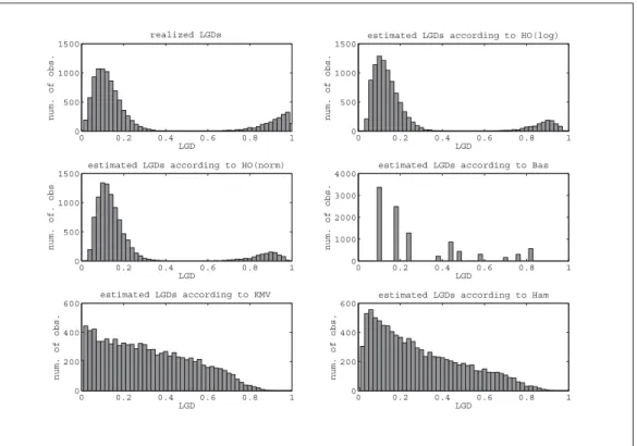
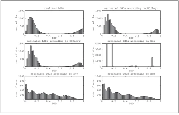
We first define the following abbreviations:

• HOlog: mixture distribution model with logit transformation

• HOnorm: mixture distribution model with normal transformation

• Bas: benchmark model with the approach according to Bastos (2009)

• KMV: benchmark model with the approach according to Gupton and Stein (2005)

• Ham: benchmark model with the approach according to Hamerle et al. (2006).

18_{We omit the technical details of the procedure since it is not in the focus of our paper. For more}

We will refer to these abbreviations in the following parts. The models where the regression is done on the single beta distribution values are not analyzed in more detail since the analysis showed that these models could not exhibit a constant sufficient performance over all portfolios. This may be due to the kind of data, which we cannot check since no real data are available. It may also be due to the kind of regression and transformation process.

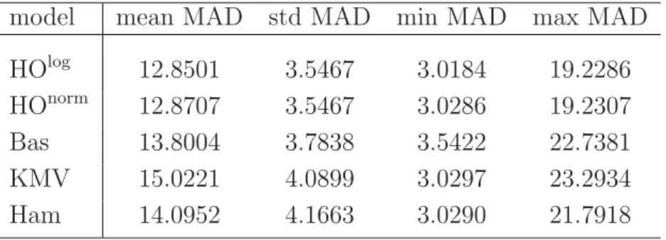
The complete analysis is done for both the good and the bad data set.19 First the mean absolute deviations (MAD) of the estimated LGDs from the realized LGDs are computed for each portfolio and each modelling approach. The minimum, the maximum and the mean MAD for the bad data set are presented in Table 3.

Table 3: Results for the bad data set

The table shows the mean MAD and the standard deviation of the MAD (std MAD) over all portfolios, the minimum MAD, and the maximum MAD for our two models and the three benchmark models for the bad data set. All results are multiplied with a factor 100 so that they can be interpreted as percentage points.

model mean MAD std MAD min MAD max MAD

HOlog 12_.8501 3_.5467 3_.0184 19_.2286 HOnorm 12_.8707 3_.5467 3_.0286 19_.2307 Bas 13_.8004 3_.7838 3_.5422 22_.7381 KMV 15_.0221 4_.0899 3_.0297 23_.2934 Ham 14_.0952 4_.1663 3_.0290 21_.7918

It can be seen that our models are at least one percentage point better than the benchmark models with respect to the mean MAD, which results in an accuracy improvement of at least 6.94 percent (HOnorm vs. Bas) up to 11.28 percent (HOlog vs. KMV). Furthermore the standard deviations of the MAD of our models are also smaller than the ones of the benchmark models. The relative differences between the standard deviations of the MAD between our models and the benchmark models reach from 6.27 percent (HOnorm/log vs. Bas) to 14.87 percent (HOnorm/log vs. Ham). This result is additionally emphasized by the lower maximal values of the MADs.

The results for the good data set are presented in Table 4. In case of the good data set it is obvious that our approaches are still better than the models according to Gupton and Stein (2005) and Hamerle et al. (2006) with respect to the mean MAD. Both approaches offer mean MADs that are at least 16.37 percent lower than the mean MAD of the model proposed by Hamerle et al. (2006). In comparison to KMV our both approaches even

19_{It has to be noted that the KMV model did not work properly in 55 cases of all portfolios. This}

problem arose since the small values obtained after the transformation could not be processed by the computer. These portfolios were only removed for the analysis of the KMV model.

Table 4:Results for the good data set

The table shows the mean MAD and the standard deviation of the MAD (std MAD) over all portfolios, the minimum MAD, and the maximum MAD for our two models and the three benchmark models for the good data set. All results are multiplied with a factor 100 so that they can be interpreted as percentage points.

model mean MAD std MAD min MAD max MAD

HOlog 8_.0929 1_.7000 2_.0748 11_.6390 HOnorm 8_.0730 1_.6723 2_.0884 11_.6298 Bas 7_.5675 1_.4896 2_.1293 11_.9463 KMV 10_.8753 2_.7582 2_.0873 17_.8138 Ham 9_.9110 2_.5897 2_.0988 17_.3259

posses a mean MAD that is more than 22 percent smaller. When comparing the standard deviations of the MADs and choosing the standard deviation of HOlog as the benchmark, we are still more than 34 percent smaller than the model of Hamerle et al. (2006) and more than 38 percent smaller than the KMV model. Thus our models offer a considerably better accuracy in the LGD estimation than both just mentioned benchmark models.

Regarding the model proposed by Bastos (2009) the mean and the standard deviation of the MAD are lower than those of our models. However our models are better in case of considering the extreme values of the MADs. It has to be mentioned that there are some critical points regarding regression trees. One problem is the rigidity of the ap-proach. Since it is a kind of clustering model the continuity of the influencing parameters vanishes and is reduced to a binary decision rule. This means that depending on the branching structure and deepness of the tree an outlier in just one influencing factor may lead to completely misspecified LGDs which may also lead to counterintuitive interpreta-tions. This is especially important when having a data set that offers a weak predictive power of the influencing factors on the LGD. A second disadvantage of the regression tree model compared to a straight-forward regression approach is the inflexibility. This means that regular regression approaches can use nearly every functional dependency between the explanatory variables and the dependent variable and even between the explanatory variables themselves.

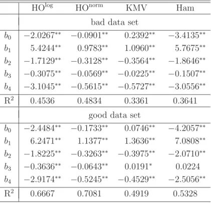
We exemplarily choose a portfolio to illustrate the regression results and the corresponding estimated LGD distributions. This is done for the good data set as well as for the bad data set. In Table 5 the regression coefficients, their significance and the coefficient of determination for our models, the KMV model and the model according to Hamerle et al. (2006) are presented. The regression coefficients are obtained from the linear regression

ˆ

yi =b0+b1·Ai+b2·Bi+b3·Ci+b4·Di, where A, B, C, andD are the obligor-specific

value of the realized LGD. Since the regression tree model proposed by Bastos (2009) does not exhibit any functional relationship we could not obtain any regression coefficients nor a coefficient of determination and is therefore excluded from the table. The regression tree for the good data set of the exemplarily chosen portfolio can be found in Appendix 8.

Table 5: Estimation results for the randomly chosen portfolio

The table shows the regression coefficients for the four regres-sion models according to the equation ˆy_i=b₀+b₁·A_i+b₂·B_i+

b3·Ci+b₄·D_i. Furthermore the coefficient of determination is given as well. A double asterisk indicates significance on the one percent level and a single asterisk indicates significance on the five percent level.

HOlog HOnorm KMV Ham bad data set

b0 −2.0267∗∗ −0.0901∗∗ 0.2392∗∗ −3.4135∗∗ b1 5.4244∗∗ 0.9783∗∗ 1.0960∗∗ 5.7675∗∗ b2 −1.7129∗∗ −0.3128∗∗ −0.3564∗∗ −1.8646∗∗ b3 −0.3075∗∗ −0.0569∗∗ −0.0225∗∗ −0.1507∗∗ b4 −3.1045∗∗ −0.5615∗∗ −0.5727∗∗ −3.0556∗∗ R2 0_.4536 0_.4834 0_.3361 0_.3641 good data set

b0 −2.4484∗∗ −0.1733∗∗ 0.0746∗∗ −4.2057∗∗ b1 6.2471∗∗ 1.1377∗∗ 1.3636∗∗ 7.0808∗∗ b2 −1.8225∗∗ −0.3263∗∗ −0.3975∗∗ −2.0710∗∗ b3 −0.3636∗∗ −0.0643∗∗ 0.0191∗ 0.0224 b4 −2.9174∗∗ −0.5245∗∗ −0.4529∗∗ −2.5056∗∗ R2 0_.6667 0_.7081 0_.4919 0_.5328

The table shows that all regression coefficients are highly significant for all models regard-ing the bad data set. The influence direction of the obligor-specific parameters (indicated by the sign of the coefficients) is the same for all models and the same to the one pro-posed by our simulation. Furthermore the coefficients of determination are higher for our approaches compared to the benchmark models but they all are below 0.5. Regarding the good data set the regression coefficients are again always significant and exhibit the assumed direction of influence of the obligor-specific parameters on the LGD for our ap-proaches. This is also true for both benchmark models regarding the parameters _A, _B, and_D. However parameter_C exhibits the contrary direction of influence on the LGD but is not significant for the model according to Hamerle et al. (2006). The coefficients of de-termination have increased for all models whereas our models still offer higher coefficients of determination.