2012
Efficient estimation in missing data and survey
sampling problems
Sixia Chen
Iowa State UniversityFollow this and additional works at:
https://lib.dr.iastate.edu/etd
Part of the
Statistics and Probability Commons
This Dissertation is brought to you for free and open access by the Iowa State University Capstones, Theses and Dissertations at Iowa State University Digital Repository. It has been accepted for inclusion in Graduate Theses and Dissertations by an authorized administrator of Iowa State University Digital Repository. For more information, please [email protected].
Recommended Citation
Chen, Sixia, "Efficient estimation in missing data and survey sampling problems" (2012).Graduate Theses and Dissertations. 12950.
by
Sixia Chen
A dissertation submitted to the graduate faculty in partial fulfillment of the requirements for the degree of
DOCTOR OF PHILOSOPHY
Major: Statistics
Program of Study Committee: Jae Kwang Kim, Co-major Professor Wayne A. Fuller, Co-major Professor
Zhengyuan Zhu Nordman Dan
Cindy L. Yu
Iowa State University Ames, Iowa
2012
DEDICATION
I would like to dedicate this thesis to my parents and my wife without whose support I would not have been able to complete this work. I would also like to thank my friends and family for their loving guidance and financial assistance during the writing of this work.
TABLE OF CONTENTS
LIST OF TABLES . . . vi
LIST OF FIGURES . . . vii
ACKNOWLEDGEMENTS . . . viii
ABSTRACT . . . ix
CHAPTER 1. GENERAL INTRODUCTION . . . 1
CHAPTER 2. SEMI-PARAMETRIC INFERENCE WITH A FUNCTIONAL-FORM EMPIRICAL LIKELIHOOD . . . 4
2.1 Introduction . . . 4 2.2 Main Results . . . 7 2.3 Extension . . . 11 2.4 Computational Aspects . . . 12 2.5 Simulation Study . . . 14 2.6 Conclusions . . . 16
CHAPTER 3. A UNIFIED THEORY ON EMPIRICAL LIKELIHOOD METH-ODS WITH MISSING DATA AND SURVEY SAMPLING . . . 20
3.1 Introduction . . . 21
3.2 Basic setup . . . 23
3.3 Estimation with known response probability . . . 27
3.4 Estimation with unknown response probability . . . 30
3.5 Nonparametric estimation of the response mechanism . . . 33
3.7 Simulation Study . . . 38
3.7.1 Simulation One . . . 38
3.7.2 Simulation Two . . . 40
CHAPTER 4. POPULATION EMPIRICAL LIKELIHOOD FOR NON-PARAMETRIC INFERENCE IN SURVEY SAMPLING . . . 45
4.1 Introduction . . . 46
4.2 Population empirical likelihood . . . 47
4.3 Main results . . . 50
4.4 Extension to rejective Poisson sampling . . . 56
4.5 Combining information from two independent surveys . . . 61
4.6 Simulation Study . . . 63
4.6.1 Simulation One . . . 63
4.6.2 Simulation Two . . . 65
4.7 Concluding remarks . . . 66
CHAPTER 5. TWO-PHASE SAMPLING FOR PROPENSITY SCORE ES-TIMATION IN VOLUNTARY SAMPLES . . . 70
5.1 Introduction . . . 70
5.2 Basic Setup . . . 72
5.3 Main Results . . . 74
5.4 Extension to non-nested two-phase sampling . . . 78
5.5 Simulation Study . . . 82
5.5.1 Simulation One . . . 82
5.5.2 Simulation Two . . . 83
5.6 Empirical Study . . . 84
5.7 Concluding Remarks . . . 87
CHAPTER 6. FUTURE RESEARCH TOPICS . . . 90
6.1 Jackknife empirical likelihood for inference with imputed data . . . 90
6.3 Inference with parametric fractional imputation . . . 94
APPENDIX A. PROOFS FOR CHAPTER 2 . . . 97
APPENDIX B. PROOFS FOR CHAPTER 3 . . . 106
APPENDIX C. PROOFS FOR CHAPTER 4 . . . 116
APPENDIX D. PROOFS FOR CHAPTER 5 . . . 125
LIST OF TABLES
2.1 Monte Carlo relative efficiency of the point estimators. . . 18
2.2 Power comparisons for testingH0 :ρ= 0 . . . 19
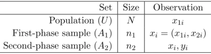
3.1 Data structure for two-phase sampling . . . 36
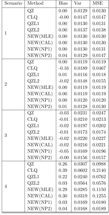
3.2 Biases, Variances and Mean squared errors (MSE) of the estimators
under four different scenarios in simulation one. . . 43
3.3 The Monte Carlo biases, variances, and the mean squared errors (MSE)
of the point estimators in simulation two. . . 44
4.1 Monte Carlo biases, variances, and mean squared errors of the point
estimators. . . 68
4.2 Coverage rate and average length comparison for Wald’s and Wilk’s
type 95% confidence intervals of proposed POEL2 method. . . 69
4.3 The Monte Carlo biases, variances, and the mean squared errors (MSE)
of the point estimators in Simulation Two. . . 69
5.1 Simulation results of the point estimators for θ1 and θ2 in Simulation
One. . . 88
5.2 Simulation results of the point estimators forθ in Simulation Two. . . 88
5.3 Estimated coefficients in the propensity model . . . 89
LIST OF FIGURES
2.1 Parameter estimations versus penalty parameter. . . 17
ACKNOWLEDGEMENTS
I would like to take this opportunity to express my thanks to those who helped me with various aspects of conducting research and the writing of this thesis. First and foremost, Dr. Jae Kwang Kim for his guidance, patience and support throughout this research and the writing of this thesis. His insights and words of encouragement have often inspired me and renewed my hopes for completing my graduate education. I am particularly grateful to Dr. Wayne A. Fuller for his helpful comments and suggestions. I would also like to thank my committee members for their efforts and contributions to this work.
ABSTRACT
The thesis consists of four research papers. The first paper deals with general theory for empirical likelihood under the standard setup. Instead of maximizing the empirical likelihood function, a functional-form approach is proposed to generalize the theory of empirical likelihood and to achieve computational efficiency. The second paper deals with an empirical likelihood approach for missing data. The proposed method uses a partial likelihood for the respondents and theories are developed for both a parametric response model and a nonparametric response model. Also, the proposed method is extended to two-phase sampling where the first-phase sample is obtained by complex survey sampling. The third paper deals with empirical likeli-hood in the survey sampling setup. In the proposed method, called the population empirical likelihood method, the empirical likelihood function is defined for the finite population and the sampling design is incorporated into one of the constraints in the optimization problem. The proposed method is quite useful when combining information from several independent surveys. The fourth paper proposes a novel application of the capture-recapture experiment to estimate the propensity score for nonignorable nonresponse. The proposed method can be used to reduce the selection bias associated with voluntary sampling.
CHAPTER 1. GENERAL INTRODUCTION
Hartley and Rao (1968) introduced the empirical likelihood (EL) approach under the name of “scale load”. Owen (1988,1990) brought the EL method to standard statistical problems. For a comprehensive overview of EL method, see Owen (2001). Chen and Hall (1993) extended the EL method to inference for quantiles. Qin and Lawless (1994) extended the EL method to inference for parameters defined by some general estimating equations. DiCiccio et al. (1991) and Chen and Cui (2006) used bartlett correction techniques to improve the convergence rate of empirical likelihood ratio. The application of EL method in time series has been considered by Kitamura (1997), Nordman et al. (2007) and others. Recently, Hjort, McKeague and Van Keilogom (2009), Chen, Peng and Qin (2009) and Tang and Leng (2010) showed that the EL method continues to work when data dimensionality is growing. Newey and Smith (2004) proposed generalized empirical likelihood (GEL) which extended the scope of the traditional EL method. In chapter 2, we propose a different extension by using the functional-form empirical likelihood (FEL) method. The basic idea is to generalize the form of the EL weight or of the objective function. We prove the first order equivalence between our proposed estimator and the traditional EL estimator. The proposed estimator has certain advantages in terms of computation and choice of weights.
Missing data happens frequently in observational studies. If the missing mechanism is completely missing at random (CMAR) in the sense of Rubin (1976), we can safely remove the missing part of the data. However, if the response mechanism is missing at random (MAR) or not missing at random (NMAR), we may not ignore the missing data in order to produce efficient and consistent estimates. There are two main approaches for inference with missing data: Imputation and Propensity Score Weighting. Wang and Rao (2002) and Wang and Chen (2009) considered combining EL and imputation methods for inference with data missing
at random. Alternatively, Qin, Leung and Shao (2002) proposed the EL method to deal with nonignorable missing data by using the propensity score method. Qin and Zhang (2007) applied the EL method in missing response problems. Chen, Leung and Qin (2008) proposed constructing two different empirical likelihood method with data MAR. Most recently, Qin et al. (2009) provided the complete EL method for missing covariate problem. The literature is somewhat sparse for modeling the response mechanism nonparametrically. Cheng (1994) discussed some asymptotic properties of the mean estimator based on the kernel regression method under ignorable missing data. Recently, Kim and Yu (2011) extended the approach of Cheng (1994) to handle nonignorable nonresponse. Xue (2009) discussed an empirical likelihood method for linear models using the weights computed from a nonparametric model where the kernel regression method is used to estimate the response model. Da Silva and Opsomer (2009) considered another type of nonparametric response probability estimator using local polynomial regression. Hirano et al (2003) and Cattaneo (2010) discussed semiparametric efficiency of the nonparametric response propensity estimators in the context of estimating average treatment effect in econometrics. In chapter 3, we propose a response EL method which can be used to handle both survey sampling and missing data problems. Specifically, we propose estimating the propensity score nonparametrically in the EL method. By doing this, the semi-parametric lower bound can be achieved automatically.
The use of the EL method for a finite population parameter was first considered by Chen and Qin (1993), but their method is only applicable under simple random sampling (SRS). Chen and Sitter (1999) proposed pseduo empirical likelihood (PEL) which can be used to deal with complex survey data. Wu and Rao (2006) constructed a likelihood ratio-based confidence interval for the population mean by using PEL. For the most recent development of PEL,
see Rao and Wu (2009). The likelihood ratio property is the most attractive property of
the EL method. The corresponding confidence region has several advantages compared to the normal approximation (NA) confidence region. These include better coverage rate, shape respecting, and transformation invariance. However, the PEL ratio converges to a scaled chi-squred distribution instead of the standard chi-chi-squred distribution. The scale factor needs to be estimated and it often depends on the complex sampling design. In addition, the PEL
estimator is not equivalent to the design optimal estimator. To avoid those drawbacks, we propose using the population empirical likelihood (POEL) estimator in chapter 4. The POEL likelihood ratio converges to the standard chi-squred distribution; the proposed estimator is equivalent to the design optimal estimator and the POEL method can combine several sources of auxiliary information.
A voluntary sample is a self-selected sample whose first order inclusion probabilities are unknown. The most popular method for the inference for a voluntary sample is propensity score weighting. Rosenbaum and Rubin (1983) and Rosenbaum (1987) proposed using propensity scores to estimate treatment effects in observational studies. Duncan and Stasny (2001) used the propensity score method to control coverage bias in telephone surveys. Lee (2006) applied the propensity score method to a volunteer panel web survey. Lee and Valliant (2009) and Valliant and Dever (2011) considered the propensity score method for a web-based voluntary sample. All of these studies assumed an ignorable selection mechanism. However, we often confront the case where the selection mechanism does depend on the study variable itself. In chapter 5, we propose a novel two-phase approach for estimators with a voluntary sample. The proposed method can be extended to handle a non-nested two-phase voluntary sample. The auxiliary information can be incorporated via the generalized method of moment (GMM).
We organize the thesis as followings. In chapter 2, we present the new functional form empirical likelihood (EL) method; We proposed a unified theory of using the EL method in missing data problems in chapter 3; In chapter 4, we propose using the population empirical likelihood (POEL) method for inference with survey data; In chapter 5, a novel approach is proposed for inference in the voluntary sample problem. Future works are presented in chapter 6. Technical details are presented in the appendixes.
CHAPTER 2. SEMI-PARAMETRIC INFERENCE WITH A FUNCTIONAL-FORM EMPIRICAL LIKELIHOOD
A paper submitted to theJournal of the Korean Statistical Society
Sixia Chen and Jae Kwang Kim
Abstract
A functional-form empirical likelihood method is proposed as an alternative for the empirical likelihood method. The proposed method has the same asymptotic properties as the empirical likelihood method but has more flexibility in choosing the weight construction. Also, some computational efficiency can be gained. Because it enjoys the likelihood-based interpretation, the profile likelihood ratio test has a chi-square limiting distribution. Some computational details are also discussed, and results from limited simulation studies are presented.
Key Words: Exponential tilting, Generalized method of moments, Nonparametric maximum likelihood method, Profile likelihood ratio test.
2.1 Introduction
The empirical likelihood method, proposed by Owen (1988, 1990), provides a useful tool for obtaining nonparametric confidence regions for statistical functionals. Even though the empirical likelihood method is a nonparametric approach in the sense that it does not require a parametric model for the underlying distribution of the sample observation, the empirical likelihood method enjoys some of the desirable properties of the likelihood-based method. Us-ing a nonparametric likelihood function, the empirical likelihood method can easily incorporate
known constraints on parameters and also incorporate prior information on parameters. For example, Chen and Qin (1993) and Qin (2000) discuss combining information using the em-pirical likelihood. A comprehensive overview of the emem-pirical likelihood method is provided by Owen (2001).
We consider an extension of the empirical likelihood method by providing a class of non-parametric estimators that have the same asymptotic properties as the empirical likelihood method. In particular, instead of assuming a nonparametric likelihood, we consider a gen-eralization of the empirical likelihood that uses a functional-form likelihood function in the likelihood maximization. The class of functional-form likelihood function contains the empir-ical likelihood function as a special case. The functional-form likelihood approach provides several useful alternatives to the classical empirical likelihood method in the sense that some of the computational difficulty of the empirical likelihood method can be avoided, and more clear insights can be obtained from the empirical likelihood method.
Let z1,· · · , zn be n independent realizations of a vector-valued random variable Z with a distribution functionF(z) that is completely unspecified. In the empirical likelihood approach, we consider a class of distribution functions, F1 ⊂ F, that have support on {z1, .· · · , zn}.
Thus, the elements inF1 can be written as
Fw(x) = n X i=1 wiI(zi ≤x) with Pn
i=1wi = 1 and wi > 0, where I(zi ≤ x) takes the value one if zi ≤ x and takes the
value zero otherwise. The parameter wi is the amount of point mass that unit zi represents
in the population. We are interested in making an inference about θ0 that is defined as a
unique solution toE{U(Z;θ)}= 0, whereU(Z;θ) is anr-dimensional vector of some function
U(Z;θ) known up to θand the dimension ofθequalsp≤r. Hansen (1982) and Imbens (1997)
considered this over-identified situation in the context of a generalized method of moments in econometrics.
In this setup, Qin and Lawless (1994) considered the empirical likelihood estimator of θ0
that can be obtained by maximizing
n
X
i=1
subject to
n
X
i=1
wi{1, U(zi;θ)}= (1,0). (2.2)
Note that (2.2) is equal to the condition E{U(Z;θ)} = 0 for F ∈ F1. Using the Lagrange
multiplier method, the empirical likelihood estimator can be obtained by maximizing
le(θ) = n
X
i=1
ln{wi(θ)}, (2.3)
wherewi(θ) is of the form
wi(θ) = 1 n 1 1 + ˆλTθU(zi;θ) (2.4) and ˆλθ satisfies the second equation of (2.2). Qin and Lawless (1994) showed that the empirical likelihood estimator satisfies
2nle(ˆθ)−le(θ0)
o
→dχ2p (2.5)
where ˆθis the empirical likelihood estimator. The result (2.5) is often called the Wilk’s theorem for empirical likelihood and is quite useful in obtaining confidence regions for θ0.
The weight (2.4) used to compute the empirical likelihood estimator can be expressed as
wi(θ,λˆθ) = mnˆλTθU(zi;θ) o Pn j=1m n ˆ λT θU(zj;θ) o, (2.6)
wherem(x) = 1/(1−x) and ˆλθ = ˆλ(θ;z1,· · · , zn) satisfies n
X
i=1
wi(θ,ˆλθ)U(zi;θ) = 0. (2.7)
The Lagrange multiplier ˆλθ = ˆλ(θ;z1,· · ·, zn) is completely determined by (2.7). We assume that, for given θ, the solution ˆλθ to (2.7) is unique. The unique solution exists for any given θ if 0 is inside the convex hull of the points U(z1;θ),· · ·, U(zn;θ).
We consider an extension of the empirical likelihood estimator by allowing m(x) in (2.6) to
be some smooth function other thanm(x) = 1/(1−x). The proposed estimator can be called
the functional-form empirical likelihood (FEL) estimator because it uses a known function
m(x) in computing the weights in the FEL estimator. For example, the exponential tilting
(ET) estimator considered in Kitamura and Stutzer (1997) and Schennach (2007) is the same
estimator over the empirical likelihood (EL) estimator based on Monte Carlo investigation and analytic comparison using higher order asymptotic expansion. In this paper, we discuss some asymptotic properties for the FEL estimator. In particular, asymptotic normality and a version of Wilk’s theorem for the FEL estimator are established. We found that the asymptotic results in Qin and Lawless (1994) are special cases of the general results in this paper. The results in this paper can also be used to make inferences for other types of FEL estimators, including the ET estimator.
The main results are presented in Section 2. Some extensions are introduced in Section 3 to illustrate possible theoretical results of the proposed FEL estimator. In Section 4, the underlying algorithm is discussed. Results from a limited simulation study are presented in Section 5 and concluding remarks are made in Section 6.
2.2 Main Results
Based on the functional form of the FEL weights in (2.6), we can define a functional-form
empirical log-likelihood function
l(θ) =l(θ,λˆθ) = n X i=1 lnωi(θ,ˆλθ) = n X i=1 ln ( mi(θ,λˆθ) Pn i=1mi(θ,ˆλθ) ) (2.8)
where mi(θ,λˆθ) = m{λˆTθU(zi;θ)} for some function m(·) and ˆλθ satisfies (2.7). The
log-likelihood function in (2.8) is a parametric form in the sense that the likelihood function is
known except for some unknown parameter (θ, λ). The computation for optimization using
(2.8) is generally simpler than the computation using the nonparametric likelihood (2.1) since
the parameter space is reduced from n to p+r. The parameter λ is used to facilitate the
computation for constrained optimization. Furthermore, the log-likelihood function (2.8) does
not directly use any distributional assumptions. Thus, the nature of the maximum likelihood
estimator using (2.8) is still nonparametric in the sense that it is valid without assuming any
distributional assumptions. The only assumption we use isE{U(Z;θ0)}= 0.
Let ˆθbe the solution that maximizesl(θ,λˆθ) in (2.8). Let ˆQ1(θ, λ) =Pni=1ωi(θ, λ)U(zi;θ) and ˆQ2(θ, λ) ≡ n−1dl(θ,λˆθ)/dθ. The solution ˆθ and its corresponding λ-value, denoted by
ˆ
λ= ˆλ(ˆθ), satisfies ˆQ1(ˆθ,λˆ) = 0 and ˆQ2(ˆθ,ˆλ) = 0. The solution ˆθis called the FEL estimator of
θ0. For simplicity of notation, letγ = (θ, λ) and ˆγ = (ˆθ,λˆ). Also, let ˆQ(γ) = ( ˆQ1(γ),Qˆ2(γ)).
To discuss the asymptotic properties of the FEL estimator, we assume the following condi-tions:
(C1) The solution θ0 toE{U(Z;θ)}= 0 is unique.
(C2) In the weight function (2.6), the function m(x) is always positive and has continuous
second-order derivatives atx= 0 withm(0) =m0(0) = 1.
(C3) The partial derivative ˙U(θ) =∂U(θ)/∂θ is a continuous function ofθin the compact set
Aand θ0 ∈ Aalmost surely.
(C4) The random functions ˆQ(γ) converge uniformly in probability to Q(γ) = EnQˆ(γ)o in the compact setB and γ0 ∈ B,where γ0 = (θ0,0).
The following theorem provides the consistency of the FEL estimator.
Theorem 2.2.1 Assume that conditions (C1)-(C4) hold. Assume that the solution (ˆθ,λˆ) to
ˆ
Q1(θ, λ) = 0 andQˆ2(θ, λ) = 0 is uniquely determined. Then, the solution (ˆθ,ˆλ) satisfies
p lim
n→∞ (ˆθ,
ˆ
λ) = (θ0,0) (2.9)
where θ0 is a unique solution to E{U(Z;θ)}= 0.
In the special case of the empirical likelihood method, Qin and Lawless (1994) also proved
(2.9). The proof of Theorem 2.2.1, which is different from that of Qin and Lawless (1994), is
presented in Section A of Appendix A.
Theorem 2.2.2 In addition to the conditions of Theorem 2.2.1, assume that
(C5) ∂2U(z, θ)/(∂θ∂θT) is continuous atθ in the compact set A almost surely.
(C6) ||U(Z;θ)||3, ||∂U(Z;θ)/∂θ||, and ||∂2U(Z, θ)/(∂θ∂θT)|| are bounded by some integrable
(C7) The r ×p matrix E{∂U(Z;θ0)/∂θ} has full column rank p. Also, V ar{U(Z;θ)} is
positive definite in the compact set A.
Then, we have √ n ˆ θ−θ0 ˆ λ−0 → dN(0,V) (2.10) where V= V1 0 0 V2 where V1= E(∂U ∂θ) T(EU UT)−1E(∂U ∂θ) −1 and V2 = E(U UT) −1 I−E(∂U ∂θ)V1E( ∂U ∂θ) T[E(U UT)]−1 .
The proof of Theorem 2.2.2 is presented in Section B of Appendix A. Using Theorem 2.2.2, we
can construct a Wald-type confidence interval forθ0. The asymptotic varianceV1of
√
n(ˆθ−θ0)
can be consistently estimated by
( n X i=1 wiU˙ zi; ˆθ )T( n X i=1 wiU zi; ˆθ Uzi; ˆθ T )−1( n X i=1 wiU˙ zi; ˆθ ) −1 ,
wherewi =wi(ˆθ,λˆ) is the final FEL weight in (2.6) evaluated at ˆθand ˆλ.
By Theorem 2.2.2, asymptotic variance of the FEL estimator can be derived. For example, ifzi = (xi, yi)T andµx =E(x) is known, the FEL estimator ofθ=E(y) can be obtained using ˆ
θ = Pn
i=1mˆiyi/Pni=1mˆi with ˆmi = m{λˆ(xi−µx)} where ˆλ satisfies Pin=1mˆi(xi −µx) = 0. The asymptotic variance of ˆθis equal ton−1V(y)
1−ρ2 whereρis the correlation coefficient
of x and y in the population. Note that the asymptotic variance is equal to the asymptotic
variance of the regression estimator ˆ
θreg = ¯y+SyxSxx−1(µx−x¯) (2.11)
and so the FEL estimator in this setup is asymptotically equivalent to the regression
bivariate normality assumption (Anderson, 1957). The asymptotic variance V1 is equal to
the semiparametric lower bound discussed in Chamberlain (1987) and so the FEL estimator achieves semiparametric efficiency.
Theorem 2.2.3 The functional-form empirical likelihood ratio statistic for testingH0 :θ=θ0
is
W(θ0) =l(ˆθ)−l(θ0) (2.12)
where l(θ) is given by (2.8). Under the assumption of Theorem 2.2.1,we have that
2W(θ0)→dχ2p (2.13)
as n→ ∞,when H0 is true.
Theorem 2.2.3, which can be called the Wilk’s theorem for FEL method, shows that the FEL log-likelihood in (2.8) can be used to construct a confidence interval based on the likelihood
ratio statistics (2.12) as in the parametric likelihood method. In the following corollary, we
show that the FEL method can be used to construct a profile of likelihood ratio confidence intervals. The proofs of Theorem 2.2.3 and Corollary 2.2.1 are presented in Sections C and D of Appendix A, respectively. Results similar to Corollary 2.2.1 are also presented in Qin and Lawless (1994) in the context of empirical likelihood method, but we presents a different proof of the corollary.
Corollary 2.2.1 Let θT = (θ1, θ2)T,where θ1 and θ2 areq×1 and(p−q)×1 vectors,
respec-tively. ForH0:θ1 =θ01,the profile generalized empirical likelihood ratio test statistic is defined
by
W2 =l(ˆθ1,θˆ2)−l(θ10,θˆ02) (2.14)
where θˆ02 maximizes l(θ10, θ2) with respect toθ2. Then, under H0,we have that
2W2→dχ2q
Remark 2.2.1 The FEL method could be called a generalized empirical likelihood method be-cause it is essentially a generalization of the empirical likelihood method using functional-form weight function. The term “generalized empirical likelihood”, however, was already used by Smith (1997) and Newey and Smith (2004) to denote another type of extension to empirical likelihood method in econometrics using a saddle point optimization problem. Our method is different from the GEL method because we do not have to specify the objective function for sad-dle point computation and we have only to directly specify the functional-form for the weights in FEL estimators.
2.3 Extension
The log-likelihood function in (2.8) can be viewed as a negative divergence function between
1/n and wi. Instead of using a divergence function based on the log-likelihood (2.8), one can
also consider a more general class of divergence functions. Specifically, we consider a class of divergence functions based on power-divergence statistics, proposed by Cressie and Read (1984), CR(α) = 2 α(α+ 1) n X i=1 1/n ωi α −1 . (2.15) Note thatCR(0) =−2Pn
i=1log(nωi),which is the log-likelihood function in (2.6) andCR(−1) =
2Pn
i=1nωilog(nωi),which is often called the Kullback-Leibler divergence measure.
The results in Section 2 show that the choice of weight function is not critical because the resulting estimators are all asymptotically equivalent. Surprisingly, we show in this section that the choice of the objective function is not critical either. The results presented here are an
extension of Baggerly (1998) to the case whenθis defined through the solution to an estimating
equation.
Theorem 2.3.1 Let Qˆ1(θ, λ) = Pin=1ωiU(zi;θ) and Qˆ2(θ, λ) = n−1dl3(θ, λ)/dθ where ωi is
defined in (2.6) and l3(θ, λ) =− 1 α(α+ 1) n X i=1 {ωi(θ, λ)n}−α−1 . (2.16)
Suppose that (ˆθ,λˆ) is the solution of Qˆ1(θ, λ) = 0 and Qˆ2(θ, λ) = 0. Then under conditions
stated in theorem 2.2.1 and theorem 2.2.2, we have
√ n ˆ θ−θ0 ˆ λ → dN(0, V) (2.17)
where V is defined in (2.10). Also, the generalized empirical likelihood ratio statistic for testing
H0:θ=θ0 satisfies
2nl3(ˆθ)−l3(θ0)
o
→dχ2p (2.18)
where l3(θ) is given by (2.16).
Theorem 2.3.1 is a general result in the sense that, for the special case of α= 0 in (2.15),
it leads to Theorem 2.2.2 and Theorem 2.2.3. Also, for the special case ofα =−1, we have the
following result. Its proof is very similar to that of Theorem 2.3.1 and is not presented here.
Corollary 2.3.1 Let l2(θ) = −Pni=1nωilog(nωi) and assume that θˆ maximizes l2(θ). Then
we have 2 n l2(ˆθ)−l2(θ0) o →dχ2p,
and θ0 is the true value of θ.
2.4 Computational Aspects
The FEL estimator that maximizes the objective function (2.8) subject to the constraint
(2.7) could be viewed as a standard optimization problem in the (θ, λ) space of dimension
p +r. However, as shown in Section A of Appendix A, the probability limit Q2(θ, λ) of
ˆ
Q2(θ, λ) satisfies Q2(θ,0) = 0 for all θ. Thus, standard approaches to solving the systems
of equations ˆQ1(θ, λ) = 0 and ˆQ2(θ, λ) = 0 can have erratic behavior in the neighborhood of
λ= 0.
To avoid this numerical problem, we consider an approach using a penalty term used in the ridge regression method, as was also considered by Imbens, Spady, and Johnson (1998). The objective function with a penalty term can be expressed as
wherel(θ, λ) is the original objective function, such as (2.8) or (2.16), andKis a scalar penalty
term that makes the optimization problem locally convex, andW is somer×rpositive definite
matrix. Note that ˆQ∗2(θ, λ) =n−1∂l∗(θ, λ)/∂θ can be written ˆ
Q∗2(θ, λ) =Q2(θ, λ)−K·n−1Q˙1θ(θ, λ)TWQˆ1(θ, λ),
where ˙Q1θ(θ, λ) =∂Qˆ1(θ, λ)/∂θ. Thus, for sufficiently large K =O(n), we have
Q∗2(θ,0)6= 0 forθ6=θ0 and Q∗2(θ0,0) = 0, (2.20)
whereQ∗2(θ, λ) is the probability limit of ˆQ∗2(θ, λ). Property (2.20) follows because
Q∗2(θ, λ) =Q2(θ, λ) +C(θ, λ)Q1(θ, λ)
for some matrixC(θ, λ),andQ1(θ, λ) satisfies (2.20). Once the solution
ˆ θ∗,λˆ∗that maximizes l∗(θ, λ) in (2.19) is obtained, we solve ˆ Q1 ˆ θ∗, λ= n X i=1 mnλTU(zi; ˆθ∗) o U(zi; ˆθ∗) = 0 (2.21)
forλto get the final solution. The Newton-type solution to (2.21) can be computed by
ˆ λ(t+1)= ˆλ(t)− ( n X i=1 ˙ mˆλT(t)Ui∗Ui∗Ui∗T )−1( n X i=1 mλˆT(t)Ui∗Ui∗ ) ,
whereUi∗ =U(zi; ˆθ∗), with an initial value ˆλ(0) = 0.
To demonstrate the computation, we use a sample of size n= 50 generated from a bivariate
normal distribution (X, Y)∼iidN 1 1 , 1 0.5 0.5 1 . (2.22)
In the computation, we set W =I and letK vary from 10 to 1000. We assume that µx = 1
is known and we are interested in estimatingµy.We used the exponential tilting weight of the
form
ωi =
exp(λ1xi+λ2yi)
Pn
j=1exp(λ1xj+λ2yj)
From the realized sample, the estimates of (µy, λ1, λ2) that maximize the penalized likelihood
(2.19) are computed for each K using
ˆ Q1(θ, λ) = n X i=1 ωi(xi−1), n X i=1 ωi(yi−θ) ! .
<Figure 2.1 around here. >
Figure 2.1 presents the plot of the solution (ˆµy,ˆλ1,ˆλ2) against the value of the penalty
parameter K. The estimates of µy and λ1 converge as K gets larger, but the estimate of λ2
does not converge even for large K. Because the computation in Figure 1 is based on a single
realization of the sample, the resulting ˆµy is not necessarily equal to µy = 1. The estimate for
µy can be used for final computation but ˆλ= (ˆλ1,λˆ2) need to be updated using (2.21).
2.5 Simulation Study
To check the finite sample performance of the FEL estimators, we performed two lim-ited simulation studies. In the first simulation study, we generated two sets of bivariate data (xi, yi) from two different sampling distributions: the bivariate normal distribution (2.22) and a bivariate non-normal distribution defined by
xi ∼ χ2(1)
yi =
√
M(xi−1) +ei, (2.23)
whereM = 0.5,ei∼exp(1), andei is independent of xi for i= 1,2, . . . , n. Note that, in both distributions, E(X) = E(Y), V(X) = V(Y), and Corr(X, Y) = 0.5. For each distribution,
we generated B = 2,000 independent Monte Carlo samples of sizen, where we used the three
different sample sizes: n= 20,50, and 100.
For each sample generated above, we computed three FEL estimators ofµy =E(Y) under
the following scenarios:
(Scenario 1) We have no extra information.
(Scenario 2) We useµx = 1 as the constraint.
(Scenario 3) We useµx =µy as the constraint.
(Scenario 4) We useµx =µy and σx=σy as the constraints.
In Scenario 1, we used the sample mean to estimate θ. In Scenarios 2-4, the FEL methods
information can be incorporated by using the FEL weights
ωi =
m{λ1(xi−yi) +λ2(yi−θ)}
Pn
j=1m{λ1(xj−yj) +λ2(yi−θ)}
whereλ1 and λ2 are computed by (2.21) with
U(xi, yi;θ) = (xi−yi, yi−θ)
and θis determined by maximizing the given objective function.
For the choice ofm(·) function inωi, we considered three different FEL estimators as below: 1. Empirical likelihood estimator (EL) using m(x) = 1/(1−x) with the objective function
(2.8).
2. Exponential tilting estimator (ET1) using m(x) = exp(x) with the objective function
l(θ) =−Pn
i=1nωilog(nωi).
3. Exponential tilting estimator (ET2) with the objective function (2.8).
Monte Carlo mean and Monte Carlo variance of the FEL estimators are computed for each
scenario based on the Monte Carlo sample of size B = 2,000. All of the FEL estimators are
essentially unbiased, and the Monte Carlo means are not presented here. Table 2.1 presents the Monte Carlo estimates of the relative efficiency of the FEL estimators. The efficiency is computed by the ratio of the variance of the sample mean (under Scenario 1) to the variance of the corresponding FEL estimator. Under the normal distribution, the theoretical values of the standardized variance of the FEL estimators are all approximately equal to 1/(1−ρ2) = 1.333
for the three scenarios, which is consistent with the simulation results in Table 2.1. The
simulation results in Table 2.1 show that all of the FEL estimators show similar efficiency for
large sample size (n = 100) but the ET estimators are slightly more efficient than the EL
estimator for small sample size (n= 20,50).
In the second simulation study, we compared the statistical power of test statistics derived from the FEL methods. In this simulation study, we first generated 6 different samples from
(X, Y)∼iid N 1 1 , 1 ρ ρ 1 .
with 6 different values of ρ, varying from 0 to 0.5. In addition to the normal model, we
also generated samples from the non-normal model (2.23) where M is chosen to make ρ =
(0,0.1,0.2,0.3,0.4,0.5).
In the second study we considered the same three FEl estimators. We usedθ= (µx, µy, σx2, σ2y, ρ)
and U(x, y;θ) is a 5-dimensional vector of unbiased estimating function for θ. For each FEL
method, the profile likelihood test is constructed by computing the full maximum likelihood
estimator ˆθ and the profile maximum likelihood estimator ˆθ0 that is computed under the null
hypothesis H0 : ρ = 0. The profile likelihood test with level α rejects the null hypothesis
H0:ρ= 0 if
2nlθˆ1,θˆ2
−l0,θˆ20o≥χ21(1−α)
where θ1 = ρ, θ2 = (µx, µy, σ2x, σy2) and χ21(1−α) is the 1−α quantile of the chi-square
distribution with 1 degrees of freedom. In additional to the FEL method, we also computed the normal-based Pearson test for comparison.
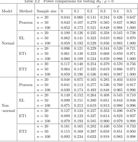
The Monte Carlo power of the level α = 0.05 test statistic was computed by the relative
frequency of rejecting the null hypothesisH0 :ρ= 0. Table 2.2 presents the Monte Carlo power
of the test statistics obtained from three FEL methods for each sample. For ρ= 0, the power
is the size of the test and it converges to α= 0.05 asn gets larger. In the normal sample, the
power of the test based on ET method is higher than that for EL method when n= 100. The
ET1 method shows smaller type-1 error than the ET2 method when the sample size is small. In the non-normal sample, the EL method seems to have better statistical powers than the ET methods. Overall, the three FEL methods show similar performances in most cases, which is consistent with our theory.
2.6 Conclusions
Empirical likelihood method is useful in incorporating the known constraints of parameters and also in combining information from different sources. The functional-form empirical likeli-hood method proposed in this paper provides a unified approach of handling such constraints without using distributional assumptions on the sample observation. FEL methods allow us
to set a more flexible objective function as well as a flexible weight function. Thus, computa-tional efficiency can be achieved by finding a simple weight function in the FEL method. For example, in the simulation study, the computing time for the ET method is much shorter than the computing time for the EL method.
The FEL method can be used to provide a likelihood ratio test with a chi-square limiting distribution. Also, a profile likelihood ratio test can be derived using the orthogonality of the log-likelihood functions. To improve the coverage properties of the FEL in the small sample sizes, some cutting-edge techniques such as bootstrap calibration (Hall and Horowitz, 1996) or the Bartlett correction (Chen and Cui, 2006) can be used. Further investigation in this direction, including the Higher order expansion as in Liu and Chen (2010), is not discussed here and will be a topic of future research.
● ● ● ● ● ● ● ●● ●● ●●● ●●● ●●●●●●●●●●●●●●●●●●●●●●●●●●●●●●●●●●●●●●●●●●●●●●●●●●●●●●●●●●●●●●●●●●●●●●●●●●●●●●●●●●● 0 200 400 600 800 1000 1.005 1.010 1.015 1.020 1.025 muy K emuy ● ● ● ● ● ● ● ● ●● ●● ●●● ●●●●●●●●●●●●●●●●●●●●●●●●●●●●●●●●●●●●●●●●●●●●●●●●●●●●●●●●●●●●●●●●●●●●●●●●●●●●●●●●●●●●● 0 200 400 600 800 1000 0.015 0.020 0.025 0.030 0.035 0.040 0.045 lambda1 K elambda1 ● ●● ● ● ●●●●● ● ●●● ●● ● ● ● ● ● ● ● ●● ● ● ● ● ● ● ● ●● ● ● ● ● ●● ● ●● ● ●● ● ● ●● ● ● ● ● ● ●●● ● ● ● ● ● ● ● ● ● ● ● ● ●● ●● ● ● ● ● ● ● ● ●● ● ●● ● ● ● ●●● ●● ● ●●●● ● 0 200 400 600 800 1000 −4e−08 −2e−08 0e+00 2e−08 4e−08 lambda2 K elambda2
Table 2.1 Monte Carlo relative efficiency of the point estimators.
Model Situation Sample size(n) EL ET1 ET2
S1 n= 20 1.0000 1.0000 1.0000 n= 50 1.0000 1.0000 1.0000 n= 100 1.0000 1.0000 1.0000 S2 n= 20 1.2192 1.2496 1.2375 n= 50 1.2729 1.2782 1.2772 Normal n= 100 1.3184 1.3146 1.3153 S3 n= 20 1.2765 1.3377 1.3267 n= 50 1.3183 1.3364 1.3337 n= 100 1.3295 1.3339 1.3337 S4 n= 20 1.1478 1.2244 1.2262 n= 50 1.2558 1.2721 1.2754 n= 100 1.3022 1.3042 1.3084 S1 n= 20 0.9960 1.0000 1.0000 n= 50 0.9988 1.0000 1.0000 n= 100 1.0000 1.0000 1.0000 S2 n= 20 1.5547 1.7117 1.6455 n= 50 1.5597 1.9005 1.8908 Non-normal n= 100 1.5233 1.9040 1.8990 S3 n= 20 1.0676 1.1901 1.1632 n= 50 1.0875 1.1592 1.1388 n= 100 1.1518 1.2014 1.1839 S4 n= 20 1.2721 1.3700 1.3067 n= 50 1.2966 1.3691 1.3579 n= 100 1.4289 1.5062 1.5188
Table 2.2 Power comparisons for testingH0 :ρ= 0
ρ
Model Method Sample size 0 0.1 0.2 0.3 0.4 0.5
Pearson n= 20 0.044 0.060 0.141 0.244 0.426 0.647 n= 50 0.043 0.107 0.279 0.565 0.837 0.963 n= 100 0.052 0.172 0.521 0.848 0.988 1.000 EL n= 20 0.100 0.126 0.235 0.358 0.545 0.738 n= 50 0.062 0.141 0.323 0.610 0.863 0.970 Normal n= 100 0.059 0.192 0.529 0.856 0.985 1.000 ET1 n= 20 0.096 0.121 0.229 0.344 0.520 0.721 n= 50 0.061 0.138 0.323 0.608 0.859 0.971 n= 100 0.060 0.189 0.534 0.859 0.986 1.000 ET2 n= 20 0.117 0.140 0.254 0.379 0.570 0.756 n= 50 0.064 0.147 0.335 0.619 0.866 0.971 n= 100 0.059 0.196 0.536 0.861 0.987 1.000 Pearson n= 20 0.048 0.075 0.165 0.285 0.403 0.610 n= 50 0.041 0.113 0.277 0.536 0.769 0.917 n= 100 0.039 0.174 0.492 0.848 0.965 0.996 EL n= 20 0.149 0.152 0.264 0.408 0.545 0.710 n= 50 0.099 0.151 0.380 0.651 0.843 0.946 Non n= 100 0.075 0.212 0.619 0.913 0.980 0.996 -normal ET1 n= 20 0.127 0.124 0.227 0.353 0.496 0.678 n= 50 0.089 0.123 0.337 0.614 0.823 0.937 n= 100 0.079 0.193 0.585 0.900 0.979 0.998 ET2 n= 20 0.161 0.165 0.282 0.430 0.558 0.733 n= 50 0.115 0.169 0.397 0.658 0.851 0.950 n= 100 0.092 0.234 0.633 0.918 0.983 0.998
CHAPTER 3. A UNIFIED THEORY ON EMPIRICAL LIKELIHOOD METHODS WITH MISSING DATA AND SURVEY SAMPLING
A paper submitted to theAustralian and New Zealand Journal of Statistics(revision invited)
Sixia Chen and Jae Kwang Kim
Abstract
Efficient estimation with missing data is an important practical problem with many appli-cation areas. Survey sampling can be treated as a missing data problem where the sample is treated as a realization of a known response mechanism. Parameter estimation under nonre-sponse is considered when the parameter is defined as a solution to an estimating equation. Using a response probability model, a complete-response empirical likelihood method can be constructed and the nonparametric maximum likelihood estimator can be obtained by solv-ing the weighted estimatsolv-ing equation where the weights are computed by maximizsolv-ing the complete-response empirical likelihood subject to the constraints that incorporate the auxil-iary information obtained from the full sample. Often the constraints are constructed from the working outcome regression model for the conditional distribution of the estimating func-tion given the observafunc-tion. The proposed method achieves the semi-parametric lower bound when we correctly specify the conditional expectation of the estimating function, regardless of whether the response probability is known or estimated. When the response probability is esti-mated nonparametrically, the resulting empirical likelihood method automatically achieves the semi-parametric lower bound without specifying the conditional distribution of the estimating function. The proposed method is also applicable to two-phase sampling. Asymptotic theories
are derived and simulation studies are also presented.
Key Words: Missing at random; Nonparametric estimation; Response mechanism; Propensity score.
3.1 Introduction
The empirical likelihood (EL) method, proposed by Owen (1988, 1990), has become a very powerful tool for nonparametric inference in statistics. It uses a likelihood-based approach without having to make a parametric distributional assumption about the data observation. Thus, the EL method often leads to efficient estimation and enables likelihood-ratio type in-ference. Qin and Lawless (1994) considered the situation when the parameter of interest is the solution to a system of estimating equations. Owen (2001) provides a comprehensive overview of the EL method.
Under existence of missing data or survey data, however, the EL method is not directly applicable and some adjustment needs to be made. Qin (1993) addressed this problem using a biased sampling argument of Vardi (1985). Wang and Rao (2002) used regression-type imputa-tion approaches to empirical likelihood inference. Wang and Chen (2009) used a nonparametric regression imputation approach to handle missing data in the empirical likelihood inference. The imputation approach uses some assumptions about the missing data given the observed data and usually assumes that the response mechanism is ignorable in the sense of Rubin (1976). Under an ignorable missing mechanism, the explicit modeling of the response model is avoided. In the case of survey sampling, Chen and Sitter (1999) considered the pseudo empirical like-lihood estimator that uses the sampling weight in the empirical log-likelike-lihood function. Kim (2009) considered an alternative empirical likelihood function based on the biased sampling likelihood of Vardi (1985) and Qin (1993). Wu and Rao (2006) discussed interval estimation using the pseudo empirical likelihood. Note that the survey sampling can be treated as a special case of missing data problem, where the sample is obtained by a planned missing mechanism and the first-order sample inclusion probability corresponds to the response probability in the usual missing data problem. The main difference is that the sample inclusion probabilities are
known in survey sampling, as the missing mechanism is planned by the sampling design. In this paper, we consider an alternative approach to handling missing data using a model for response probability. Use of parametric response probability model in the empirical likelihood inference has been considered in Qin and Zhang (2007) and in Chen et al. (2008). Qin et al. (2009) and Tan (2011) considered using EL to model the complete likelihood, where the nonparametric likelihood function is computed for the whole sample including the units with missing data. The use of complete likelihood attains the full efficiency and also provides a nice theory of the limiting chi-square distribution in the likelihood ratio test statistics. However, in some practical case, the unit-level information for the complete likelihood is not always available and the complete likelihood cannot be computed. For example, in survey sampling, the individual values of auxiliary variable in the non-sampled part are not usually available. In this case, the approach of using the complete likelihood for the finite population may not be applicable.
If the response mechanism is nonparametrically modeled, the literature is somewhat sparse. Cheng (1994) discussed some asymptotic properties of the mean estimator using the kernel regression method to estimate the conditional outcome regression model under an ignorable missing case. Recently, Kim and Yu (2011) extended the approach of Cheng (1994) to han-dle nonignorable nonresponse. Xue (2009) discussed an empirical likelihood method for linear models using the weights computed from a nonparametric model where the kernel regression method is used to estimate the response model. Da Silva and Opsomer (2009) considered an-other type of nonparametric response probability estimation using local polynomial regression. Hirano et al (2003) and Cattaneo (2010) discussed semiparametric efficiency of the nonpara-metric response propensity estimators in the context of estimating average treatment effect in econometrics.
In this paper, we propose a unified approach of the EL method with missing data that avoids using the complete likelihood. Under the setup of estimating function in Qin and Law-less (1994), the proposed method can handle the situation regardLaw-less of whether the response probabilities are known or estimated, parametrically or even nonparametrically. When the response probabilities are known, the proposed method can be applied to survey weighting
problems when the first-order inclusion probabilities are known. Incorporating the population level auxiliary information into the weights in the sample is an important problem in survey sampling and is often called calibration weighting. Calibration weighting is considered in
Dev-ille and S¨arndal (1992), Fuller (2002), and Kim and Park (2010), among others. The proposed
method can be directly applicable to the calibration weighting problem.
When the response probabilities are estimated from a parametric model, the proposed method under ignorable response mechanism is similar to the method of Qin and Zhang (2007). The proposed method is directly applicable to the problem of the propensity score weighting method. The propensity score weighting method can be found, for example, in Durrant and Skinner (2006), Kim and Kim (2007), and Chang and Kott (2008). We show that employing EL method using a suitable choice of control variable leads to efficient estimation in the sense that it achieves the lower bound of the asymptotic variance. Optimal choice of the control variable requires correct specification of the conditional distribution of the missing data given the observation. Under the nonparametric propensity score method, which will be discussed in Section 5, the lower bound of the asymptotic variance can be achieved without correctly specifying the conditional distribution.
In Section 2, we first review the existing methods of empirical likelihood under missing data and discuss a unified approach of the EL method. Asymptotic properties of the proposed estimator under known response probabilities are discussed in Section 3. The proposed EL estimator is discussed under estimated response probability in Section 4. Use of the nonpara-metric response model for the EL approach is discussed in Section 5. The proposed method is extended to two-phase sampling in Section 6. Results from two simulation studies are reported in Section 7.
3.2 Basic setup
Consider a multivariate random variable (X, Y) with distribution function F(x, y) which
is completely unspecified except that E{U(X, Y;θ0)} = 0 for some θ0. We are interested in
estimating the parameterθ0 from a random sample of the distribution. To avoid unnecessary
that the dimension of U is equal to the dimension of θ.
If (xi, yi), i= 1,2, . . . , n, aren independent realizations of the random variable (X, Y), a
consistent estimator of θ0 can be obtained by solving
n
X
i=1
U(xi, yi;θ) = 0. (3.1)
In this paper, we consider the problem of estimating θ0 when x is always observed and y is
subject to missingness. Let ri = 1 if yi is observed and ri = 0 otherwise. We consider an
approach based on the empirical likelihood (EL) method. To explain the idea, first note that the joint density of the observed data can be written as
pnr(1−p)n−nr × Y ri=1 f(xi, yi|ri= 1) Y ri=0 f(xi|ri= 0), (3.2)
where nr is the response sample size, p = P r(r = 1), f(x, y|r) is the conditional density of (X, Y) given r, and f(xi|ri = 0) =
R
f(xi, yi|ri = 0)dyi is the marginal density of X among
r= 0.
In the empirical likelihood approach, the distribution is assumed to have the support on the sample observation. Let F1(x, y) = P r(X ≤ x, Y ≤y|r = 1) and F0(x, y) = P r(X ≤ x, Y ≤
y|r = 0). Under the empirical likelihood approach, we can express
F1(x, y) =
X
ri=1
ωiI(xi≤x, yi ≤y), (3.3)
whereP
ri=1ωi= 1, ωi is the point mass assigned to (xi, yi) in the nonparametric distribution of F1(x, y), and I(B) is an indicator function for event B. To express F0(x, y) using ωi, note that we can write
f(xi, yi|ri = 0) =f(xi, yi|ri = 1)× Odd(xi, yi) E{Odd(xi, yi)|ri = 1} , where Odd(x, y) = P r(r= 0|x, y) P r(r= 1|x, y). Thus, we can expressF0(x, y) =P r(X≤x, Y ≤y|r= 0) by
F0(x, y) = P ri=1ωiOiI(xi ≤x, yi ≤y) P ri=1ωiOi , (3.4)
where Oi = Odd(xi, yi). Note that F0(x, y) is completely determined by two factors: ωi and
Oi. The factor ωi is determined by the distribution F1(x, y) and the factor Oi is determined
by the response mechanism. If Odd(x, y) is a known function of (x, y), then we have only to
determineωi.
From (3.4), the joint distribution of (x, y) can be written as
Fw(x, y) = p× X ri=1 ωiI(xi≤x, yi ≤y) + (1−p)× ( P ri=1ωiOiI(xi≤x, yi ≤y) P ri=1ωiOi ) = p× ( X ri=1 ωiI(xi≤x, yi ≤y) + (1/p−1) P ri=1ωiOiI(xi ≤x, yi≤y) P ri=1ωiOi ) .
Note that (3.3) implies
X ri=1 ωi(Oi+ 1) = E 1 π(X, Y)|r= 1 = Z 1 π(x, y)f(x, y|r = 1)dxdy = Z 1 π(x, y) π(x, y)f(x, y) p dxdy= 1/p. Thus, we have P ri=1ωiOi = 1/p−1 and Fw(x, y) = P ri=1ωi(1 +Oi)I(xi≤x, yi ≤y) P ri=1ωi(Oi+ 1) .
We propose maximizing the partial likelihoodQ
ri=1f(xi, yi|ri = 1) in (3.2) in constructing the empirical likelihood. Thus, the proposed empirical likelihood approach can be formulated as maximizing le(θ) = X ri=1 log (ωi), (3.5) subject to X ri=1 ωi = 1, X ri=1 ωi(1 +Oi)U(xi, yi;θ) = 0. (3.6)
Note that, in constraint (3.6), the observed values ofxiwithri = 0 are not used. To incorporate the partial information, we can impose
P ri=1ωi(1 +Oi)h(xi;θ) P ri=1ωi(1 +Oi) =n−1 n X i=1 h(xi;θ). (3.7)
There are several other approaches using the empirical likelihood with missing data. Qin et al. (2002) considered using empirical likelihood for nonignorable nonresponse. Wang and Rao (2002) proposed empirical likelihood-based inference under imputation for missing response data. Qin and Zhang (2007) proposed an empirical likelihood method for estimating the mean response under ignorable missing data where the response probability πi = P r(ri = 1|Xi) is parametrically modeled byπi=πi(φ0) for some φ0.Specifically, they proposed maximizing
l= X ri=1 lognπi( ˆφ)pi/ˆν o , subject to X ri=1 pi= 1, X ri=1 piπi( ˆφ) = ˆν, X ri=1 pih(xi) =n−1 n X i=1 h(xi), (3.8)
where ˆφ is the maximum likelihood estimator of φ0 in the response probability, h(xi) is an
arbitrary variable and ˆν =n−1Pn
i=1πi( ˆφ). Once the estimated probability ˆpi is computed by
the above maximization procedure, the population mean can be estimated by ˆθ=P
ri=1pˆiyi. Chen et al. (2008) built two empirical likelihoods for response and non-response variables separately and formulated two estimating equations based on these two empirical likelihoods. In the context of the current setup, their proposed method can be described as maximizing
l=P ri=1log(pi) + P rj=0log(qj),subject to P ri=1pi= 1, pi ≥0, P rj=0qj = 1, qj ≥0,and X ri=1 pi h(xi;θ)−µ πi( ˆφ) = 0, X rj=0 qj h(xj;θ)−µ 1−πj( ˆφ) = 0, (3.9)
where ˆφ is the maximum likelihood estimator. Qin et al. (2009) considered maximizing the
complete likelihood lc=Pni=1log(ωi) subject to n X i=1 ωi = 1, n X i=1 ωi ri πi Ui(θ) = 0, (3.10) and n X i=1 ωi( ri πi −1)hi(θ) = 0, n X i=1 ωi{ri−πi(φ)} ∂πi(φ)/∂φ πi(φ){1−πi(φ)} = 0. (3.11)
The computation requires that the individual values of xi forri = 0 be available, which is not
always possible, as discussed in Section 1. For example, in survey sampling problem, we only observe (xi, yi) for ri = 1 and the aggregate information ¯xn=n−1
Pn
i=1xi is available. In this case, the method of Qin et al. (2009) is not applicable.
In Section 3, some asymptotic properties of the proposed EL estimator described in (3.5 )-(3.7) are developed for the case whenπi=P r(ri = 1|xi, yi) is a known function of (xi, yi). In particular, we show that the optimal choice of h(xi;θ) that minimizes the asymptotic variance
of the resulting EL estimator of θis
h∗(xi;θ) = ˜U(xi;θ)≡E{U(xi, yi;θ)|xi}.
In Section 4, we consider the case where πi = P r(ri = 1 | xi, yi) is a parametric model
of the form P r(r = 1 |x, y) = π(x;φ0) for some φ0. By plugging estimator ˆφ of φ0 into the
empirical likelihood procedure, we can find the empirical likelihood estimator. The asymptotical
properties of this estimator are discussed in Section 4. If a parametric form of π is unknown,
we can use a nonparametric model forπ. Asymptotical properties of the EL estimator using a
nonparametric estimator of π are discussed in Section 5.
3.3 Estimation with known response probability
In this section, we assume that the true response probability π = P r(r = 1|X, Y) is
known, which is often the case with survey sampling whereπi denotes the first-order inclusion
probability and the response indicator, r, represents the sampling indicator. The regularity
conditions of this section can be found in the section A of Appendix B. Our proposed estimator introduced in Section 2, (3.5)-(3.7), can be described as maximizing
l= X ri=1 log(ωi), (3.12) subject to X ri=1 ωi = 1, X ri=1 ωiπi−1 ( hi(θ)−n−1 n X i=1 hi(θ) ) = 0, X ri=1 ωiπ−1i Ui(θ) = 0. (3.13)
For θ = E(Y), a popular choice of h(θ) is h(θ) = x. In this case, the EL estimator of θ
is obtained by ˆθh1 = Pri=1w∗iπ −1 i yi/ P ri=1w ∗ iπ −1 i where w ∗ i = n−1r {1 + ˆλπ −1 i (xi −x¯n)} −1, ¯
xn=n−1Pni=1xi and ˆλis constructed to satisfy Pri=1w
∗
iπ
−1
i (xi−x¯n) = 0.
The following theorem presents some asymptotic properties of the EL estimator ˆθh1. The
Theorem 3.3.1 Letθˆh1 be the solution to the maximization above. Then, under the regularity
conditions (C1)-(C5) in section A of Appendix B, we have
ˆ θh1−θ0=τ 1 n n X i=1 ri πi Ui(θ0)−B( ri πi −1)˜hi(θ0) +op(n−1/2), (3.14) where˜hi(θ0) =hi(θ0)−µh, µh=E(h), B=E(U˜h0/π) n E(˜h˜h0/π)o−1andτ =− {E(∂U/∂θ)}−1
evaluated at θ=θ0. Hence, we have
√
nθˆh1−θ0
→dN(0, Vh1), (3.15)
where →d denotes convergence in distribution,V
h1 =τΩh1τ0 and Ωh1 =V nr π U−B˜h+Bh˜o=E (1 π −1)(U −B ˜ h)⊗2 +V(U), (3.16) and A⊗2 =AA0.
Because Ωh1 =E{(π−1−1)(U −B˜h)⊗2}+V(U), we always haveV(ˆθh1)≥V(ˆθn),where ˆ
θn is the solution to (3.1). According to the above theorem, we can get the consistent
variance estimator by using ˆVh1 = ˆτΩˆh1τˆ
0 , where ˆτ = −nn−1Pn i=1riπi−1(∂Ui(ˆθh1)/∂θ) o−1 and ˆΩh1 = (n− 1)−1(ηi − η¯)2, where ηi = riπ−1i n Ui(ˆθh1)−Bˆ˜hi(ˆθh1) o + ˆB˜hi(ˆθh1), Bˆ = ˆ E(Uh˜0/π) n ˆ E(˜hh˜0/π) o−1 , ˆ E(U˜h0/π) =n−1 n X i=1 riπi−2Ui(ˆθh1)˜h 0 i(ˆθh1), Eˆ(˜hh˜ 0 /π) =n−1 n X i=1 riπ−2i ˜hi(ˆθh1)˜h 0 i(ˆθh1), with ˜hi(ˆθh1) =hi(ˆθh1)−µˆh and ˆµh=n−1Pni=1hi(ˆθh1).
For the special case ofθ=E(Y) and h=x, after some algebra, we have
ˆ θh1 = ˆy¯d−Bˆ1Bˆ−12 (ˆx¯d−x¯n) +op(n−1/2), where (ˆy¯d,xˆ¯d) = ( P ri=1π −1 i ) −1(P ri=1π −1 i yi, P ri=1π −1 i xi),Bˆ1 =n−1 P ri=1π −2 i (xi−xˆ¯d)(yi− ˆ ¯
yd) and ˆB2 = n−1Pri=1πi−2(xi −xˆ¯d)2, which is close to the optimal estimator within the linear class. The resulting estimator is asymptotically equivalent to the optimal EL estimator considered in Kim (2009).
Remark 3.3.1 The EL estimator of Chen et al. (2008) satisfies √ n(ˆθc−θ0)→dN(0, Vc), where Vc =τΩhcτ0, Ωhc = V ( r πU−B ∗(r−π)˜h π(1−π) ) , where B∗ = E(U˜h0/π)hEn˜hh˜0/(π(1−π))oi −1
. Thus, the estimator of Chen et al. (2008)
achieves the minimum variance when h/(1−π) ∝ E(U |x) while the asymptotic variance of
the proposed EL estimator is minimized when h ∝ E(U | x). The Qin-Zhang-Leung (QZL)
estimator θˆQZL defined in (3.10) and (3.11) satisfies
√ n(ˆθhq−θ0)→dN(0, Vq), where Vq=τΩhqτ0, Ωhq = V r πU − r−π π Bqh ,
andBq=E{(π−1−1)U h0}[E{(π−1−1)hh0}]−1.Note that the choice of B=Bq minimizes the
variance of(r/π)U−((r−π)/π)Bhand the QZL estimator is optimal in the sense that it
mini-mizes the variance among its class. This is because QZL estimator uses the complete likelihood
Pn
i=1log(ωi) while our proposed estimator uses only partial likelihood. If h ∝ E(U|X), then
all the estimators, excluding the estimator of Chen et al. (2008), achieve the same asymptotic variance. A numerical comparison is also made through a simulation study in Section 6.
In the following corollary, we find an optimal constraint that minimizes the asymptotic
variance in (3.15). The proof is presented in section C of Appendix B.
Corollary 3.3.1 Under the setup of Theorem 3.3.1, the asymptotic variance of θˆh1 is
mini-mized when h∝h∗ =E(U|X).The asymptotic variance satisfies
Vh1 ≥τ ( E U U 0 π ! −E 1−π π h ∗U0 ) τ0. (3.17)
The lower bound in (3.17) is the same as the semi-parametric lower bound for the asymptotic
Remark 3.3.2 To compute the solution to the constrained optimization problem of maximizing
(3.12) subject to (3.13), the following two-step algorithm can be used. In the first step, the
opti-mal weight that maximizes (3.12) subject toP
ri=1ωi = 1and P ri=1ωiπ −1 i {ˆhi−n−1 Pn j=1hˆj}=
0 are computed, whereˆhi =hi(ˆθ0) andθˆ0 is the solution toPri=1π−1i Ui(θ) = 0. In the second
step, we can get the resulting EL estimator θˆh1 by solving
N X i=1 ˆ ωi Ii πi Ui(θ) = 0.
Such two-step algorithm was discussed in Chaudhuri, Handcock and Rendall (2008) when the
control function hi does not depend on θ. Using ˆhi = h(xi; ˆθ), where θˆ is any
√
n-consistent
estimator ofθ, in the two-step optimization is asymptotically equivalent to the original solution.
3.4 Estimation with unknown response probability
We now consider the case when the response probability is known up to some parameter and has the known form
P r(r = 1|X, Y) =π(X;φ0),
for some φ0.Thus, we assume that the response mechanism is ignorable. We also assume that
there exists ˆφsuch that ˆ φ−φ0= 1 n n X i=1 b(xi, ri;φ0) +op(n−1/2), (3.18)
for some functionbwithE{b(Xi, ri;φ0)}= 0 andV ar{b(Xi, ri;φ0)}=Vb,whereVb is positive definite.
If the true response probability πi =πi(φ0) is estimated by ˆπi =πi( ˆφ), then the proposed
EL estimator can be described as maximizing (3.12) subject to
X ri=1 ωi = 1, X ri=1 ωiπˆi−1 ( hi(θ)−n−1 n X i=1 hi(θ) ) = 0, (3.19) and X ri=1 ωiπˆ−1i U(θ;xi, yi) = 0. (3.20)
Theorem 3.4.1 Let φˆ be a √n-consistent estimator of φ0, satisfying (3.18). Let θˆh2 be
ob-tained by maximizing (3.12) subject to the constraints (3.19) and (3.20). Under the same
regularity conditions as Theorem 3.3.1 and (3.18), we have
ˆ θh2−θ0=τ 1 n n X i=1 ri πi Ui(θ0)−B( ri πi −1)˜hi(θ0)−Cbi(φ0) +op(n−1/2), (3.21)
where B is defined in (3.14), τ = − {E(∂U/∂θ)}, C = E
n
π−1(U−B˜h)(∂π/∂φ)0
o and
bi(φ0) =b(xi, ri;φ0) defined in (3.18). Hence, we have
√ n(ˆθh2−θ0)→dN(0, Vh2), where Vh2 =τΩh2τ 0 ,and Ωh2 =V n rπ−1(U −Bh˜) +Bh˜−Cbo.
A consistent variance estimator of Vh2 can be constructed by
ˆ Vh2 = ˆτΩˆh2τˆ 0 ,where ˆτ =−nn−1Pn i=1riπˆ−1i (∂Ui(ˆθh2)/∂θ) o−1 and ˆΩh2 = (n−1)−1 Pn i=1(ηi− ¯ η)2,whereηi=riπˆi−1 n Ui(ˆθh2)−Bˆ˜hi(ˆθh2) o + ˆB˜hi(ˆθh2)−Cbˆ i( ˆφ), ˆ C=n−1 n X i=1 riπˆi−2 n Ui(ˆθh2)−Bˆ˜hi(ˆθh2) o (∂πˆi/∂φ)T, Bˆ = ˆE(U h 0 /π) n ˆ E(˜h˜h0/π) o−1 , where ˆE(Uh˜0/π) = n−1Pn i=1riπˆi−2Ui(ˆθh2)˜h 0 i(ˆθh2) ,Eˆ(˜hh˜ 0 /π) =n−1Pn i=1riπˆi−2˜hi(ˆθh2)˜h 0 i(ˆθh2), with ˜hi(ˆθh2) =hi(ˆθh2)−µˆh and ˆµh=n−1Pni=1hi(ˆθh2).
Comparing (3.21) with (3.14), we have an extra term,−Cbi(φ0), in the linearization. This
is because we have additional randomness due to estimating parameter φ0.
Remark 3.4.1 If we use h = ah∗ = aE(U|X) in the constraint (3.19) for some constant
a6= 0, we haveB =E(U h0/π)E−1(hh0/π) =a−1I and
C=Eπ−1(U−Bh)(∂π/∂φ)0 =EEπ−1(U −h∗)(∂π/∂φ)0|X = 0.
Thus, the asymptotic variance is equal to Vh2=τ E U U0 π −E 1−π π h ∗U0 τ0,
which is equal to the lower bound in (3.17) when the propensity score is known. Under the
optimal choice of h, the lower bound for the asymptotic variance is achieved regardless of
According to Remark 3.4.1, the choice of ˆφdoes not make any difference in the asymptotic variance of ˆθh2, as long as h ∝ E(U |X) is used in (3.19). If h ∝E(U | X) does not hold,
then the choice of ˆφ makes a difference. While the MLE ofφ0 is a popular choice, it does not
necessarily lead to the optimal estimator. To see this, let ˆφq be a consistent estimator of φ0
that can be obtained by solving the following equation: 1 n n X i=1 ri πi(φ) −1 qi(φ) = 0, (3.22)
whereqi(φ) is an arbitrary function to make the solution of (3.22) unique. Note that equation
(3.22) can be called the calibration equation in the sense that the estimator for the mean of
qi using the propensity score is equal to the sample mean of qi. The MLE of φ0 also belongs
to the class because it satisfies (3.22) withqi =πilogit(πi). Under some regularity conditions, we have ˆφq→pφ0,regardless of the choice of qi. However, the efficiency can be different for a different choice ofqi. The following theorem discusses the optimal choice ofq in the calibration equation (3.22).
Theorem 3.4.2 Letφˆq be the estimator which solves (3.22) and satisfiesφˆq →p φ0.Under the
same regularity conditions as Theorem 3.4.1, we have
ˆ θh2−θ0 =τ 1 n n X i=1 ri πi Ui(θ0)−( ri πi −1) n B˜hi(θ0) +CS−1q(φ0) o +op(n−1/2), (3.23)
whereBis defined in (3.14),τ =− {E(∂U/∂θ)}, S =Enπ−1q(∂π/∂φ)0o, C =Enπ−1(U −B˜h)(∂π/∂φ)0o.
Hence, we have √ n(ˆθh2−θ0)→dN(0, Vh2), where Vh2=τΩh2τ 0 ,andΩh2 =V n rπ−1U −(rπ−1−1)(B˜h+CS−1q)o.In addition, we have Vh2 ≥τ V rπ−1U −(rπ−1−1)h∗ τ0
with equality if α0q=h∗−B˜h for some α.
In Theorem 3.4.2, the meaning ofh∗−B˜his the residual for the regression ofh∗=E(U|X) on ˜h. If h∝h∗, then the residual is equal to zero and the lower bound is achieved, as discussed
can be improved by how wellq explains the conditional expectationE(U |X). In the extreme case ofh≡0, the choice ofq ∝h∗ achieves the lower bound while the choice ofqi ∝πih∗, which
corresponds to the maximum likelihood estimation ofφ0, does not achieve the lower bound and
thus leads to less efficient estimation.
3.5 Nonparametric estimation of the response mechanism
In this section, we consider nonparametric estimation of the response probability. For
simplicity, we assume the response mechanism is ignorable,π(x) =P r(r = 1|x),and consider
estimation ofπ nonparametrically. To this end, we consider kernel estimation of the response
model as below: ˆ πH(x) = Pn i=1KH(x−Xi)ri Pn j=1KH(x−Xj) , (3.24)
where KH(s) is the kernel function which satisfies certain regularity conditions and H is the
bandwidth. In addition, we defineKH(s, t) =K((s−t)/H).Letf(x) be the probability density
function of X. In addition to regularity conditions (C1)-(C5) in the section A of Appendix B,
we also assume the following regularity conditions:
(C6)f(x) andπ(x) have bounded partial derivatives with respect tox up to an order q with
q≥2,2q > dx almost surely, wheredx is the dimension ofx.
(C7) The kernel functionK(s) is a probability density function such that
1. It is bounded and has compact support. 2. R
K(s1, . . . , sdx)ds1. . . dsdx = 1,
3. R sliK(s1, . . . , sdx)ds1. . . dsdx = 0 for any i= 1, . . . , dx and 1≤l < q. 4. R
sqiK(s1, . . . , sdx)ds1. . . dsdx 6= 0.
(C8)nH2dx → ∞, √nHq→0,asn→ ∞.
(C9) 1> π(x)> d >0 almost surely.
Conditions (C6)-(C8) are common conditions used for nonparametric problems. In
is used to produce consistent estimation of the conditional distribution as well as control the convergence rate of response probability estimation. Condition (C9) is used to avoid extreme propensity scores.
Under those regularity conditions, the proposed empirical likelihood method can be con-structed similarly by maximizing (3.12) subject to
X ri=1 ωi= 1, X ri=1 ωiπˆ−1i,H hi(θ)−n−1 n X i=1 hi(θ) = 0, X ri=1 ωiˆπ−1i,HUi(θ) = 0, (3.25) where ˆπi,H = ˆπH(xi).
The following theorem presents some asymptotic properties of the proposed EL estimator of θ0 using nonparametric response probability (3.24).
Theorem 3.5.1 Let θˆh3 be the empirical likelihood estimator that is obtained by maximizing
(3.12) subject to (3.25). Under the regularity conditions (C1)-(C9), we have
ˆ θh3−θ0 = −τ 1 n n X i=1 ri πi Ui(θ0)− 1 n n X i=1 (ri πi −1)h∗i(θ0) +op(n−1/2), (3.26)
where h∗(θ0) = E{U(θ0)|X} and τ =− {E(∂U/∂θ)}−1 evaluated at θ =θ0. Furthermore, we
have √ n(ˆθh3−θ0)→dN(0, Vh3), where Vh3 =τΩh3τ 0 and Ωh3=V rπ−1(U −h∗) +h∗ .
By Theorem 3.5.1, the asymptotic variance of ˆθh3 using nonparametric ˆπi,H is equal to the
semiparametric lower bound in (3.17). Note that the linearization in (3.26) does not depend on
the choice of h in (3.25). This means that the same result (3.26) can be achieved for different
choices of h. This is because, according to (F.9) in the proof of Theorem 3.5.1 in Section F of
Appendix B, we have 1 n n X i=1 ri ˆ πi,H ˜ hi− 1 n n X i=1 ˜ hi =op(n−1/2),
where ˜h=h−µh and his any arbitrary function ofx with some moment conditions described
in section A of Appendix B. In addition, the second constraint in (3.25) can be written as
P
ri=1ωiπˆ
−1
i,H(˜hi−n
−1Pn