Segmentation and classification of lung nodules from Thoracic CT scans : methods based on dictionary learning and deep convolutional neural networks.

(1)

University of Louisville University of Louisville

ThinkIR: The University of Louisville's Institutional Repository

Electronic Theses and Dissertations

5-2019

Segmentation and classification of lung nodules from Thoracic

CT scans : methods based on dictionary learning and deep

convolutional neural networks.

Mohammad Mehdi Farhangi University of Louisville

Follow this and additional works at: https://ir.library.louisville.edu/etd

Part of the Computer Engineering Commons

Recommended Citation Recommended Citation

Farhangi, Mohammad Mehdi, "Segmentation and classification of lung nodules from Thoracic CT scans : methods based on dictionary learning and deep convolutional neural networks." (2019). Electronic Theses and Dissertations. Paper 3301.

(2)

SEGMENTATION AND CLASSIFICATION OF LUNG NODULES FROM THORACIC CT SCANS: METHODS BASED ON DICTIONARY LEARNING

AND DEEP CONVOLUTIONAL NEURAL NETWORKS

By

Mohammad Mehdi Farhangi

A Dissertation

Submitted to the Faculty of the

J.B. Speed School of Engineering of the University of Louisville

in Partial Fulfillment of the Requirements for the Degree of

Doctor of Philosophy

in Computer Science and Engineering

Department of Computer Engineering and Computer Science

University of Louisville Louisville, Kentucky

(3)

(4)

(5)

AND DEEP CONVOLUTIONAL NEURAL NETWORKS

By

Mohammad Mehdi Farhangi

Dissertation approved on

April 23, 2019

by the following dissertation Committee:

Dissertation Adviser Dr. Amir A. Amini

Dissertation Co-adviser Dr. Hichem Frigui

Dr. Juw Won Park

(6)

ACKNOWLEDGMENTS

Firstly, I would like to express my sincere gratitude to my primary advisor Dr. Amir A. Amini and co-advisor Dr. Hichem Frigui, for their insightful guidance, motivation, and immense knowledge. They have always been patient and supportive in overcoming obstacles I have been facing through my research and writing of this thesis.

I also would like to thank Dr. Albert Seow and his team for analyzing the NLST data; without their help this would not have been possible. I would also like to express my thanks to members of my committee: Dr. Juw Won Park, Dr. Nihat Altiparmak, and Dr. Neal Dunlap for their valuable time and feedback on my thesis. I am also grateful to Dr. Adel Elmaghraby, Chair of CECS Department, who was always supportive during my entire graduate studies.

Last, I should express my gratitude to all other Medical Imaging Lab members at the University of Louisville for their support and for their friendship. I am especially thankful to Benjamin Veasey who developed the software for perparing and pre-processing NLST data and Jungwon Cha who collaborated and helped in different parts of my research.

(7)

ABSTRACT

AND DEEP CONVOLUTIONAL NEURAL NETWORKS Mohammad Mehdi Farhangi

April 23, 2019

Lung cancer is a leading cause of cancer death in the world. Key to survival of pa-tients is early diagnosis. Studies have demonstrated that screening high risk papa-tients with Low-dose Computed Tomography (CT) is invaluable for reducing morbidity and mortality. Computer Aided Diagnosis (CADx) systems can assist radiologists and care providers in reading and analyzing lung CT images to segment, classify, and keep track of nodules for signs of cancer.

In this thesis, we propose a CADx system for this purpose. To predict lung nodule malignancy, we propose a new deep learning framework that combines Convolutional Neural Networks (CNN) and Recurrent Neural Networks (RNN) to learn best in-plane and inter-slice visual features for diagnostic nodule classification. Since a nodule’s volumetric growth and shape variation over a period of time may reveal information regarding the malignancy of nodule, separately, a dictionary learning based approach is proposed to segment the nodule’s shape at two time points from two scans, one year apart. The output of a CNN classifier trained to learn visual appearance of malignant nodules is then combined with the derived measures of shape change and volumetric growth in assigning a probability of malignancy to the nodule.

Due to the limited number of available CT scans of benign and malignant nod-ules in the image database from the National Lung Screening Trial (NLST), we chose to initially train a deep neural network on the larger LUNA16 Challenge database which was built for the purpose of eliminating false positives from detected nodules in thoracic CT scans. Discriminative features that were learned in this application were transferred to predict malignancy. The algorithm for segmenting nodule shapes

(8)

algorithm captures a sparse representation of a shape in input data through a linear span of previously delineated shapes in a training repository. The model updates shape prior over level set iterations and captures variabilities in shapes by a sparse combination of the training data. The level set evolution is therefore driven by a data term as well as a term capturing valid prior shapes. During evolution, the shape prior influence is adjusted based on shape reconstruction, with the assigned weight deter-mined from the degree of sparsity of the representation. The discriminative nature of sparse representation, affords us the opportunity to compare nodules’ variations in consecutive time points and to predict malignancy. Experimental validations of the proposed segmentation algorithm have been demonstrated on 542 3-D lung nod-ule data from the LIDC-IDRI database which includes radiologist delineated nodnod-ule boundaries.

The effectiveness of the proposed deep learning and dictionary learning archi-tectures for malignancy prediction have been demonstrated on CT data from 370 biopsied subjects collected from the NLST database. Each subject in this database had at least two serial CT scans at two separate time points one year apart. The proposed RNN CAD system achieved an ROC Area Under the Curve (AUC) of 0.87, when validated on CT data from nodules at second sequential time point and 0.83 based on dictionary learning method; however, when nodule shape change and appearance were combined, the classifier performance improved to AUC=0.89.

(9)

TABLE OF CONTENTS

Acknowledgments . . . iii

Abstract . . . iv

List of Tables . . . viii

List of Figures . . . ix INTRODUCTION . . . 1 Motivation . . . 1 Lung Anatomy . . . 2 Segmentation . . . 2 Nodule Detection . . . 3 Thesis Objectives . . . 4 Thesis Organization . . . 5

LITERATURE REVIEW ON LUNG NODULE SEGMENTATION . . . 7

Literature Review on Lung Nodule Segmentation . . . 7

Active Shape Models . . . 13

Sparse Shape Composition . . . 15

SCOTS: SPARSE LINEAR COMBINATION OF TRAINING SHAPES . . . . 16

Level Set Segmentation . . . 17

Shape Prior Modeling . . . 20

Shape prior weighting . . . 22

Segmentation algorithm . . . 25

Convergence and Complexity . . . 30

SEGMENTATION RESULTS . . . 31

Dataset . . . 31

(10)

Parameters Settings . . . 33

Results . . . 34

DEEP LEARNING IN MEDICAL IMAGE ANALYSIS . . . 45

Deep Learning . . . 46

Deep Learning for Detection . . . 48

Deep learning for segmentation . . . 49

Deep Learning for Computer-Aided Diagnosis . . . 50

LUNG NODULE MALIGNANCY PREDICTION BASED ON SINGLE TIME POINT AND SEQUENTIAL TIME POINT CT SCANS . . . 52

Recurrent convolutional networks to detect lung nodules based on single time point CT scans . . . 55

Use of shape, and volume growth in two consecutive CT Scans . . . 61

EXPERIMENTAL RESULTS FOR MALIGNANCY PREDICTION FROM NLST DATA SETS . . . 64

Datasets . . . 64

Performance Metrics for Single and Consecutive CT Scan Classifiers . . . . 65

CONCLUSIONS AND FUTURE WORK . . . 76

REFERENCES . . . 79

Appendix A: Commonly Used Acronyms . . . 91

(11)

LIST OF TABLES

1 The algorithm parameters values used for all experiments . . . 34 2 Numerical validation of the algorithm on LIDC-IDRI database . . . 38 3 Inter-observer variability among four radiologists . . . 41 4 Numerical validation of the algorithm, using STAPLE as the ground truth 41 5 Performance of SCoTS on specific nodule types. . . 42 6 Comparison with state of the art algorithms . . . 43

(12)

LIST OF FIGURES

1 Anatomy of Lung . . . 3

2 Classification of lung nodules based on attachment . . . 8

3 Variety of nodule shapes . . . 12

4 Landmark based shape representation . . . 13

5 Representing a nodule shape by SDF . . . 19

6 Encoding two shapes by nodule dictionary . . . 23

7 Shape prior weighting function . . . 25

8 Level set evolution update . . . 28

9 Surface evolution in segmentation process . . . 35

10 Evolution of sparse representation and energy . . . 37

11 Result of the algorithm on samples of the dataset . . . 39

12 Result of segmentation using different dictionaries . . . 40

13 Perceptron . . . 45

14 Annotation variability among readers . . . 53

15 Transfer learning for malignancy prediction . . . 54

16 Architecture of the proposed deep learning . . . 57

17 Diagram of recurrent units . . . 59

18 Malignancy prediction from two time points . . . 63

19 Nodule changes in two time points . . . 66

20 Segmentation Results on NLST database . . . 67

21 Performace on first time point . . . 70

22 Performance on second time point . . . 71

23 performance based on two time points . . . 72

24 Prediction correlation . . . 73

25 prediction correlation . . . 74

(13)

CHAPTER I

INTRODUCTION

1 Motivation

Fatality caused by lung cancer has significant proportions; it is estimated that world-wide 1.1 million people die of lung cancer each year [65]. One reason is because lung cancer is not diagnosed in its early stages; indeed in most cases it is diagnosed after it has already spread through the body. Unfortunately, treatments are not very successful at that point. Screening high risk patients with low-dose Computed Tomography (CT) has shown significant reduction of lung cancer mortality rate [61]. The goal of CT screening is to detect cancer in early stages when there are more options to treat the patient.

As a consequence of the benefits provided by low-dose CT imaging, it is be-ing implemented in large scale in the US. However, this extensive usage results in significant increase of reading efforts for the radiologists. Radiologists mostly read and investigate volumetric CT scans to detect small abnormal lesions including pul-monary nodules. Pulpul-monary nodules are radiologically visible small structures that are roughly spherical [87]. It turns out that these small structured lesions are crucial indicators of lung cancer, and through their size, appearance, and shape of great use for cancer malignancy diagnosis [56]. Based on detected nodules, radiologists and

(14)

surgeons can measure the size and characteristics of nodule, , perform biopsies, and surgical intervention in necessary cases to improve the survival rate.

2 Lung Anatomy

Lungs are a pair of spongy organs located on both side of the chest. When inter-preting the lung CT scans, it is important to have a solid understanding of lung structure. A brief overview of lung anatomy is presented here. Lungs are covered by a tissue layer called pleural, a thin layer of fluid plays as lubricant helping the lung to move smoothly over the exhalation and inhalation.

Each lung can be divided into lobes as shown in Figure 1. Each lobe contains its own separate vascular and lymphatic networks. The right lung is larger because heart is accommodated in the left lung. The left lung divides into upper and lower lobe with a horizontal fissure. The right lung on the other hand, has two fissures which results in three lobes (upper, middle, and lower) lobes.

3 Segmentation

Segmentation is a fundamental step of most CAD systems. By segmenting the nod-ule, the shape characteristics can be extracted, helping the radiologists analyze the malignancy as malignant nodules are more speculated. It also provides information on nodule growth over a period of time. However, segmentation is a challenging prob-lem in lung CT due to the confounding factor that nodules can be attached to the pleural surface with the same Hounsfield Units (HU) or they might have significant overlap with neighboring vessels. From this point of view, Kostis et al. [46] divided

(15)

Figure 1. Anatomy of Lung [2].

lung nodules into four different categories named well-circumscribed, juxta-vascular, juxta-pleural, and pleural tail nodules. The last three cases cause difficulties for density based segmentation algorithms because for these cases the nodules have HU very similar to those in the vascular and pleural space.

4 Nodule Detection

To diagnose lung cancer, it is important to detect and interpret the lung nodules. Fortunately, Low dose CT affords a significant improvement to lung nodule detec-tion in patients in comparison to chest X-ray so that 20% reducdetec-tion in mortality is achieved with low-dose CT scans [61, 62]. However, false positives remains high

(16)

with this modality and a post processing step is needed to reduce false positives. A nodule detector system typically consists of two steps: 1) candidate detection and 2) false positive reduction.

In candidate detection, a large number of candidates are extracted from the whole volumetric lung CT. The aim of this step to include all the nodules in the large set of candidates using a variety of characteristics like intensity, shape features, morphology, etc. This step detect nodules with a very high sensitivity without forcing the system to keep the false positives at a low rate. Reducing the number of false positives is typically carried out in the second stage where an effective classifier in conjunction with discriminative features serve to remove false positives and provide the output with a high sensitivity at a low false positive per scan.

5 Thesis Objectives

The need to go through large number of high resolution CT scans with many slices makes the reading and interpretation of images an arduous task - a tedious process for radiologists. Computer-Aided Detection (CAD) systems have come to assist the radiologists in the reading and interpretation by detecting, segmenting, and keeping track of nodule changes in CT scans and making the process more efficient.

The main objective of this thesis is to develop a CAD system to segment and classify lung nodules in lung CT scans. For nodule segmentation, a general framework is presented which considers shape variability of nodules and brings this information into the segmentation process. We capture the best shape by approximating the evolving surface of a level set model through a linear combination of training shapes

(17)

in a subspace, resulting in a sparse representation of nodule shapes. Sparse encoding provides a tool to validate the shape approximation and force the shape from growing once it reaches the boundary of the nodule.

In nodule classification, we propose to classify nodules as benign and malignant from single time point CT scans, from a pair of consecutive scans, and from a com-bination of the two. With the remarkable successes of convolutional neural networks (CNNs) in computer vision [47, 67], and medical imaging [52], for nodule classifi-cation from single time point scans, we represent nodules with high level features learned from training samples by using a deep convolutional neural network. Deep learning approaches afford us to automatically extract the optimal features for the application of lung nodule classification without the need to investigate and extract hand crafted features. A patch surrounding the nodule is separated and multiple layers including convolutional and max pooling layers are applied to the patches to both find and extract the best features to distinguish between benign and malig-nant nodules. When considering a pair of CT scans acquired over for example a one year period, we would like to determine a quantitative metric of similarity of the two shapes. To this end we represent both nodule through a sparse representation of nodule shapes in two time points and propose a similarity metric from which a malignancy score is derived.

6 Thesis Organization

The thesis is organized in the following order:

(18)

• Chapter II reviews the literature on lung nodule segmentation of CAD systems.

• Chapter III illustrates the proposed method for lung nodule segmentation.

• Chapter IV presents experimental results and evaluation of segmentation on a public database.

• Chapter V reviews the literature on deep learning and its application in medical imaging.

• Chapter VI presents details of our method for malignancy prediction from sequential CT scans.

• Chapter VII reports the experimental results of malignancy prediction evalu-ated on the NLST database.

(19)

CHAPTER II

LITERATURE REVIEW ON LUNG NODULE SEGMENTATION

1 Literature Review on Lung Nodule Segmentation

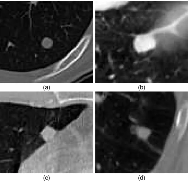
Segmentation of nodules is a fundamental step in every CAD system designed to detect lung cancer. Several attempts have been made to automatically segment nodule boundaries from X-ray computed tomography (CT) scans. But, segmentation is challenging. The challenges mostly come from low contrast and noise. Further confounding the task is that nodules can have a variety of shapes and may be attached to the pleural surface with the same Hounsfield Unit (HU). They may also have significant connections to neighboring vessels. From this point of view, Kostis et al. [46] divided lung nodules into four different categories named well-circumscribed, juxta-vascular, juxta-pleural, and pleural tail nodules. The last three cases pose difficulties for intensity based segmentation algorithms because nodules have HU very similar to those in the vascular and pleural space. Examples of these four categories are shown in Figure 2. In the literature, the challenges have been addressed utilizing shape prior information and refinement [68, 60, 31, 95, 22, 101, 97]. The purpose of shape refinement being to keep the segmented area similar to expected shapes of nodules that are available.

(20)

(a)

(b)

(c)

(d)

Figure 2. Classification of lung nodules based on attachment. (a): Well-circumscribed, (b): Juxta-vascular, (c): Juxta-pleural, (d): Pleural tail

(21)

To deal with nodules having different shape and HU characteristics, previously proposed methods restrict the segmentation to specific nodule types since shape refinement can then be done more accurately [59]. For example, [46, 25] proposed to segment only small solid nodules with homogeneous and solid texture whereas authors in [11] proposed an algorithm to deal with juxta-vascular nodules. In [58], the authors restricted the method to juxta-pleural nodules and in [49], a method was proposed to segment non-solid and part-solid nodules from the rest of the CT scan. In addition, some studies proposed preprocessing and post processing techniques to exclude vessels and the pleural surface from the final segmentation result; in [48], the authors proposed to perform a rough segmentation of juxta-pleural nodules, in-cluding the pleural surface in the segmented result. Considering the fact that lungs are mostly convex except for the diaphragm and the cardiac region, the only cavity in the rough segmentation is separated using convex hull operation as the nodule bound-ary. Threshold-based region growing approach was followed by two post processing steps in [49] to detach pleural surface and vessels from non-solid and part-solid nod-ules. In [5], a multilevel approach consisting of Otsu thresholding, region growing, fuzzy connectivity analysis, morphological operations, and thickening was proposed to segment various types of pulmonary nodules. In [8], another multilevel approach was proposed where segmentation was applied to each nodule slices individually. The authors modeled nodules change in consecutive slices by motion estimation assuming the differences between nodule in slices are small. They subtracted lesion slice from background slice followed by Otsu thresholding and morphological operations to de-tach connected organs. Finally, to segment juxta-vascular nodules, [59] extracted the

(22)

vessels from an initial segmentation by taking advantage of anatomical information where vessels occupy a narrow region of the volume. By defining a threshold on the percentage of segmented voxels in a fixed cubic size, vessels were separated from the nodule.

Reeves, et al. [68] utilized adaptive thresholding, in which the threshold is com-puted separately for each scan to compensate for the variations between two consec-utive scans. The midpoint of the nodule and parenchyma’s density was chosen as the threshold. They applied geometrical constraints to keep the segmented nodule in a spherical shape while removing vessels from the final segmentation. Dehmeshki, et al. [22] proposed sphericity contrast based region growing, in which each pixel of the boundary was added to the segmented region according to their intensity contrast and distance to the center of the region. While the latter metric followed the spheri-cal shape assumption, another shape constraint was applied to stop the segmentation if the size was greater than a predefined threshold. In [91], region growing was also used where the decision of neighbors to be included in the nodule area was carried out by machine learning methods. For each voxel, a feature vector was extracted and fed to a classifier to predict its label based on a linear or non-linear classifier trained over pre-segmented nodules.

Way,et al. [95] proposed to segment 3D lung nodules by a snake based algorithm [43]. They extended gradient, energy and curvature to 3D images, and defined a prior mask energy which penalized the curves that grow beyond the pleural surface. In another attempt to incorporate active contours in this application, Farag, et al. [31] proposed a 2D variational approach to model density of nodules as nonparametric

(23)

Gaussian distributions favoring elliptical shapes. Graph-cut based segmentation is another successful approach to segment nodules in the lung. Ye,et al. [101] used den-sity, shape and spatial features to define an energy function for segmentation. The graph cut algorithm was applied to the over-segmented image previously obtained from unsupervised clustering of image features forcing a spherical shape prior. An-other attempt in this area was by Cha, et al. [97] where a sequence of graph-cuts iterations were performed, each of which with different unary potentials computed from both intensity values and a shape prior. Shape prior in each iteration changes to adapt to the segmented volume in the current iteration.

As it can be seen, many of the previously proposed methods assume that the nodule has spherical or ellipsoidal shape that might be attached to vessel or pleura with similar densities. However, as may be seen in Fig. 3, this assumption is un-realistic in general as the nodules can have complicated structures. The ellipsoidal shape assumption is a limitation, resulting in the segmented surface to become overly rounded, preventing capture of fine structures.

There are methods to incorporate shape prior without restricting the shape to predefined ellipsoid or rounded shapes. In the next section we explore these methods which mostly rely on a training sets consisting of shapes that resemble the segmenting target object. Two of the frequently used methods in this area are Active Shape Model (ASM) [19] and Sparse Shape Composition (SSC) [104].

(24)

(25)

Figure 4. Encoding nodule shapes by landmarks. Taken from [30].

2 Active Shape Models

Active shape models are popular methods in medical image processing to incorporate shape information into anatomical segmentation of objects from Magnetic Resonance (MR) brain images [29, 92], lung CT [92, 96], and liver CT [96]. In its classical form, ASM finds object boundaries using Principal Component Analysis (PCA) with boundary of training shapes given as a set of landmark coordinates. Shapes are represented by a set of landmarks delineating the boundary of the object. An example can be seen in Figure 4. Coordinates of the landmarks are vectorized and stored in a 1-D matrix. The training set is then comprised of all the landmark coordinates stored in this format. ASM then extracts statistical information from the training set. Mean vector shows the average of landmarks in 2-D space, and eigenvectors computed from PCA analysis shows the direction of significant change in the training set. Having mean vector and most significant eigenvectors the direction of variations are computed and any segmented region can then be refined using these information. Refining shapes using ASM has found many applications in segmentation algo-rithms. As some examples, in [12] an iterative graph-cut approach was proposed

(26)

where the initial segmentation provided by graph-cut is refined using extracted sta-tistical information by ASM. The authors validated the feasibility of applying their method to segmenting organ in 3-D CT and MR images.

Other variations of ASM have also been used in graph-cut segmentation frame-work. For example, Grosgeorge et al. [37] used ASM analysis to extract shape information and refine a rough segmented area that was generated by graph-cut seg-mentation. Shapes in their approach have been represented by the Signed Distance Functions (SDF) rather than landmarks. They managed to accurately segment the right ventricle (RV) in MR images and overcome the challenges with low contrast images and tissues attached to the organ. Cha et al. [97, 96, 9] also utilized ASM analysis to iteratively refine the segmented shapes of lung, liver, and lung nodules that outlined using signed distance function.

Another framework which the active shape model has found success in level set based segmentation. In [50] principal component analysis was performed on a set of signed distance functions (SDF) and increased the accuracy of geodesic active contour [6] in segmenting the corpus callusom from MR images. Delineating shapes by SDF, which is considered as an implicit representation, has advantages over ex-plicit ones like landmark based representation [20]. For example, landmark based representations do not permit topological changes of the evolving boundary because this representation is restricted to the labeling of space and making the splitting and merging of curves very complicated if not impossible. In addition, landmark based representations cannot be extended to 3-D space in a straightforward manner and require tedious human effort to find the correspondences between the landmarks in

(27)

training shapes. With the same shape representation, Tsai et al. [89] added scale, rotation and transition to the parameter of curve representation. They tested the method on segmenting left ventricle from cardiac MR images as well as prostate segmentation.

3 Sparse Shape Composition

Another approach proposed by Zhang et al. [104], represents new shapes by a sparse combination of training shapes. In their approach, shapes were modeled by land-marks and sparse representation of testing shapes provides them with the means to capture small details even when these variations were present in a small fraction the of training set. These small details are usually ignored and missed when new shapes are modeled by statistical methods like ASM. Sparse representation also provides robustness to false appearance information such as when landmarks are misplaced around the object boundary. Their model was applied to two segmentation prob-lems; liver segmentation in PET-CT images and rodent brain segmentation in MR images [103]. Xing and Yang [100] embedded SSC inside a snake deformable model [43] to segment malignant lung nodules.

(28)

CHAPTER III

SCOTS: SPARSE LINEAR COMBINATION OF TRAINING

SHAPES

In this chapter, a new segmentation algorithm is proposed which can deal with the aforementioned challenges in a unified framework, permitting application of the same method to different nodule categories [32, 33]. We consider shape variability of nod-ules and bring this information to the segmentation process. In contrast to previously proposed approaches, we have an adaptive model of the shape which dynamically con-tributes to the segmentation during surface evolution. Nodule shapes in our method are not restricted to a predefined structure; instead, we capture the best shape model by approximating the evolving surface by a linear combination of training shapes in a subspace, resulting in a sparse representation of nodule shapes. Sparse represen-tation provides us with the means to neglect the nodules in the training set that do not contribute to a linear approximation of an input shape. It also affords us the opportunity to recover local details even if these details are only present in a small fraction of training shapes. In addition, sparsity can be viewed as validation for segmentation. In other words, when the segmenting surface can be reconstructed by a sparse linear combination of training shapes, it is likely that the algorithm has reached the true boundary of the nodule. In that case, the contribution of the shape

(29)

prior should be increased in order to stop the surface from evolving into surrounding tissues.

Sparse representations have already found success in other applications such as face recognition [98] and snake based segmentation [104]. In this chapter we propose an algorithm that incorporates sparse shape representation into a level set segmen-tation framework. For this purpose, the region based active contour algorithm was extended to 3D, permitting shape information to be incorporated by 3D Signed Dis-tance Functions (SDF) delineating 3D shapes.

1 Level Set Segmentation

Although any curve evolution algorithm could be used within the proposed frame-work, we have adapted the Chan-Vese algorithm [10] which is a region-based active contour. The advantages of this method over the edge based realization of active contours [6] in lung nodule segmentation application are described here:

First, the Chan-Vese segmentation is more robust to noise and blurry edges; a situation that is common in lung nodule CT images. Thus, it can handle non-solid nodules better; these nodules suffer from a lack of sharp boundaries.

Second,the Chan-Vese algorithm is less sensitive to contour position compared to edge based active contours. Specifically, edge based active contours in their classical form grow or shrink until they reach the edges, but the contour keeps growing or shrinking if they miss an edge. In contrast, contours that are driven by Chan-Vese energy functional can return back and modify themselves in case they pass through the nodule boundary. This property makes region based active contours

(30)

more suitable for the present application since the contribution of shape prior, might slightly mislead the contour during the evolution.

Our method is modeled to deform a segmenting surface by a force based on the Chan-Vese image intensity and shape prior information until the deformable surface stops in a location that separates two homogeneous regions and best approximates shape prior.

Let I be the volumetric image and Ω the domain of I. C ∈ Ω is a surface that separates image volume into two segmented regions, andx∈R3 denotes an arbitrary point in the volume I. To find the desired segmenting surface C, we minimize the following functional:

Ecv(C) =k1Surf aceArea(C) +k2V olume(inside(C))

+k3 Z inside(C) (I−µ)2dx +k₄ Z outside(C) (I−ν)2dx. (1)

In this equation, k₁, k₂, k₃, and k₄ are weighting parameters and µand ν represent the average intensity values inside and outside of the surfaceC respectively. The first two terms, defined on the area and volume of the surface, control the smoothness and the volume of the separating surface. The last two terms are external energies which help separate two homogeneous regions in the image.

To utilize the advantages of implicit representation, the surface C may be rep-resented as the zero level set of Lipschitz function φ [64]. φ is a Signed Distance Function (SDF) which encodes the distance of every point x ∈ R3 in the image to the boundary. φ(x) is positive if the point xlies outside the surface, and is negative

(31)

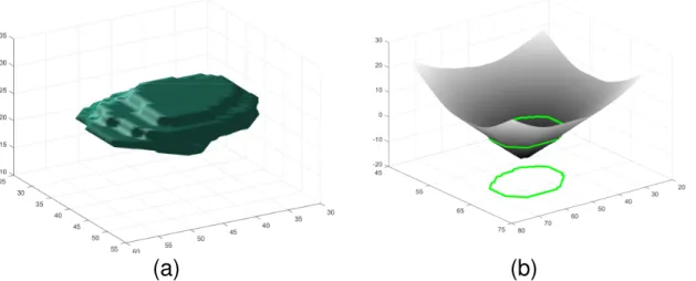
Figure 5. Representing a nodule shape by a Signed Distance Function (SDF). Left: zero level set of the SDF, Right: the SDF of a mid slice of the nodule shape, superimposed with nodule boundary shown in green on the surface and also projected onto the x-y plane. For any point, SDF encodes the closest distance to the boundary. For points inside the boundary SDF<0 and for points outside of the boundary SDF

>0.

if x is inside the surface. Locations where φ crosses zero represent the bounding surface. Fig. 5 shows construction of the SDF for an arbitrary nodule shape. Fig. 5(a) shows the nodule and Fig. 5(b) displays the SDF of mid slice of this nodule.

With embedding the surface C inside the zero level set of the SDF φ, equation (1) may be written as:

Ecv(φ) =k1 Z Ω | ∇H(φ(x))|dx +k2 Z Ω H(φ(x))dx +k₃ Z Ω (I−µ)2H(φ(x))dx +k4 Z Ω (I−ν)2(1−H(φ(x)))dx, (2)

(32)

where∇ is the gradient operator and H is the Heaviside function defined as: H(z) =        1, if z ≥0 0, if z <0 .

To minimizeEcv, the Euler-Lagrange equation is derived andφis iteratively updated:

∂φ ∂t =δ(φ)[k1div( ∇φ | ∇φ |)−k2−k3(I−µ) 2₊_k 4(I−ν)2]. (3)

In (3), the symbol div refers to the divergence operator and div(∇φ

|∇φ|) computes

the curvature of the isosurfaces embedded inφ. Further details about these and the numerical implementations can be found in [10]. To simplify subsequent descriptions, (3) is rewritten as:

φ(t+ 1) =φ(t) +Vcv(t), (4)

whereVcv(t) is the product of the right hand side of equation (3) and the time step, and is the amount of update for each iteration.

2 Shape Prior Modeling

One challenge in shape based segmentation is the alignment problem; to measure shape variations it is essential to compare like parts of shapes. Leventon, et al. [50] showed that SDFs are robust to slight misalignment helping avoid exact registra-tion. Thus, in the proposed algorithm, prior to performing segmentation, shapes are roughly aligned by computing the center of SDFs; subsequently applying an intrinsic alignment method as proposed by Cremer,et al. [21]. The center of any input shape

(33)

φ is computed from: µφ= Z Ω xh(φ(x))dx, h(φ(x)) = R H(φ(x)) ΩH(φ(x)) dx . (5)

The new shapeφ is then translated so that its center is aligned with the center of a selected reference shapeφ0.

To start building the shape prior, all registered SDFs (ϕi;i= 1, ..., n) are vector-ized and stored in columns (bases) of a matrix D = [ϕ1|ϕ2|...|ϕn] ∈ Rm×n referred to as the dictionary with each column called an atom. Here, m is the number of voxels in each training image and n is the size of the training shapes. New shapes are modeled by a linear subspace of dictionaryD. Specifically, having the dictionary

D, any new SDFφ ∈Rm may be approximated as

φ 'φ˜(x) =Dx, (6)

where x ∈ Rn is a weight vector which determines the contribution of each train-ing shape in modeltrain-ing the new shape φ. Linear combinations of SDFs in (6) do not necessarily result in a valid SDF representation [50]. However, since the linear combination will have positive and negative values, it encodes a shape at its zero level set. Starting from the zero level set, the encoded shape is then re-initialized to generate an SDF. The vector x in (6) is chosen to minimize the error between the input shape φ and its approximation; i.e.,

argmin x 1 2kφ−Dxk 2 2. (7)

Including all the atoms in the linear approximation in (7) will result in depar-ture from the valid shape space. Thus, we seek to represent the nodule boundary

(34)

compactly by an appropriate combination of training shapes, neglecting shapes from irrelevant nodule types. To achieve this, a constraint is included to limit the number of atoms that contribute to the linear approximation. More formally, a constraint is added to (7) to minimize: argmin x 1 2kφ−Dxk 2 2 subject to kxk0 ≤k. (8)

Here, kxk₀ denotes the l₀ norm, which counts the number of non-zero elements in vector x, and the parameter k controls the sparsity of x. This problem is NP-hard in nature and cannot be solved efficiently. However, recent papers have shown that if the solution is sparse enough, thel0 constraint can be replaced by the l1 norm [28].

Adding the constraint to the objective function with a penalty termλ, equation (8) is rewritten as argmin x 1 2kφ−Dxk 2 2+λkxk1;λ≥0. (9)

Unlike (8), the optimization problem in (9) is convex and can be solved efficiently.

3 Shape prior weighting

Another interpretation for (8) is that φ is a noisy or irregular shape which needs to be reconstructed from the bases in a shape dictionary. A sparse coding based on the dictionary gives us a low dimensional representation ofφ, removing irregularities from it. However, if the irregularities are dense, or the input shape is far from the atoms in the dictionary, for a fixed non-zero value of λ in (9), φ cannot be sparsely represented. In other words, the sparse weight vectorxemerging from the dictionary

(35)

Figure 6. Top left: the zero level set of an SDF corresponding to an actual nodule boundary. Top right: the zero level set of an SDF with a structure significantly different from nodule boundaries. Bottom left: the mid plane of SDF corresponding to the actual nodule boundary with the best Dx superimposed. Bottom right: the mid plane of the arbitrary SDF together with the bestDxsuperimposed (see text).

is sufficient to construct the shape prior as well as to decide the level of contribution of shape prior in segmentation.

To better illustrate this, we investigate two cases: the first one has a boundary with an SDF that is already provided in the dictionary (top left shape in Fig. 6).

(36)

The second case is when the new shape is significantly different from all atoms in the dictionary (top right shape in Fig. 6). For the first case, by solving (9), the reconstructed shape is highly sparse, resulting from just one non-zero value in vector

x, an actual shape in the dictionary. The middle slice of the reconstructed shape is shown in the bottom left of Fig. 6 with the contour accurately delineating the input shape. On the other hand, when the input shape is not similar to dictionary atoms as in the top right of Fig. 6, a significant number of shapes in the dictionary need to participate in the linear approximation in order to form a structure similar to the input shape. The reconstructed shape, shown in bottom right of Fig. 6, is not sparse in this case – this reconstruction required more than 80% of the dictionary atoms in the linear approximation for the same value ofλin (9). Despite the large number of atoms used, the input shape cannot be accurately captured by the dictionary.

To take advantage of sparsity, the shape prior weighting is made related to the level of sparsity of vector x in (9); when the surface is evolving and is not close to a shape in the dictionary, it is primarily driven by the low level Chan-Vese energy function. Once the surface starts to form a nodule boundary, the sparsity increases and correspondingly, relative to Chan-Vese energy, the weighting for the shape prior is automatically increased. This prevents the evolving surface from leaking inside neighboring organs which have a similar range of HU.

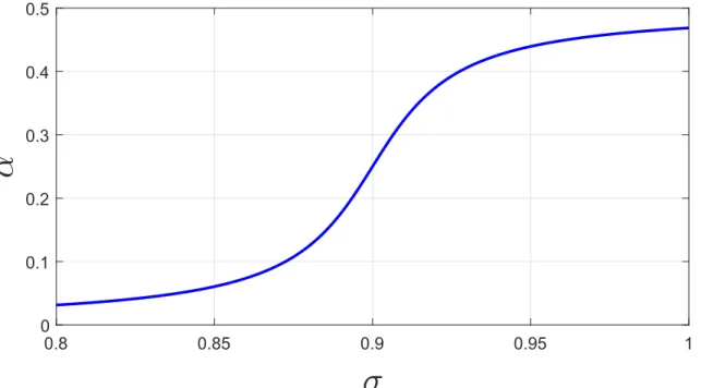
In order to map the sparsity to shape prior influence, a metric is defined so that the more sparse the representation the closer its value is to 1: σ(t) = e−s(t), where

s(t) is the sparsity ratio ofxat iteration indext, i.e, the number of non-zero elements in vector x divided by the length of the vector. The shape prior weighting plotted

(37)

0.8 0.85 0.9 0.95 1

σ

0 0.1 0.2 0.3 0.4 0.5

α

Figure 7. Shape prior weighting, α, plotted against σ (see equation (10))

in Fig. 7 is as follows,

α(σ) = tan

−1₍₅₀₍_σ₍_t₎₋₀_._{9)) +}_π/₂

2π . (10)

The saddle point of tan−1 is set to σ = 0.9 around which the shape prior weighting changes significantly.

4 Segmentation algorithm

This section provides a framework to guide the segmenting surface to separate two homogeneous regions while forcing the segmentation to be consistent with the train-ing shapes. For this purpose, we add another term to the surface evolution in (3). The new term alongside with original active contour equation helps guide the

(38)

sur-face not only by low level intensity statistics, but also by high level shape prior information. Specifically, in each step of surface evolution, it moves in a direction to optimize the Chan-Vese energy function and concurrently projects the segmenting surface into a linear subspace of training shapes. The l1 constraint in (9) provides

us the appropriate subspace.

The first term of (9) is both convex and differentiable. The second term is convex, but not differentiable. Thus, unfortunately its gradient is not well defined. For an optimization problem with this structure, a class of algorithms called coordinate-wise optimization converges to the global optimum [90]. Here, we adapt an algorithm of this class, called shooting algorithm [34], to work in conjunction with implicit surface evolution in our segmentation framework. At an abstract level, the algorithm works by fixing all the entries of solution vectorx except one, and optimizes the objective function along that dimension. That is, in each step, the algorithm moves along a specific dimension and finds the optimum value for that specific entry.

To illustrate the algorithm in more details, we introduce the following notations:

D= [ϕ1|ϕ2|...|ϕn], x= [x1, x2, ...xn],

D(−i) = [ϕ1|...|ϕi−1|ϕi+1|...|ϕn],

x(−i) = [x₁, ..., x_i₋₁, x_i₊₁, ...x_n].

The non-differentiable part of (9) can be separated into individual coordinate wise components, each of which can be solved directly by applying Karush-Kuhn-Tucker necessary conditions. By fixing the values ofx(−i), theithcoordinate wise component of (9) is obtained by solving the following:

argmin1

2kφi−ϕixik

2

(39)

whereφi =φ−D(−i)(x)(−i) is the error of the approximation computed when includ-ing all the atoms of the dictionary exceptϕi. To find the best value for the coefficient

xi, (11) minimizes the error of approximation by adding the contribution of ϕi to the linear approximation. Following the Karush-Kuhn-Tucker necessary conditions, the optimal solution is obtained as follows:

x∗_i =                (φT iϕi−λ) ϕT iϕi , if φT_i ϕ_i−λ >0. (φT iϕi+λ) ϕT iϕi , if φT_i ϕi+λ <0. 0, if −λ≤φT_i ϕi ≤λ. (12)

Equation (12) simply computes the projection of error (φi) onto theith atom of the dictionary. If the size of this projection is in [−λ, λ], xi is set to zero, otherwise its value is set to(φTiϕi−λ) ϕT iϕi or (φT iϕi+λ) ϕT

iϕi depending on whether the projection is greater than λ or less than −λ. In summary, this algorithm iteratively optimizes the objective function along one coordinate, while keeping other coordinates fixed.

Having the final approximated surface, we now can not only evolve the surface in the direction of Chan-Vese update, but also in a direction that minimizes the distance between the surface and its approximation. This update is illustrated in more details in Figure 8, where a linear combination of the Chan-Vese and shape update is computed and the surface is moved in that direction. To better illustrate equation update shown in Figure 8, we inspect two extreme cases:

α=0: in this case, the term corresponding to shape update vanishes and the surface is driven by the Chan-Vese equation. The algorithm in this case is the same as classial Chan-Vese algorithm.

(40)

Figure 8. T

he surface evolution update is computed by a linear combination of updates in the direction of the Chan-Vese and the shape approximation.

(41)

does not play any role in this case. Thus, the curve is guiding by the shape energy update and in each iteration the surface is updated rendering the approximated shape prior.

The proposed algorithm for image segmentation is illustrated in Algorithm 1. It incorporates the shooting algorithm into level set evolution and forces the surface to separate homogeneous regions and at the same time keeps it similar to a linear combination of training shapes in the dictionary.

Algorithm 1 Image Segmentation by SCoTS

1: Initializex randomly andφby the SDF of a 5×5 square 2: while kE(t+ 1)−E(t)k> T hreshold do 3: Compute approximation: ˜φ=Dx 4: update φ(t+ 1) =φ(t) +α(σ) ˜ φ(t)−φ(t) + (1−α(σ))V_cv(t) 5: for i= 1 :n do

6: using current value of x(−i) solve (11).

7: Suppose x∗_i is the solution of (11), update ith

element of x tox∗_i.

8: end for

9: Compute number of non-zeros inx and update α(σ)

10: end while

In this algorithm, ˜φ represents sparse approximation of the evolving surface. The shape prior weighting function α(σ) determines the level of trust in the shape prior and is a function of sparsity (10). The algorithm consists of two nested loops. In the outer loop the segmenting surface gets updated in the direction of a linear combination of Chan-Vese and sparse shape prior terms. The inner loop refines the updated shape and brings it into the valid shape space.

(42)

5 Convergence and Complexity

Convergence

The stopping criterion for the proposed algorithm is based on the change in the energy of the segmenting surface. If the energy does not change from one iteration to the next, the algorithm stops. We define the energy function as the sum of the Chan-Vese energy function and the computed sparse linear approximation.

E(φ(t),x(t)) = Ecv(φ(t)) +Esp(φ(t),x(t)). (13)

E_cv is the Chan-Vese energy function and E_sp is the energy term defined in (9). Although convergence of the algorithm cannot be mathematically proven, we have empirically observed that as long as the evolving surface is roughly initialized at the center of the nodule, the algorithm converges.

Time Complexity

The algorithm complexity is a function of Chan-Vese and shape approximation com-plexity. In each iteration of the outer loop, one iteration of Chan-Vese, as well as n iterations of the inner loop are applied. The inner loop solves (11) through conditions provided in (12). However, as pointed out in [72], all the required values ofφT_i ϕi and

ϕT_i ϕi for (12) can be pre-computed before starting the inner loop. Thus, since the complexity of Chan-Vese in each iteration isO(N ×M ×P), where N ×M ×P is the size of the image, the complexity of one iteration of the proposed algorithm is

(43)

CHAPTER IV

SEGMENTATION RESULTS

1 Dataset

The proposed algorithm for nodule segmentation has been validated on a subset of data form the lung image database consortium image collection (LIDC-IDRI) [4, 18]. In LIDC-IDRI, each dataset is a breath-held 3D CT image of the thorax with size 512×512. The number of slices varying between 95 and 672 and the in-plane pixel size varies between 0.5 and 0.8 mm/pixel. The range for the kVp for these data was 120-140 with 120 as the average and 20.99 as the standard deviation. The range for the mA was 30-634 with 215.9 as the average and 145.1 as the standard deviation. LIDC-IDRI contains lung CT scans from 1018 patients with nodule annotations provided by four experienced radiologists. It should be noted that the 4 radiologists who delineated the LIDC data differ between cases so that not the same 4 individuals read and delineated each scan. Therefore, for the rest of the paper, the reader should keep in mind that ”radiologist j’s delineations” (j=1, ..., 4) can indeed be from a number of individual radiologists.

Since nodules of size less than 3 mm are considered inconsequential, for our validation we only included data with nodule size greater than or equal to 3 mm in

(44)

diameter. Furthermore, we selected those nodules that were in common among all four radiologists. This left 542 nodules that fit inside predefined cubic volumes.

2 Evaluation

The approach adopted to validation is 10 fold cross validation [45], four times, once for each radiologist’s delineations. That is, 542 nodules as delineated by each radiol-ogist were divided into 10 groups (folds). The SDFs of shapes corresponding to the nodules of 9 folds served as the atoms of the dictionary and the algorithm was tested on nodules in the 10th fold. The testing fold was successively changed between the 10 groups, each providing a different segmentation accuracy.

The accuracy of segmentation is measured based on the Dice Similarity Coefficient (DSC), Jaccard index (J), True Positive Rate (TPR), and False Positive Rate (FPR):

DSC = 2N(A∩B) N(A) +N(B), T P R= T P T P +F N, J = N(A∩B) N(A∪B) = DSC 2−DSC, F P R= F P F P +T N, (14)

where in (14),A denotes the set of voxels classified by the algorithm to belong to the lung nodule, B is the ground truth from manual delineation,N(V) is the voxel count in the setV,T P is the number of nodule voxels correctly segmented by the algorithm,

F N represents the number of nodule voxels mistakenly segmented as background,

F P is the number of non-nodule voxels mistakenly segmented as belonging to the nodule, and T N is the number of non-nodule voxels that are correctly segmented.

For more detailed evaluations, we also classified the nodules into several categories based on texture and attachment. Information about nodules texture may be found

(45)

in the LIDC XML Base Schema [1], where each radiologist rated the lesions related to in several categories including texture. The texture was classified from (1-5), where label 5 indicates solid nodules, label 3 corresponds to part-solid, and label 1 represents non-solid nodules. From the selected dataset, we chose nodules for which more than one radiologist’s rating was part-solid or non-solid. The selected subset contained 37 samples which met this criterion. In addition to this classification, a thoracic radiologist (Dr. Seow) further classified the nodules in our LIDC-IDRI datasets. It turned out 209 nodules are well-circumscribed, 178 are juxta-vascular while the total number of juxta-pleural and pleural tail nodules combined is 155. Since only a small fraction of nodules were classified as pleural tail, we combined these with juxta-pleural nodules.

3 Parameters Settings

The algorithm works on a region of interest (ROI) with size 75×85×45 with the nodule approximately centered. The approach to selection of the ROI was to keep the ROI size (in voxels) large enough to include all the nodules in the dataset. We extracted the size of all nodules as delineated by radiologists and determined the number of voxels they occupy in each dimension for the dataset. The largest number of voxels occupied for all nodules was 71 in the first dimension, 80 in the second dimension and 35 in the third dimension. We picked 75×85×45 for the size of ROI to ensure that all nodules delineated by all radiologists would fit inside the ROI.

The algorithm’s parameters were determined through optimization of the Dice Similarity Coefficient (DSC) for a limited number of samples of the three nodule

(46)

Table 1. The algorithm parameters values used for all experiments

Parameter

k

1

k

2

k

3

k

4

λ

Value

0 .

2

0

5

150

classes: well-circumscribed, juxta-pleural, and juxta-vascular. Following this ap-proach we arrived at parameter values in Table 1.

In applying the segmentation algorithm, a point at the center of nodule is selected manually around which a 5×5 square was prescribed as the zero level set of an SDF which iteratively evolved into a 3D shape and into neighboring slices.

4 Results

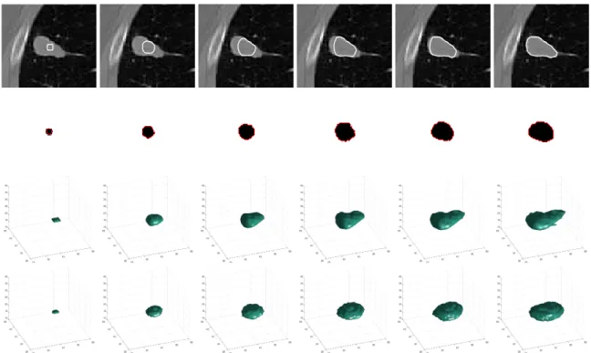
The first experiment, illustrated in Fig. 9, demonstrates the surface and shape evolution through different steps. The initial and final segmenting surface are shown in the first and last columns of this figure respectively. Also, a few intermediate steps of segmentation are shown in the second to fifth columns of this figure. The zero level set of adaptive shape prior and its evolution has also been shown in the second and fourth rows. As the segmenting surface evolves, the shape prior changes and adapts itself to the segmenting surface. For this experiment, each iteration of the algorithm approximately took 7.3 seconds of CPU time in MATLAB on an AMD 3.9 GHz with 32 GB RAM of memory. The algorithm converged after 50 iterations and segmented the volume in 6 minutes.

A second result is used to demonstrate the evolution and convergence of the sparse representation. Fig. 10(a) shows the mid slice of an input nodule superimposed with

(47)

Figure 9. Surface and adaptive shape prior evolution. First column corresponds to the initialization. Columns 2-6 show iterations 6, 13, 20, 27, and the final result in iteration 50. First and third row show the evolution of segmentation in 2D and 3D respectively and second and fourth rows show the zero level set of adaptive shape prior in 2D and 3D.

the segmentation surface plotted in red. Fig. 10(b) shows this nodule in three dimensions delineated by the radiologist. Fig. 10(c) shows the final segmenting surface. Shape prior constructed from dictionary atoms is shown in Fig. 10(d). Fig. 10(e) and Fig. 10(f) represent two shapes from the dictionary that had significant contribution in building the shape prior. Fig. 10(g) shows the evolution of vector x

(equation (6)) over 100 iterations of the algorithm. Every iterative update of vector

x is stored as a column of a matrix with increasing iterations going from left to right. Small entries are shown in blue and for some the color shifts towards red as

(48)

the iterations and values increase. For the sake of simplicity only those entries of vector x that changed were shown in this figure. We can see that for the first 20 iterations, selected atoms varying from one iteration to another. Subsequently, the algorithm promotes few atoms, two of which were shown in Fig. 10(e) and 10(f). This result is quite typical for the algorithm in that any valid nodule shape can be represented by 1−3% of the shape atoms in the dictionary. In Fig. 10(h) the total energy (equation (13)) is plotted over 100 iterations. The plot shows that the total energy converges and does not change significantly after 30 iterations. Finally, in Fig. 10(i), shape energy is presented. Initially, the shape energy oscillates with no apparent intention to converge. However, once the evolving surface forms a nodule boundary structure, the shape energy starts to decrease, resulting in convergence.

Fig. 11 shows segmentation of some samples of LIDC-IDRI dataset. It demon-strates how the proposed algorithm can distinguish the nodule from the surrounding tissues like vessel or pleura. It can be seen that when the nodule is not spherical, the proposed method can still capture the nodule. The last row in this figure shows samples for which the algorithm did not generate satisfactory results. The reason behind the failures maybe attributed to the fact that the framework is general and tries to segment all types of nodules. Failures mostly happen in situations where the nodules are attached to organs with similar HUs and at the same time the shape prior of the nodule cannot be sparsely reconstructed from the dictionary. As a result, the shape prior energy is dominated by Chan-Vese energy function and the segment-ing surface leaks into adjacent regions. Another type of failure is related to very small and non-solid textured nodules which pose difficulty for Chan-Vese algorithm

(49)

(a)

50 48 46 44 42 40 38 15 44 42 40 38 ₃₆ 36 34 32 30 20 25 30

(b)

48 46 44 42 40 15 44 43 42 41 40 ₃₉ 38 38 37 36 35 34 20 25 30

(c)

48 46 44 42 40 18 44 43 42 41 40 ₃₉ 38 38 37 36 35 34 20 22 24 26 28

(d)

50 48 46 44 42 40 38 15 46 44 42 ₄₀ 36 38 36 34 20 25 30

(e)

48 46 44 42 40 18 44 42 40 ₃₈ 38 36 34 32 20 22 24 26 28

(f)

20 40 60 80 100 Iteration 20 40 60 Weight vector (x) 0 0.05 0.1 0.15 0.2 0.25 f e

(g)

0 10 20 30 40 50 60 70 80 90 100 Iteration 1.5 2 2.5 3 3.5 4 4.5 Shape Energy ×106

(h)

0 10 20 30 40 50 60 70 80 90 100 Iteration 0.9 1 1.1 1.2 1.3 1.4 1.5 1.6 1.7 1.8 1.9 Shape Energy ×106

(i)

Figure 10. (a) Mid slice of a nodule and its boundary, (b) ground truth nodule boundary in 3D, (c) segmented boundary in 3D, (d) shape prior constructed from dictionary atoms, (e,f) dictionary atoms with highest weights in nodule boundary reconstruction, (g) evolution of column vector x(only 75 elements of the vector are shown) over 100 iterations - the weight of atoms corresponding to shapes (e) and (f) are distinct in yellow and red colors with arrows pointing to them. The range of weights during evolution for elements of the vector x was [0,0.23]. (h,i) total energy and shape energy over 100 iterations of the algorithm.

(50)

Table 2. Numerical validation of the algorithm (DSC, TPR, FPR) on 542 nodule CT dataset using Radiologist j’s delineations for both training and testing with 10 fold cross validation. When rounded to the nearest hundredth, for all cases FPR was zero and therefore has not been included in the table. In this approach all delineations from each radiologist is randomly split into 10 groups (folds). Delineations in 9 of the folds are used to construct the dictionary. The image data in the 10th fold are used for testing. See text for additional descriptions.

Radiologist 1 Radiologist 2 Radiologist 3 Radiologist 4 SCoTS DSC= 0.72±0.15 DSC= 0.71±0.17 DSC= 0.72±0.16 DSC= 0.71±0.17

T P R= 0.77±0.16 T P R= 0.8±0.16 T P R= 0.77±0.17 T P R= 0.78±0.16

to grow properly. For such cases, the shape prior energy is dominant (see last row of Fig. 11). These nodules have shapes that does not appear in the training set. Such a nodule when attached to a vessel or pleura poses a challenge to the algorithm. In this case, neither the density nor proposed shape prior information stops the surface from growing into surrounding tissues.

In Table 2 we report the segmentation accuracy of SCoTS with respect to each radiologist’s delineations separately. Column j reports the accuracy when radiologist j’s delineations were used to build the dictionary. Subsequently, 10 fold cross valida-tion was performed based on this dicvalida-tionary. The average DSC and TPR for each of the 10 testing folds were averaged in order to produce the entries in the table.

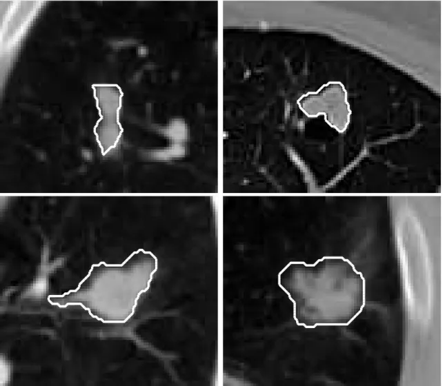
Although in Table 2 the segmentation accuracies are very close to one another, the segmented nodules are not identical and in some cases even dissimilar. Fig. 12 shows four images in which dictionaries constructed from different experts’ delin-eations produced significantly different segmented surfaces. In this figure, red, blue, green, and yellow curves identify the final segmentation produced by a dictionary constructed from nodules delineated by radiologist number 1, 2, 3, and 4

(51)

respec-Figure 11. Segmentation of some samples of the lung dataset. Segmented bound-aries were painted in white color. For these results, the dictionary was built based on radiologists 1’s delineations followed by the 10 fold cross validation approach. Top 7 rows represent cases where the algorithm successfully segmented out the nodule from surrounding tissues. The last row shows 7 cases where the algorithm did not generate satisfactory results. These nodules have shapes that may not appear in the training set. We define failure cases as samples which have DCS less than 0.6. By this definition, the average percentage of failure over all samples is 13.5%.

(52)

Figure 12. Segmentation results based on dictionaries built based on first, second, third, and fourth radiologists’ delineations. For each case, different colors repre-sent different dictionaries. The figure illustrates the resulting variability of the final segmentation.

tively. This behavior suggests the possibility of combining the results in a consensus manner where the segmented surfaces obtained by each dictionary are fused by an aggregation method such as [94] to provide higher accuracies.

To assess inter-observer variability in LIDC-IDRI database, radiologists’ delin-eations are compared to each other in Table 3. In this table and for column j, radiologist j’s delineations were used as the ground truth for direct comparison with the radiologist in row i. The table confirms inter-observer variability as the computed DSC and TPR are not exactly equal to 1. Therefore, we provide another validation in Table 4 based on a consensus scheme with four radiologists’ delineations known as simultaneous truth and performance level estimation (STAPLE) [94]. In a cap-sule, STAPLE works by jointly optimizing the TPR and the FPR in an expectation maximization framework. It generates a probabilistic estimate for each voxel which when thresholded over 0.5 produces a consensus mask as ground truth. In Table 4 this mask has been used as ground truth. More specifically, in producing the en-tries in column j of this table, 9 folds of radiologist j’s delineations were used as

(53)

Table 3. Inter-observer variability among four radiologists for delineation of nodules in the LIDC-IDRI database. Reported in rows i column j is the DSC and TPR for radiologists i using radiologist j delineations as ground truth. When rounded to the nearest hundredth, for all cases, FPR was zero and therefore has not been included in the table.

Radiologist 1 Radiologist 2 Radiologist 3 Radiologist 4 Radiologist 1 DSC= 1 DSC= 0.79±0.09 DSC= 0.80±0.10 DSC= 0.79±0.10 T P R= 1 T P R= 0.85±0.13 T P R= 0.84±0.13 T P R= 0.82±0.13 Radiologist 2 DSC_{T P R}_{= 0}= 0._.₇₈79±0.09 DSC= 1 DSC= 0.81±0.10 DSC= 0.79±0.10 ±0.14 T P R= 1 T P R= 0.81±0.15 T P R= 0.79±0.14 Radiologist 3 DSC= 0.80±0.10 DSC= 0.81±0.10 DSC= 1 DSC= 0.79±0.10 T P R= 0.79±0.14 T P R= 0.84±0.14 T P R= 1 T P R= 0.80±0.14 Radiologist 4 DSC_{T P R}_{= 0}= 0._.₇₉79±0.10 DSC= 0.79±0.10 DSC= 0.79±0.10 DSC= 1 ±0.16 T P R= 0.83±0.15 T P R= 0.82±0.14 T P R= 1

Table 4. Numerical validation of the algorithm (DSC, TPR, FPR) on 542 nodule CT dataset using Radiologist j’s delineations for training and STAPLE for testing with 10 fold cross validation. When rounded to the nearest hundredth, for all cases, FPR was zero and therefore has not been included in the table.

Radiologist 1 Radiologist 2 Radiologist 3 Radiologist 4 SCoTS DSC= 0.73±0.16 DSC= 0.74±0.16 DSC= 0.73±0.16 DSC= 0.73±0.16

T P R= 0.84±0.14 T P R= 0.77±0.15 T P R= 0.75±0.17 T P R= 0.77±0.15

dictionary and the output of SCoTS on test nodules in the 10th fold were compared with the ground truth from STAPLE. Comparing tables 2 and 4, the ground truth obtained by STAPLE resulted in higher accuracy compared than the case where one radiologist’s delineation served as the ground truth (Table 2).

To evaluate how SCoTS performs on different nodule classes, the relevant DSC and TPR values were evaluated on different nodule classes – results are reported in Table 5. Similar to Table 2, dictionary construction and ground truth alternates between four radiologists in a round robin fashion. It can be seen that performance is best on well-circumscribed nodules, and lowest on juxta-pleural/pleural tail nodules.

(54)

Table 5. Performance of SCoTS on specific nodule types.

Radiologist 1 Radiologist 2 Radiologist 3 Radiologist 4 Well-circumscribed DSC= 0.75±0.14 DSC= 0.75±0.13 DSC= 0.75±0.13 DSC= 0.75±0.13

T P R= 0.78±0.17 T P R= 0.79±0.15 T P R= 0.77±0.17 T P R= 0.79±0.16 Juxta-vascular DSC= 0.73±0.14 DSC= 0.73±0.13 DSC= 0.72±0.16 DSC= 0.73±0.14

T P R= 0.74±0.16 T P R= 0.73±0.16 T P R= 0.70±0.19 T P R= 0.73±0.16 Juxta-pleural & plural tail DSC_{T P R}= 0_{= 0}._.₇₈64±0.20 DSC= 0.62±0.23 DSC= 0.64±0.20 DSC= 0.63±0.22

±0.17 T P R= 0.78±0.18 T P R= 0.77±0.17 T P R= 0.78±0.17

This is not surprising because these are the least and most challenging cases respec-tively. Another observation is that no matter which radiologist’s delineations were used to construct the dictionary, SCoT’s performance is similar on well-circumscribed nodules. We see reduction in performance on juxta-pleural and pleural tail nodules.

Table 6 compares results of SCoTS to other nodule segmentation methods which have been tested on the LIDC-IDRI database. Although all papers cited in Table 6 make use of the LIDC-IDRI database for validation, their experimental setup are different from our approach. The approach to validation in [11] split samples from the LIDC database into two groups, training the model on one group and testing on the second group without any cross validation. The authors of [49] used around 100 nodule data to build their model, and although they used the LIDC-IDRI data for testing, they did not specify if the training data were from the LIDC-IDRI database or from another database. While the method proposed in [8] used the LIDC-IDRI database for testing, it did not involve any training. The method in [5] also did not involve any training but for testing, the authors of [5] used the same nodule data sets in the LIDC-IDRI database that we have used for our training and testing. To compare our results with [5], a voxel probability map metric used in [5] was

(55)

Table 6. Comparison of performance of SCoTS with previously proposed nodule segmentation methods applied to LIDC-IDRI data. For this table, the dictionary used was built by radiologist 1’s delineations, followed by 10 fold cross validation. First three rows compares SCoTS with two other methods considering all nodule types. The next two rows compares SCoTS with [11] on juxta-vascular nodules and the last two rows compares SCoTS with [49] considering only non-solid or part-solid nodules. We report TPR withMpr = 100% as done for MRFC-OB [5] for SCoTS.

T P R

(%)

F P R

(%)

J

SCoTS

90 .

26 _±

11 .

42

0 .

3 _±

0 .

5

0 .

57 _±

0 .

16 MRFC-OB [16]

95 .

50 _±

7 .

86 N/A

N/A

Cavalcanti,

et al.

[17]

93 .

53

0 .

89 N/A

SCoTS (JV)

88 .

91 _±

11 .

74

0 .

13 _±

0 .

46

0 .

57 _±

0 .

14 Chen,

et al.

[12]

88 .

89

10 .

19 N/A

SCoTS (non/part-solid)

81 .

73 _±

23 .

57

0 .

9 _±

1 .

2

0 .

36 _±

0 .

23 Lassen,

et al.

[14]

N/A

0 .

50 _±

0 .

14

calculated for SCoTS. The map is computed for each voxelcof the nodule as follows: if all radiologists classifycas being part of the nodule, then the Mpr(c) = 100%. At the other extreme, if c is not assigned a nodule label by any of the radiologists, then MP R(c) = 0%. Based on this definition, T P R is defined as true positive rate computed with Mpr(c) = 100% as ground truth. Further details about this metric can be found in [5]. Table 6 compares the segmentation accuracies based on T P R

and Jaccard index (J) defined in (14).

Despite the fact that results in [5] are better than SCoTS, we should point out that in [5] each nodule class is treated separately with a different segmentation ap-proach. In [5] after applying Otsu thresholding, a connectivity analysis was done to determine the nodule type, separating juxta-vascular and well-circumscribed nodules from juxta-pleural and pleural tail nodules. Attached tissues were separated from

(56)

pleural tail or pleural surface either by morphological operations or a thickening al-gorithm. However, SCoTS extracts the nodule shape by sparse representation and without any preprocessing or classification step in advance. Also, the method pro-posed in [8] needs an ROI as the input to the algorithm, used as a reference slice for background without nodule tissue. From this point of view, the proposed method is more general since it does not require the user to provide nearest slice to lesion.

The performance of the SCoTS on juxta-vascular nodules (SCoTS (JV)) is also shown in Table 6. Despite the close accuracy, the method in [11] is applicable to juxta-vascular nodules and in this sense less general than the method proposed in this paper.

From the last two rows of Table 6, it can be seen that SCoTS does not perform well on non-solid and part-solid nodules. The main reason for this diminished per-formance lies in the Chan-Vese energy function and not shape prior energy. The Chan-Vese algorithm tries to separate homogeneous regions from ROI whereas the non-solid nodules have inhomogeneous appearance and pose difficulty for SCoTS. However, it should be noted that the algorithm in [49] requires additional manual steps as the user is required to draw the largest diameter of the nodule.

(57)

CHAPTER V

DEEP LEARNING IN MEDICAL IMAGE ANALYSIS

Traditionally Computer Aided Diagnosis (CAD) systems have relied on handcrafted features and classifier systems to distinguish between benign and malignant patholo-gies. With the advent of deep learning systems, optimum features are learned for the classification task at hand. This chapter reviews fundamentals of deep learning and its success in medical image detection, segmentation, and diagnosis of anatomical objects.

Type equation here.

𝑖