Matlab/Octave toolbox for structurable and robust output-feedback
LQR design
Downloaded from: https://research.chalmers.se, 2019-05-11 11:40 UTC
Citation for the original published paper (version of record):
Ilka, A. (2018)
Matlab/Octave toolbox for structurable and robust output-feedback LQR design
Preprints of the 3rd IFAC Conference on Advances in Proportional- Integral-Derivative Control, 51(4):
N.B. When citing this work, cite the original published paper.
research.chalmers.se offers the possibility of retrieving research publications produced at Chalmers University of Technology. It covers all kind of research output: articles, dissertations, conference papers, reports etc. since 2004.
research.chalmers.se is administrated and maintained by Chalmers Library
Matlab/Octave toolbox for structurable
and robust output-feedback LQR design
?
Adrian Ilka
Department of Electrical Engineering,
Chalmers University of Technology, H¨orsalsv¨agen 9-11, SE-412 96, Gothenburg, Sweden. E-mail: [email protected]
www.adrianilka.eu
Abstract: In this paper, a structurable robust output-feedback infinite horizon LQR design toolbox for Matlab and Octave is introduced. The aim of the presented toolbox is to fill the gap between available toolboxes for Matlab/Octave by extending the standard infinite horizon LQR design (from Matlab/Control System Toolbox, Octave/Control package) to robust and structurable output-feedback LQR design. The toolbox allows to design a robust infinite horizon output-feedback controller in forms like proportional (P), proportional-integral (PI), realizable proportional-integral-derivative (PID), realizable proportional-derivative (PD), realizable derivative (D), dynamic output-feedback (DOF), dynamic output-feedback with integral part (DOFI), dynamic output-feedback with integral and realizable derivative part (DOFID), and dynamic output-feedback with realizable derivative part (DOFD). In addition, the controller structure for all supported controller types is fully structurable. The toolbox relies on Yalmip (A Matlab/Octave Toolbox for Modeling and Optimization) and on linear matrix inequality solvers like SeDuMi, SDPT3, etc. Notions like ”simple”, ”highly customizable”, and ”user-friendly” have been used and considered as main terms during the development process.
Keywords:Linear quadratic regulator, Robust control, Output-feedback, Structured controller.
1. INTRODUCTION
One of the most fundamental problems in control theory is the linear quadratic regulator (LQR) design problem (Kwakernaak and Sivan, 1972). The so-called infinite hori-zon linear quadratic problem of finding a control function
u∗∈Rmforx
0∈Rn that minimizes the cost functional:
J∗= Z ∞ 0 x(t)TQx(t) +uT(t)Ru(t) + 2xT(t)N u(t)dt, (1) with R > 0, Q− N R−1NT ≥ 0 subject to ˙x(t) =
Ax(t) + Bu(t), x(0) = x0 has been studied by many
authors (Kwakernaak and Sivan, 1972; Willems, 1971; Molinari, 1977; Trentelman and Willems, 1991). However, many times, it is not possible or economically feasible to measure all the state variables. Therefore, several new algorithms have been developed that resulted in gener-alization of the above state-feedback problem to output-feedback (Vesel´y, 2001; Rosinov´a et al., 2003; Engwerda and Weeren, 2008; Mukhopadhyay, 1978). Subsequently, the robust static output-feedback version of the LQR design has also been studied in many papers (Rosinov´a and Vesel´y, 2004; Vesel´y, 2005, 2006), as well as the LQR-based proportional-integral-derivative (PID) controller de-sign (Rosinov´a and Vesel´y, 2007; Vesel´y and Rosinov´a, 2011, 2013). The introduction of linear parameter-varying (LPV) systems (Shamma, 2012) has opened new
possi-? This work has been financed in part by the Swedish Energy Agency
(P43322-1), and by IMPERIUM (H2020 GV-06-2015).
bilities in LQR design. Several gain-scheduled/LPV-based LQR design techniques appeared in both static output feedback (SOF) and dynamic output-feedback (DOF), not to mention the PID controller design (Vesel´y and Ilka, 2013; Ilka and Vesel´y, 2014; Vesel´y and Ilka, 2015a; Ilka et al., 2016, 2015; Vesel´y and Ilka, 2015b, 2017; Ilka and Vesel´y, 2017a; Ilka and McKelvey, 2017; Ilka and Vesel´y, 2017b).
From this short literature survey follows that necessity for preparing a toolbox for LQR-based output-feedback approaches has come to the fore. The plan is to pre-pare and collect a bunch of functions for structurable LQR-based output-feedback controller design which can be used with Matlab and Octave as well. In this paper, one of the functions prepared for the toolbox (oflqr
function) is presented. This function allows to design a robust infinite horizon output-feedback controller in forms like proportional (P), proportional-integral (PI), realizable proportional-integral-derivative (PID), realiz-able proportional-derivative (PD), realizrealiz-able derivative (D), dynamic feedback (DOF), dynamic feedback with integral part (DOFI), dynamic output-feedback with integral and realizable derivative part (DOFID), and dynamic output-feedback with realiz-able derivative part (DOFD), for uncertain linear time-invariant (LTI) systems with polytopic uncertainty. In ad-dition, the controller structure for all supported controller types is fully structurable. The function relies on Yalmip (L¨ofberg, 2004) and on linear matrix inequality solvers like SeDuMi (Sturm, 1999), SDPT3 (Toh et al., 1999) etc.
The rest of the paper is organized into four sections. The introduction is followed by a theoretical background of the presented function in Section 2. The oflqr function is described in Section 3, and numerical examples are given in Section 4. Finally, Section 5 closes the paper with some concluding remarks.
The mathematical notation of the paper is as follows. Given a symmetric matrixP =PT ∈
Rn×n, the inequality
P > 0 (P ≥ 0) denotes the positive definiteness (semi definiteness) of the matrix. Matrices, if not explicitly stated, are assumed to have compatible dimensions. I
denotes the identity matrix of corresponding dimensions.
2. THEORETICAL BACKGROUND
Consider the following uncertain linear time-invariant (LTI) system with polytopic uncertainty as follows:
˙
x(t) =A(ξ(t))x(t) +B(ξ(t))u(t),
y(t) =C(ξ(t))x(t) +D(ξ(t))u(t). (2)
where x(t) ∈ Rn, y(t) ∈
Rl, and u(t) ∈ Rm are the
state, measurable output, and the control input vectors, respectively. Matrices A(ξ(t))∈ Rn×n, B(ξ(t))∈ Rn×m,
C(ξ(t))∈Rl×n andD(ξ(t))∈Rl×mbelong to the convex
set, a polytope withpvertices that can be formally defined as: Ξ :=nS(ξ(t)) = p X j=1 Sjξj(t), p X j=1 ξj(t) = 1, ξj(t)≥0 (3)
Remark 1. In the system (2), the matrix D(ξ(t)) can be assumed, without loss of generality, to be zero, see (Zhou et al., 1996).
The function oflqr allows to design different controller types such as P, PI, PID, PD, D, DOF, DOFI, DOFID and DOFD. The output-feedback control law for controller type DOFID can be defined as:
˙ xc(t) =−Acxc(t)−Bc1y(t)−Bc2 Z t 0 yi(t)dt −Bc3ydf(t) u(t) =−Ccxc(t)−Kpy(t)−Ki Z t 0 yi(t)dt −Kdydf(t) (4)
where, xc ∈ Rnc is the state vector of the dynamic
controller, yi ∈ Rli is the measurable output vector for
the integral part,ydf ∈R
ldis the vector of filtered output
derivatives using a derivative filter with filter coefficient
Nf: Gf(s) = Nfs s+Nf . (5) Matrices Ac ∈Rnc×nc, B c1 ∈R nc×l,B c2 ∈R nc×li, B c3 ∈ Rnc×ld, C
c ∈ Rm×nc, are the controller’s gain matrices
related to the dynamic controller, furthermoreKp∈Rm×l,
Ki∈Rm×liandK
d∈Rm×ldare the proportional, integral
and derivative gain matrices, respectively.
For the controller design, the system (2) is augmented (with the assumption thatD= 0, see Remark 1) with the state vector of the dynamic controllerxc(t), with integral
of the outputs for the integral part z(t) = R0tyi(t)dt, and
with the filtered outputs for the controller’s derivative part
yf(t): ˙˜ x(t) =Aaug(ξ(t))˜x(t) +Baug(ξ(t))˜u(t) ˜ y(t) =Caug(ξ(t))˜x(t) (6) where ˜x(t)T = [x(t)T, x c(t)T, z(t)T, yf(t)T] is the
aug-mented state vector, ˜y(t)T = [y(t)T, xc(t)T, z(t)T, ydf(t)
T]
is the augmented output vector, ˜u(t) = [u(t)T, x
c(t)T] is
the augmented control input vector, and
Aaug(ξ(t)) = c1 c2 c3 c4 r1 A(ξ(t)), 0n×nc, 0n×li, 0n×ld r2 0nc×n, 0nc×nc,0nc×li,0nc×ld r3 Ci(ξ(t)), 0li×nc, 0li×li, 0li×ld
r4 BfCd(ξ(t)),0ld×nc, 0ld×li, Af , Baug(ξ(t)) = c1 c2 r1 B(ξ(t)),0n×nc r2 0li×m, Ili×nc r3 0li×m, 0li×nc r4 0ld×m, 0ld×nc , Caug(ξ(t)) = c1 c2 c3 c4 r1 C(ξ(t)), 0l×nc, 0l×li, 0l×ld r2 0nc×n, Inc×nc,0nc×li,0nc×ld r3 0li×n, 0li×nc, Ili×li, 0li×ld
r4 BfCd(ξ(t)),0ld×nc, 0ld×li, Af
,
where Ci(ξ(t)) ∈ Rli×n is the output matrix for the
integrals, and Cd(ξ(t)) ∈ Rld×n is the output matrix for
the derivatives.
Finally, for the controller design the control law (4) is transformed to a form: u(t) =Fy˜(t) =F Caug(ξ(t))˜x(t), (7) where F = c1 c2 c3 c4 r1 Kp, Cc, Ki, Kd r2 Bc1, Ac, Bc2, Bc3 .
Remark 2. For controller types P, PI, PID, PD, D, DOF, DOFI or DOFD one can simply neglect the unwanted parts (rows/columns of dynamic, integral or derivative parts) from (6) and (7).
Remark 3. The structure of the gain matrices can be predefined. Moreover, a fully decentralized control can be achieved (if m = l), by defining the gain matrices in diagonal form.
Theorem 1. For the uncertain LTI system (2) an optimal (suboptimal) stabilizing controller exists in the form (4) minimizing the cost function (1), if for the given positive definite matrix X, and weighting matrices Q, R and N, the following problem has a solution:
min F,P trace(P), (8) subject to LMIs: Mj ≤0, j= 1, . . . , p (9) P >0 (10) where Mj= ATaugjP+P Aaugj +Q+Hj, G T j Gj, −R−1 , (11) Gj =F Caugj −R −1BT augjP+N T, (12)
Hj=−(XBaugj +N)R −1(BT augjP+N T) −(P Baugj+N)R −1(BT augjX+N T) +(XBaugj +N)R −1(BT augjX+N T). (13)
Proof 1. Let us choose the Lyapunov function as:
V(t) = ˜x(t)TPx˜(t), (14) The first derivative of the Lyapunov function (14) is then:
˙
V(ξ(t)) = ˙˜x(t)TPx˜(t) + ˜x(t)TPx˙˜(t)
= ˜x(t)T Ac(ξ(t))TP+P Ac(ξ(t))x˜(t),
(15)
where
Ac(ξ(t)) =Aaug(ξ(t)) +Baug(ξ(t))F Caug(ξ(t)). (16)
By substituting the control law (7) to the cost function (1) we can obtain: J∞= Z ∞ 0 ˜ x(t)TJ(ξ(t))˜x(t)dt (17) where J(ξ(t)) =Q+Caug(ξ(t))TFTRF Caug(ξ(t)) +N F Caug(ξ(t)) +Caug(ξ(t))TFTNT. (18)
By summarizing the equations (15) and (18) the Bellman-Lyapunov inequality can be obtained in the form:
M(ξ(t)) = ˙V(ξ(t)) +J(ξ(t))≤0, (19) Furthermore, if P is positive definite then the Bellman-Lyapunov inequality (19) can be rewritten to this form:
˙
V(ξ(t)) +J(ξ(t))≤0→V˙(ξ(t))≤ −J(ξ(t))≤0 (20) Integrating both sides form 0 to ∞one can obtain:
J∞≤V(0)−V(∞) = ˜x(0)TPx˜(0). (21) It follows that by minimizing trace(P) and by satisfying
M(ξ(t)) ≤ 0 as well as P > 0, the closed-loop system will be quadratically stable with guaranteed cost defined by (21). In order to obtain LMI conditions, the matrix
M(ξ(t)) can be rewritten to:
M(ξ(t)) =Ac(ξ(t))TP+P Ac(ξ(t) +Q +Caug(ξ(t))TFTRF Caug(ξ(t)) +N F Caug(ξ(t)) +Caug(ξ(t))TFTNT. (22) Let us define: G(ξ(t)) =F Caug(ξ(t))−R−1 Baug(ξ(t))TP+NT (23)
Substituting (23) to (22) and applying the Schur comple-ment we can obtain:
M(ξ(t)) = M11(ξ(t)), G(ξ(t))T G(ξ(t)), −R−1 , (24) where M11(ξ(t)) =A(ξ(t))TP+P A(ξ(t)) +Q+H(ξ(t)), (25) H(ξ(t)) =−(P B(ξ(t)) +N)R−1(B(ξ(t))TP+NT). (26) We can linearize the nonlinear part in (26) as:
lin(H(ξ(t))) =
−(XBaug(ξ(t)) +N)R−1(Baug(ξ(t))TP+NT)
−(P Baug(ξ(t)) +N)R−1(Baug(ξ(t))TX+NT)
+ (XBaug(ξ(t)) +N)R−1(Baug(ξ(t))TX+NT),
(27)
hence, we get an iterative procedure, where in each iter-ation holds X|i = P|i−1 (i - actual iteration step). The
iteration ends if|trace(Pi)−trace(Pi−1)| ≤, wherecan
be set by the designer.
Since M(ξ(t)) is convex in the uncertain parameter ξ, thereforeM(ξ(t)) will be negative semi-definite if and only if it is negative semi-definite at the corners of ξ. Hence, semi-definiteness splits topinequalities→(9).
Remark 4. For the first iteration X|1 is a freely chosen
positive definite matrix. It can be set by the designer or can be calculated/approximated by a standard LQR design using the nominal system.
Remark 5. The weighting matrices Q, R and N are also augmented since the state and control input vectors are augmented as well.
3. FUNCTION DESCRIPTION
The following command (in Matlab/Octave):
[F,P,E]=oflqr(sys,Q,R,N,ct,Opt) calculates the
(sub)optimal robust structurable output-feedback gain matrixF such that, for a continuous-time polytopic state-space model sys, the output-feedback law defined with
ct (control type: P, PI, PID, PD, D or DOF, DOFI, DOFID, DOFD) guarantees the robust closed-loop stabil-ity (quadratic stabilstabil-ity) and minimizes the cost function (1), subject to the system dynamics:
˙
x(t) =Ajx(t) +Bju(t), j= 1, . . . , p
y(t) =Cjx(t); yi(t) =Cijx(t); yd(t) =Cdjx(t),
(28)
wherex(t),u(t) andy(t) are state, control input and mea-surable output vectors, respectively. Furthermore, yi(t)
and yd(t) are measurable output vectors for the integral
and derivative parts of the controller.
INPUTS
REQUIRED:
SYS - state-space LTI systems (in convex polytopic form)
. array of ss models:sys(:,:,1:p), (Matlab)
.cels of ss objects:sys{1:p}, (Matlab, Octave)
. single ss object:sys, (Matlab, Octave)
Q - weighting matrix related to states (Q ≥ 0 if
N = 0)
R - positive definite weighting matrix (R >0)
N - If N 6= 0 then Q−N R−1NT ≥ 0 (use eig to
check)
ct . ct=’p’: Proportional (P) controller
u(t) =−Kpy(t), (29)
F = [Kp]. (30)
.ct=’pi’: Proportional-Integral (PI) controller
u(t) =−Kpy(t)−Ki Z t 0 yi(t)dt, (31) F = [Kp, Ki]. (32) .ct=’pid’: Proportional-Integral-Derivative (PID) controller u(t) =−Kpy(t)−Ki Z t 0 yi(t)dt−Kdydf(t), (33) F = [Kp, Ki, Kd], (34)
where ydf is the vector of filtered derivatives,
using derivative filter (5) (defaultN f = 100).
. ct=’pd’: Proportional-Derivative (PD) con-troller
u(t) =−Kpy(t)−Kdydf(t), (35) F = [Kp, Kd], (36)
where ydf is the vector of filtered derivatives,
using derivative filter (5) (defaultN f = 100).
. ct=’d’: Derivative (D) controller
u(t) =−Kdydf(t), (37) F= [Kd], (38)
where ydf is the vector of filtered derivatives,
using derivative filter (5) (defaultN f = 100).
. ct=’dof’: Dynamic output-feedback with or-dernc (defaultnc = 2) ˙ xc(t) =−Acxc(t)−Bcy(t), u(t) =−Ccxc(t)−Kpy(t), (39) F = Kp, Cc Bc, Ac . (40)
. ct=’dofi’: Dynamic output-feedback with integral part and ordernc (default nc = 2)
˙ xc(t) =−Acxc(t)−Bc1y(t)−Bc2 Z t 0 yi(t)dt u(t) =−Ccxc(t)−KPy(t)−Ki Z t 0 yi(t)dt, (41) F = Kp, Cc, Ki Bc2, Ac, Bc2 . (42)
. ct=’dofd’: Dynamic output-feedback with filtered derivative part; ordernc (defaultnc= 2)
˙ xc(t) =−Acxc(t)−Bc1y(t)−Bc3ydf(t), u(t) =−Ccxc(t)−KPy(t)−Kdydf(t), (43) F = Kp, Cc, Kd Bc2, Ac, Bc3 . (44)
where ydf is the vector of filtered derivatives,
using derivative filter (5) (defaultN f = 100).
. ct=’dofid’: Dynamic output-feedback with integral and filtered derivative part; order nc
(defaultnc = 2) ˙ xc(t) =−Acxc(t)−Bc1y(t) −Bc2 Z t 0 yi(t)dt−Bc3ydf(t), u(t) =−Ccxc(t)−KPy(t) −Ki Z t 0 yi(t)dt−Kdydf(t), (45) F= Kp, Cc, Ki, Kd Bc2, Ac, Bc2, Bc3 . (46)
where ydf is the vector of filtered derivatives,
using derivative filter (5) (defaultN f = 100). OPTIONAL:
Opt - options in structure:
.Opt.iter: maximal number of iterations (de-fault: 100).
.Opt.eps: epsilon for the stopping criteria (de-fault:eps= 10−8).
.Opt.epsP: epsilon for the positive definiteness testP ≥epsPI(default:epsP = 2.2204×10⁻¹⁶).
. Opt.X: Initial Lyapunov matrix for the iter-ation. If X = 0 then it is calculated by lqr
command. (default:X = 0).
. Opt.nc: Order of the dynamic controller. i.e.:
nc= 3.(default:nc= 2).
.Opt.Nf: Filter constant for the derivative filter.
Gf(s) =Nfs/(s+Nf). (defaultNf = 100).
. Opt.CS: Controller structure matrix - which describes the controller structure.CShas the size of F and contains 1 or 0. i.e.: for ct=’p’, and for m = l, to obtain fully decentralized control
CS=eye(m,l). (defaultCS=ones(size(F))).
. Opt.Ci: Output matrix for Integral part. (de-faultCi=C).
. Opt.Cd: Output matrix for Derivative part. (defaultCd=C).
.Opt.settings: Options structure for Yalmip (sdpsettings). The structure is same as for the sdpsettings: {’name’, value,...}. i.e.:
Opt.settings={’solver’,’sdpt3’}.
OUTPUTS
F - static output-feedback gain matrix
P - Lyapunov matrix
E - Closed-loop system eigenvalues
OTHER INFO
Weighting matrix size (Q,R,N):
ct==’p’: Q(n,n), R(m,m), N(n,m) ct==’pi’: Q(n+li,n+li), R(m,m), N(n+li,m) ct==’pid’: Q(n+li+ld,n+2*li+ld), R(m,m), N(n+li+ld,m) ct==’pd’: Q(n+ld,n+ld), R(m,m), N(n+ld,m) ct==’d’: Q(n+ld,n+ld), R(m,m), N(n+ld,m) ct==’dof’: Q(n+nc,n+nc), R(m+nc,m+nc), N(n+nc,m+nc) ct==’dofi’: Q(n+nc+li,n+nc+li), R(m+nc,m+nc), N(n+nc+li,m+nc) ct==’dofid’: Q(n+nc+li+ld,n+nc+li+ld), R(m+nc,m+nc), N(n+nc+li+ld,m+nc) where n - number of states, m - number of inputs, l - number of outputs,
li - number of outputs for integral part, (def.li=l),
ld - number of outputs for deriv. part, (def.ld=l),
nc - order of the dynamic controller (def. nc=2).
REQUIREMENTS Matlab:
- Control System Toolbox installed. - YALMIP installed (R2015xxx or newer). - LMI solver installed (sdpt3, sedumi, mosek, ...).
Octave:
- Control package installed and loaded. - YALMIP installed (R2015xxx or newer). - LMI solver installed (sdpt3, sedumi, ...).
4. EXAMPLES
In order to show the viability of the previous proposed method, the following examples have been chosen. Example 1. The first example is the Rosenbrock system (Rosenbrock, 1970), which will be used to demonstrate and compare the proposed method with the standard LQR design. The transfer function of the system is as follows:
G(s) = 1 s+1, 2 s+3 1 s+1, 1 s+1 , (47)
which can be transformed to the form (2) with matrices:
A= −1, 0, 0, 0 0, −3, 0, 0 0, 0, −1, 0 0, 0, 0, −1 , B= 1,0 0,2 1,0 0,1 , C=h10,,10,,10,,01i, D=h00,,00i.
Different controller types were designed using the oflqr
function. Beside types P, PI, PID, PD, DOF, DOFI, DOFID and DOFD, feedbacks like static state-feedback (SSF), dynamic state-state-feedback (DOF) and their variations were also designed (by changig the C matrix). Numerical solution has been carried out by SDPT3 (Toh et al., 1999) solver under OCTAVE 4.0 using YALMIP R20150918 (L¨ofberg, 2004). The obtained guaranteed cost (J∞) for x0 = [1,1,1,1], Q = In∗, R = Im∗ and N =
0.1ones(n∗, m∗) can be found in Table 1. (n∗,m∗denotes the augmented number of states and inputs for the given control type).
Table 1. Controller types & guaranteed costs
Controller type J∞ Standard infinite-horizon LQR: .SSF 0.9743 Proposed method: .SSF 0.9743 .SSFI 2.8167 .SSFID 3.5114 .SSFD 1.9618 .DSF (nc= 1) 0.9649 .DSF (nc= 2) 0.9554 .DSFI (nc= 2) 2.8077 .DSFID (nc= 2) 3.4493 .DSFD (nc= 2) 1.8904 .Centralized P 0.9797 .Decentralized P 1.1566 .Centralized PI 2.8633 .Decentralized PI 3.2784 .Centralized PID 3.5635 .Decentralized PID 4.1662 .Centralized PD 1.9695 .Decentralized PD 2.7269 .Centralized DOF (nc= 1) 0.9702 .Centralized DOF (nc= 2) 0.9607 .Decentralized DOF (nc= 2) 1.1412 .Centralized DOFI (nc= 2) 2.8542 .Centralized DOFID (nc= 2) 3.5008 .Decentralized DOFID (nc= 2) 4.1458 .Centralized DOFD (nc= 2) 1.8981
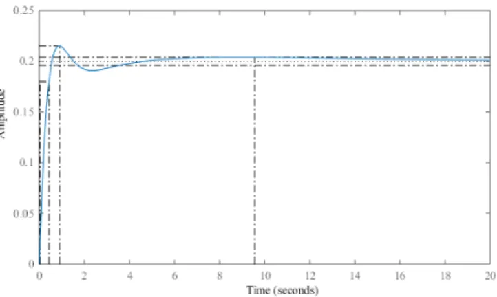
Example 2. The second example is the aircraft pitch con-trol problem from the Concon-trol Tutorials for Matlab and Simulink (Messner et al., 2017). The state-space model for one of Boeing’s commercial aircraft is given as:
˙ α ˙ q ˙ θ = "−0.313, 56.7, 0 −0.0139,−0.426,0 0, 56.7, 0 # "α q θ # + "0.232 0.0203 0 # δ, y= [0,0,1][α, q, θ]T (48)
Fig. 1. Step response for 0.2 radians
where α is the angle of attack, q is the pitch rate, θ is the pitch angle andδis the elevator deflection angle. The design requirements are the following: overshoot less than 10%, rise time less than 2 seconds, settling time less than 10 seconds, steady-state error less than 2%.
Using the LQR-based controller design approaches the controller parameter’s tuning is replaced by the tuning of the weighting parameters. This can relevantly reduce the time and complexity of the tuning process, mainly for large-scale multi-input multi-output applications. For more information and tuning approaches the readers are referred to books (Athans and Falb, 1966; Dorato et al., 2000) and references therein.
After a short iterative tuning all the requirements were fulfilled by Q = diag([0,0,0,0.6,28]), R = 1 and N = [0; 0; 0; 0;−4.5] (step response: Fig. 1) with rise time: 0.954 seconds, settling time: 9.5603 seconds, overshoot: 7.496%, steady-state error: 0%. The obtained realizable PID gains are: Kp = 5.1724, Ki = 1.7031, Kd = 3.0076, with filter
coefficientNf= 100.
Example 3. The third example is a simple uncertain MIMO system, which will be used to demonstrate the freedom in structurability what the oflqrcan give. For example, different controller types can be designed for each subsystem at once. The system with parametric uncer-tainty is given as:
G(s) = " h1,2i 10s+1, 2 s+1 1 s+1, h−3,−4i 10s+1 # , (49)
which can be transformed to the form (2) with matrices:
A1,2,3,4= −0.1, 0, 0, 0 0, −1, 0, 0 0, 0, −1, 0 0, 0, 0, −0.1 , B1= 0.1, 0 0, 2 1, 0 0, −0.3 , B2= 0.1, 0 0, 2 1, 0 0, −0.4 , B3= 0.2, 0 0, 2 1, 0 0, −0.3 , B4= 0.2, 0 0, 2 1, 0 0, −0.4 C1,2,3,4= h1,1,0,0 0,0,1,1 i , D1,2,3,4= h0,0 0,0 i .
Assume that we want to design a fully decentralized controller, more precisely a PI controller for the first subsystem and a PID for the second subsystem. In order to do so, let’s define the output matrix for the derivative part just for the second subsystem:Opt.Cdj=Cj(2,:). Finally, let us construct the structure matrixOpt.CS:
CS= h y1 y2 z1 z2 ydf2 u1 1, 0, 1, 0, 0 u2 0, 1, 0, 1, 1 i . (50)
Numerical solution has been carried out by SDPT3 (Toh et al., 1999) solver under OCTAVE 4.0 using YALMIP R20150918 (L¨ofberg, 2004). The obtained PI and PID gains by weighting matrices Q = In+li+ld, R = Im and N = 0n+li+ld×mare as follows: PI: Kp= 1.6344, Ki= 1.0014, PID:Kp=−1.2735, Ki =−0.5119, Kd=−0.0403. (51) 5. CONCLUSION
A new toolbox for Matlab and Octave is introduced in this paper. More precisely a function from the toolbox, which can be used to design a structurable robust LQR-based output feedback controller for uncertain LTI systems. The toolbox will soon be enriched by the discrete version of the presentedoflqrfunction. Moreover, the future plan is to include the author’s all recent results in linear parameter-varying (LPV)/ gain-scheduled output-feedback controller design as functions in the presented toolbox. For recent updates please visit: www.adrianilka.eu/oflqrtoolbox.htm
REFERENCES
Athans, M. and Falb, P. (1966).Optimal control. McGraw-Hill Publishing Company, Ltd, Maidenhead, Berksh, New York. Pp. 879.
Dorato, P., Abdallah, C.T., and Cerone, V. (2000).Linear Quadratic Control: An Introduction. Krieger Publishing Company.
Engwerda, J. and Weeren, A. (2008). A result on output feedback linear quadratic control. Automatica, 44(1), 265–271.
Ilka, A. and McKelvey, T. (2017). Robust discrete-time gain-scheduled guaranteed cost PSD controller design. In2017 21st Int. Conference on Process Control, 54–59. Ilka, A. and Vesel´y, V. (2017a). Robust LPV-based infinite horizon LQR design. In2017 21st International Conference on Process Control (PC), 86–91.
Ilka, A., Ottinger, I., Ludwig, T., T´arn´ık, M., Vesel´y, V., Miklovicov´a, E., and Murgaˇs, J. (2015). Robust Con-troller Design for T1DM Individualized Model: Gain-Scheduling Approach. International Review of Auto-matic Control (IREACO), 8(2), 155–162.
Ilka, A. and Vesel´y, V. (2014). Gain-Scheduled Controller Design: Variable Weighting Approach. Journal of Elec-trical Engineering, 65(2), 116–120.
Ilka, A. and Vesel´y, V. (2017b). Robust guaranteed cost output-feedback gain-scheduled controller design. IFAC-PapersOnLine, 50(1), 11355 – 11360. 20th IFAC World Congress.
Ilka, A., Vesel´y, V., and McKelvey, T. (2016). Robust Gain-Scheduled PSD Controller Design from Educa-tional Perspective. InPreprints of the 11th IFAC Sym-posium on Advances in Control Education, 354–359. Bratislava, Slovakia.
Kwakernaak, H. and Sivan, R. (1972). Linear optimal control systems. Wiley-Interscience.
L¨ofberg, J. (2004). YALMIP : A Toolbox for Modeling and Optimization in MATLAB. In Proceedings of the CACSD Conference. Taipei, Taiwan.
Messner, B., Tilbury, D., and JD, T. (2017). Control tutorials for matlab and simulink. Technical report, Creative Commons Attribution.
Molinari, B. (1977). The time-invariant linear-quadratic optimal control problem. Automatica, 13(4), 347 – 357. Mukhopadhyay, S. (1978). P.I.D. equivalent of optimal
regulatror. Electronics Letters, 14(25), 821–822. Rosenbrock, H. (1970). State-Space and Multivariable
Theory. Nelson, London, U.K.
Rosinov´a, D. and Vesel´y, V. (2004). Robust static output feedback for discrete-time systems - LMI approach. Periodica Polytechnica Ser. El. Eng., 48(3-4), 151–163. Rosinov´a, D. and Vesel´y, V. (2007). Robust PID decen-tralized controller design using LMI. Int. Journal of Computers, Communications & Control, 2(2), 195–204. Rosinov´a, D., Vesel´y, V., and Kuˇcera, V. (2003). A neces-sary and sufficient condition for static output feedback stabilizability of linear discrete-time systems. Kyber-netika, 39(4), 447–459.
Shamma, J.S. (2012). Control of Linear Parameter Vary-ing Systems with Applications, chapter An overview of LPV systems, 3–26. Springer.
Sturm, J. (1999). Using SeDuMi 1.02, a MATLAB toolbox for optimization over symmetric cones. Optimization Methods and Software, 11–12, 625–653.
Toh, K.C., Todd, M., and T¨ut¨unc¨u, R.H. (1999). SDPT3 – a MATLAB software package for semidefinite program-ming.Optimization methods and software, 11, 545–581. Trentelman, H.L. and Willems, J.C. (1991). The Dissipa-tion Inequality and the Algebraic Riccati EquaDissipa-tion, 197– 242. Springer Berlin Heidelberg, Berlin, Heidelberg. Vesel´y, V. (2001). Static output feedback controller design.
Kybernetica, 37(2), 205–221.
Vesel´y, V. (2005). Static output feedback robust controller design via LMI approach. Journal of Electrical Engi-neering, 56(1-2), 3–8.
Vesel´y, V. (2006). Robust controller design for linear polytopic systems. Kybernetika, 42(1), 95–110.
Vesel´y, V. and Ilka, A. (2013). Gain-scheduled PID cont-roller design. Jour. of Process Cont., 23(8), 1141–1148. Vesel´y, V. and Ilka, A. (2015a). Design of robust gain-scheduled PI controllers. Journal of the Franklin Insti-tute, 352(4), 1476 – 1494.
Vesel´y, V. and Ilka, A. (2015b). Unified Robust Gain-Scheduled and Switched Controller Design for Linear Continuous-Time Systems. International Review of Automatic Control (IREACO), 8(3), 251–259.
Vesel´y, V. and Ilka, A. (2017). Generalized robust gain-scheduled PID controller design for affine LPV systems with polytopic uncertainty. Systems & Control Letters, 105(2017), 6–13.
Vesel´y, V. and Rosinov´a, D. (2011). Robust PSD Con-troller Design. In M. Fikar and M. Kvasnica (eds.), Pro-ceedings of the 18th International Conference on Process Control, 565570. Tatransk´a Lomnica, Slovakia.
Vesel´y, V. and Rosinov´a, D. (2013). Robust PID-PSD Controller Design: BMI Approach. Asian Journal of Control, 15(2), 469–478.
Willems, J. (1971). Least squares stationary optimal con-trol and the algebraic riccati equation. IEEE Transac-tions on Automatic Control, 16(6), 621–634.
Zhou, K., Doyle, C.J., and Glover, K. (1996). Robust and optimal control. Prentice-Hall Inc., U.S. River, USA.